Climate Change, Land Use/Land Cover Change, and Population Growth as Drivers of Groundwater Depletion in the Central Valleys, Oaxaca, Mexico

Abstract

Groundwater depletion is an important problem driven by population growth, land use and land cover (LULC) change, climate change, and other factors. Groundwater depletion generates water stress and encourages unstainable resource use. The aim of this study is to determine how population growth, LULC change, and climate change relate to groundwater depletion in the Alto Atoyac sub-basin, Oaxaca, Mexico. Twenty-five years of dry season water table data from 1984 to 2009 are analyzed to examine annual groundwater depletion. Kriging is used to interpolate the region’s groundwater levels in a geographic information system (GIS) from mapped point measurements. An analysis of remotely sensed data revealed patterns of LULC change during a 34-year (1986–2018) period, using a supervised, machine-learning classification algorithm to calculate the changes in LULC. This analysis is shown to have an 85% accuracy. A global circulation model (GFDL-CM3) and the RCP4.5 and RCP8.5 scenarios were used to estimate the effects of climate change on the region’s groundwater. Estimates of evapotranspiration (using HELP3.5 code) and runoff (USDA-SCS-CN), were calculated. Since 1984, the region’s mean annual temperature has increased 1.79 °C and urban areas have increased at a rate of 2.3 km²/year. Population growth has increased water consumption by 97.93 × 10⁶ m³/year. The volume of groundwater is shrinking at a rate of 284.34 × 10⁶ m³/year, reflecting the extreme pressure on groundwater supply in the region. This research reveals the nature of the direct impacts that climate change, changing LULCs, and population growth have in the process of groundwater depletion.

1. Introduction

Groundwater is a complex component of any region’s hydrological system. Detailed information and descriptive data of the volumes, extent, and quality of groundwater supplies is usually very limited. What is known about the groundwater resources of a region is often sketchy and uncertain. Groundwater is storage of fresh water in aquifer systems which are subterranean layers of water-bearing permeable rock or unconsolidated materials. According to Arnell [1], the processes that control the recharge (R_e) ratios in aquifers are climate, topography, and the geological structure. Precipitation (P) provides the input into the aquifer system. Hydrological soil conditions control infiltration of water to the water table. However, the geological framework determines the capacity for water to flow at depths and can slow recharge rates. If the climatic and soil conditions generate R_e in excess of the capacity of the saturated matrix to transmit the R_e, then the permeability of the geological characteristics controls R_e rates [2]. The water balance (aquifer inflows and outflows) can be defined as the volume that is required to sustain groundwater use and groundwater-dependent ecosystem services for a region of interest, which could be delimited as an aquifer, a watershed, or a community [3]. Many social, economic, and environmental processes influence groundwater quantity and quality, and these systems are often difficult to predict. They therefore increase the complexity of groundwater management. Populations of every region of the world rely to some extent on groundwater. Due to its complexity, groundwater is a system that, once degraded, is very difficult to repair [4]. Groundwater is a vital source of fresh water for residential uses and for agriculture [5,6,7], and it plays a fundamental role in economic and food security [8]. Agriculture uses more freshwater than any other economic sector or activity. It accounts for about 70% of global freshwater withdrawals and 90% of freshwater consumption. Irrigation consumes 545 km³ of groundwater per year. Groundwater provides 43% of water consumed (1277 km³) for irrigation ever year [5].

Water scarcity is a widespread and challenging problem in Mexico, regularly presenting moderate and severe scarcity from February to May or June [9]. The problem has worsened dramatically over the last three decades. In the Central Valleys of Oaxaca, two forces are the main drivers of increasing groundwater demand: agriculture, the main economic activity using groundwater (more than 80% of groundwater is used for agriculture), and population, which has increased by about 76% since the 1980s. Agriculture in Oaxaca has experienced abandonment due to poverty, and rural-to-urban migration has increased the pressure of urban water demand on rural groundwater supplies. Changing consumption habits and low-tech irrigation infrastructure have also intensified the pressures on groundwater. Climate change (CC) is now an additional stress. In combination with population growth and redistribution, and land-use and land-cover (LULC) changes, shifts in weather patterns and increasingly unanticipated shifts in components of climate magnify stresses on freshwater supplies [10,11,12,13,14,15]. The pressures are so great that some parts of the Central Valleys of Oaxaca are experiencing significant pollution problems due to overexploitation, poor waste management infrastructure, and shrinking aquifers.

New tools and techniques are needed to extract and analyze data to evaluate present and future groundwater conditions. Probabilistic tools to determine the sensitivity and uncertainty of the analytical innovations can provide some insight. LULC changes can be used to assess the trends in groundwater supplies. Remote sensing can be used to determine where those changes are greatest in order to fill in data gaps. Water table monitoring at wells provides instantaneous assessments of the effects of R_e and extraction. Water table point data must be spatially extrapolated to visualize regional change. Therefore, geostatistical methods are vital for data analysis. The distribution and quality of field data dictates the best methods to use. Kriging, for example, is an interpolation method that has been used in many groundwater studies [16,17,18,19,20,21]. Kriging can be applied to a small and sparsely distributed observation sample and yields error estimates to characterize the accuracy of its output.

Assessing the hydrological effects of climate change, LULC, and population growth is of vital importance for land use planning and water resource management. Especially because groundwater supports drinking water for the population and irrigation for agriculture in the Central Valleys of Oaxaca. This research combines empirical data from a network of wells, remotely sensed data, groundwater models, and a geographic information system (GIS) for data management and analyses of historical patterns of groundwater uses, demands, and supplies in the Central Valleys of Oaxaca in order to spatially predict the future demands and supplies in the contexts of anticipated growth and change of population, land use and land cover (LULC), and climate. The results can help pinpoint areas that may (or may not) contribute sufficient R_e to meet the future demands for groundwater in the region. Such knowledge can aid planning for engineered R_e infrastructure for selected zones and the use of irrigation management strategies with effective water-consumption policies that achieve water supply goals.

Study Area

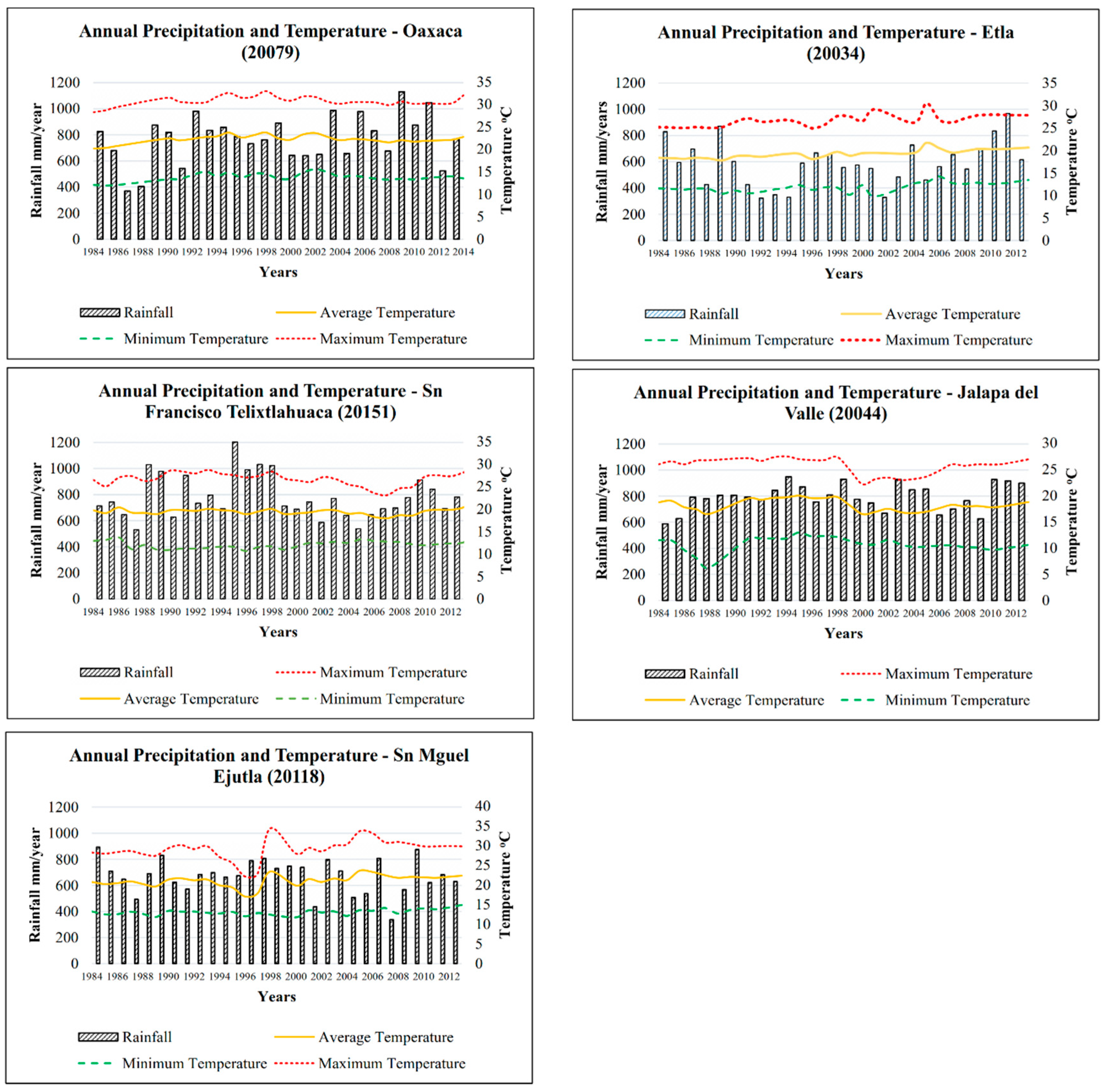
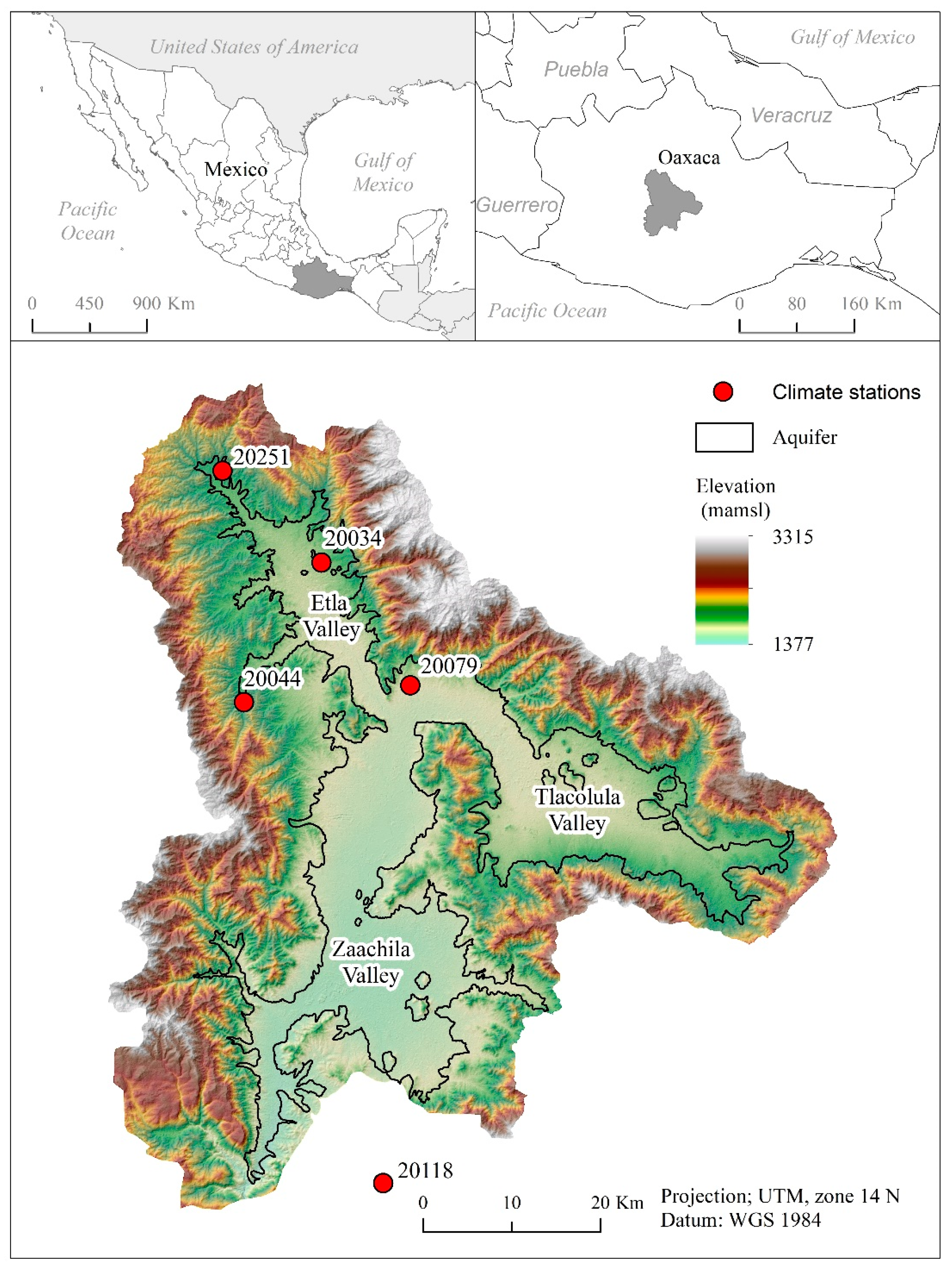
The study area is a basin located between 16°30′ and 17°25′N and 96°15′ and 97°00′W. Three valleys in the basin, the Etla, the Tlacolula, and the Zaachila (from Zimatlán to Ocotlán), are collectively referred to as the Central Valleys of Oaxaca (Figure 1). The Central Valleys border the Mixteca region to the west, the Cañada region to the northwest, the Sierra de Juárez to the north, the Tehuantepec Isthmus region to the east, and the Sierra Madre del Sur to the south. The Alto Atoyac sub-basin has a surface area of 3744.64 km², with an approximate aquifer surface of 1130 km², the annual R_e ranges from 153.6 to 169 million m³ [22], with an average annual P (P) of 741 mm/year and annual average temperature (T) of 19.96 °C. The region’s bedrock includes metamorphic gneiss and schists, limestones, and rhyolites. The metamorphic rocks and extrusive volcanic rocks constitute the impermeable borders of the sub-basin [22] (for more detail of the geology see [23] and [24]. The 396 km long Atoyac River is the main river course through the Central Valleys.

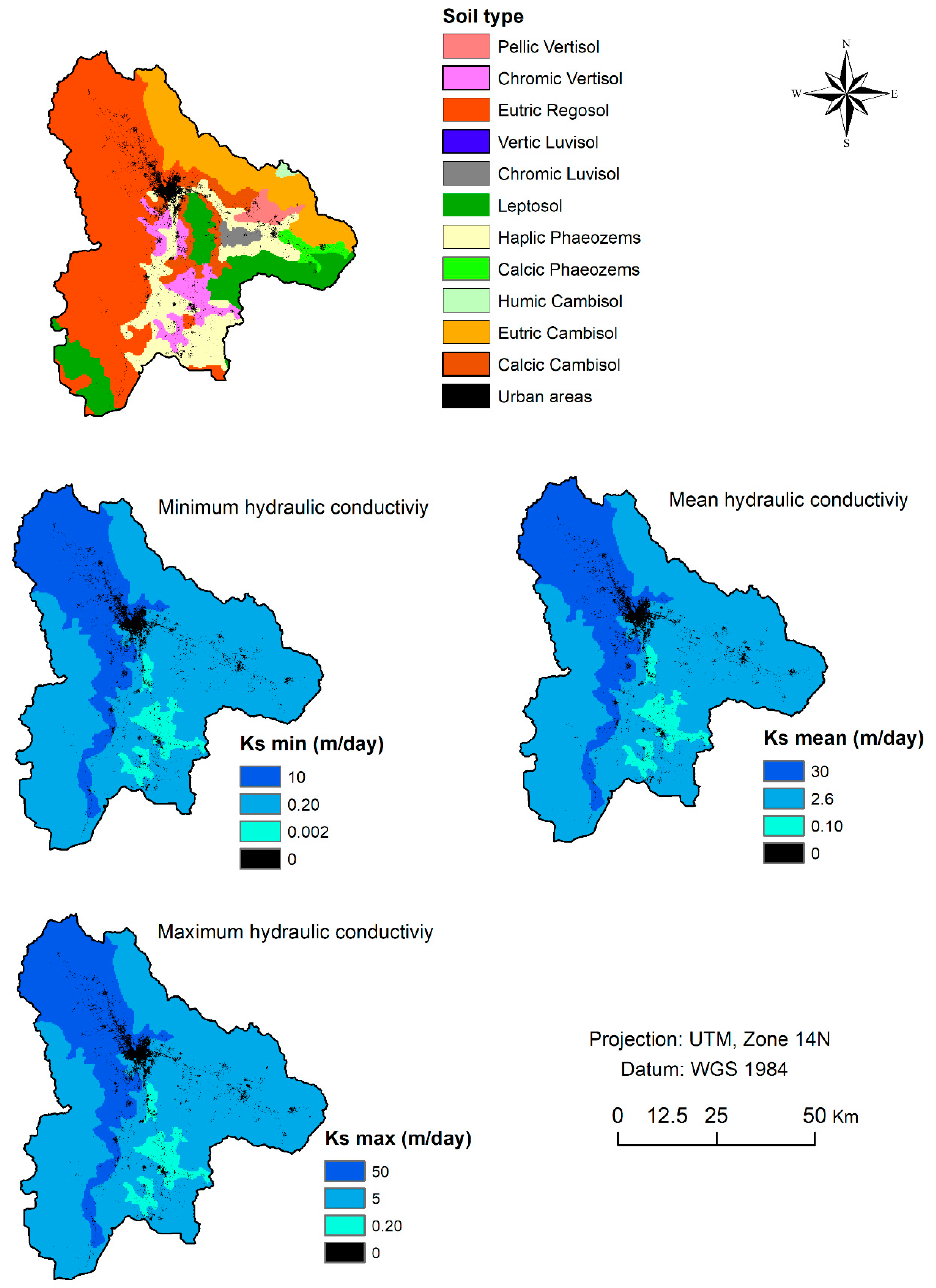
Agriculture is the main economic activity of the rural portions of the sub-basin, particularly in the Zaachila and Etla Valleys, the two largest agricultural districts. Agriculture is estimated to use 87.6% of the groundwater of the study area [22]. The aquifer of the Central Valleys is unconfined and is composed of alluvium, a heterogeneous mixture of unconsolidated sediments. Its thickness ranges from 15 m to 100 m, thinning toward the basin’s edges. The region’s water table is shallow (0.2 m to 20 m) and there are areas of high permeability (Figure 2). Intensive agriculture in the region has increased the likelihood of overexploitation. A large depletion cone has been identified in the Zaachila Valley.

2. Materials and Methods

2.1. Meteorological Stations

Climatological data are limited for the area. Five meteorological stations with time-series records of more than 30 years were selected (Figure 3). The climatic information was obtained from Mexico’s CLICOM (Climatological Computing) project, Servicio Meteorológico Nacional (National Meteorological Service) through CICESE (available at http://clicom-mex.cicese.mx/) for the period from 1984 to 2012 and the year 2014, to analyze the evolution of P and T (

Table 1. Statistic values of the meteorological stations.

Meteorological Station	Mean				STD
	Tmin (°C)	Tmean (°C)	Tmax (°C)	P (mm/year)	Tmin (°C)	Tmean (°C)	Tmax (°C)	P (mm/year)
20034	11.81	19.24	26.66	589.53	1.04	0.95	1.36	169.67
20079	13.75	22.23	30.71	768.70	0.90	0.91	1.08	188.25
20118	13.10	21.08	29.06	672.18	0.75	1.48	2.60	129.72
20151	12.11	19.42	26.73	780.48	0.89	0.75	1.50	164.69
20044	10.75	18.19	25.62	793.72	1.38	1.11	1.57	101.22

).

2.2. Climate-Change Scenarios

Two scenarios of CC based on the projections produced by RCP4.5 and RCP8.5 are used to assess the impacts of changing climate on groundwater volumes. The first is a scenario based on stabilizing future climates without thermal overshoot. Total radiative forcing (4.5 W/m²) is stabilized after 2100. RCP4.5 includes long-term, global emissions of short-lived species of greenhouse gases and LULC in a global economic framework. This scenario was developed by the Global Change Assessment Model (GCAM) modeling team at the Pacific Northwest National Laboratory’s Joint Global Change Research Institute (JGCRI) [25,26]. The second scenario, RCP8.5, assumes high population growth and relatively slow income growth with modest rates of technological change and energy intensity improvements, leading to long-term high energy demand and unrestricted GHG emissions in the absence of global-warming mitigation policies [27].

A global circulation model (GCM), GFDL-CM3, was chosen from the last update of the Climate Change Scenarios for Vulnerability and Adaptation Impact studies conducted for Mexico and Central America [28]. These scenarios have a high spatial resolution of 30″ × 30″. Two scenarios were analyzed for RCP4.5 and RCP8.5 conditions in three time-horizons: near (2015–2039), medium (2045–2069) and far (2075–2099) (Figure 4a,b, Figure 5a,b).

2.3. Calculating Evapotranspiration (ET)

To estimate future groundwater supplies, the balance of the values of the components of the hydrological system, like ET rates, must be calculated for given future T and P scenarios. The HELP model, used for predicting landfill hydrologic processes, can also be used to estimate water-balance parameters, requiring the following inputs: (1) weather (P, solar radiation, T, and ET); (2) soil (porosity, field capacity, wilting point, and hydraulic conductivity), and (3) engineering design data (liners, leachate and runoff collection systems, and surface slope) [29,30].

To calculate ET, the input parameters included in the HELP model were evaporative depth zone, maximum leaf area index, starting and ending dates of growing season, average wind speed, and quarterly relative humidity [30]. A depth of 100 cm was used as the maximum depth at which water can be removed by ET, which corresponds to the average plant root length in the area. ET was calculated for the historical climate data and for the data produced by the RCP4.5 and RCP8.5 climate scenarios for the 2015–2039, 2045–2069, and 2075–2099 horizons.

2.4. LULC Change and Runoff ($R_u$)

2.4.1. Satellite Imagery Acquisition and Preprocessing

Landsat imagery was used to discern LULC change and to calculate its effects on groundwater supplies over the last three decades as these data span the period of interest. Five temporally equidistant dates were chosen based on data availability, data quality (minimization of cloud coverage), and season (dry season) (

Table 2. Satellite imagery used for the remote sensing analysis.

Satellite	Sensor	Date
Landsat 5	TM	20 January 1986
Landsat 5	TM	26 January 1994
Landsat 7	ETM+	13 March 2002
Landsat 5	TM	22 January 2010
Landsat 8	OLI	1 March 2018

). To encompass the study area, two Landsat scenes for each date (024048 and 024049) were acquired. All images have the same spatial resolution (30 m), but data were sensed by distinct satellites and sensors at different times of the year. Therefore, each scene was radiometrically corrected by converting the raw digital numbers (DNs) into top of atmosphere (TOA) reflectance values to enable interannual comparisons. After mosaicking the Landsat scenes by date, the resulting five images were clipped to the study area. The 1986 image was slightly masked by clouds and cloud shadows along the northeastern border. Though only 0.26% of the pixels were affected, they were removed from the analysis to avoid misclassification.

2.4.2. Classification and Change Detection

According to the LULC characteristics of the study area and based on the spatial resolution of the images, five classes of LULC were assigned: urban, agriculture, grassland, forest, and water. Following this scheme, samples of each class were collected using visible, near infrared, and short-wave infrared spectral bands, as well as a digital elevation model (DEM) as ancillary data. The samples were used to train a random-forest classifier [31]. This supervised machine-learning classification algorithm is nonparametric and overcomes the issue of individual decision trees overfitting to the training sample data. To determine classification accuracy, reference points were compared to the classification results at the specific locations. The calculation of the sample size for reference points was based on binomial probability theory with an expected accuracy of 85% and allowable error of 5% [32]. Thus, 204 randomly distributed reference points were classified by visual interpretation of finer resolution imagery available on Google Earth. After classifying and assessing the accuracy of the five images, post-classification comparison techniques were used to detect LULC change. Image pairs of subsequent dates were compared by cross-tabulation of the LULC statistics. The resulting four change-detection matrices (1986–1994, 1994–2002, 2002–2010, 2010–2018) reflect conversion of specific LULC types to other classes. The total area assigned to each class at each time node was also calculated to evaluate the changes over the entire 32-year period. The forest class was arbitrarily attributed to all cloud-affected pixels to facilitate a pixel-based comparison to the 1986 image, the only scene affected by clouds. This was justified by the fact that all cloud-covered pixels were surrounded by forest and they remained unchanged over the study period.

2.4.3. R_u Rates by LULC Class

LULC change impacts local water dynamics, either by changing groundwater R_e patterns or runoff due to increased impervious surfaces through urbanization or slowing runoff with revegetation of the surface. Assessing the direct impact of land cover change allows extrapolation to the study region’s hydrology. The runoff was calculated with the Soil Conservation Service (SCS) curve number (CN) method which is described in detail in SCS [33]. The curve-number method was used for four reasons: (1) it is widely accepted; (2) it is computationally efficient; (3) the required input is generally available, and (4) it can conveniently handle a variety of soil types, LULCs, and management practices [29]. The runoff equation to be evaluated is:

$$R_u=\frac{{\left(P-0.2\ast S\right)}^2}{\left(P+0.8\ast S\right)}$$

(1)

where R_u is runoff (inches), P is precipitation (inches), and S is potential maximum retention after $R_u$ begins (inches). S is related to the soil and cover conditions of the watershed through the CN. CN has a range of 0 to 100; 0 indicates conditions of high permeability and 100 indicates complete impermeability. S can be calculated as:

$$S=\frac{1000}{CN}-10$$

(2)

There are seven different soil types in the study area, and they can be grouped into two soil types according to their hydrological features (hydraulic conductivity) (Figure 2). The curve number was calculated for the four LULCs in combination with the two soil types.

Urban growth was projected as a linear trend for the study area. It was assumed that agricultural areas would continue to be transformed to urban LULCs, as our change analysis of the Landsat scenes showed. By comparison, the other land cover classes were unaltered. $R_u$ amounts were calculated based on the variations of P under both of the climate-change scenarios and over the three time horizons.

2.5. Water Balance

Water balance was calculated from annual P, ET, and $R_u$ to assess the impacts of various changes on water recharge. P was the only input to the system and $R_u$, ET, were the outputs to obtain R_e.

2.6. Sensitivity Analysis for the Water Balance

Sensitivity analysis evaluates the impact of changes in a model’s parameters, inputs, or (initial) states on the model’s output variable of interest [34]. A Monte Carlo method was used to determine the sensitivity of the water balance parameters. This is a stochastic technique based on the use of random numbers and statistics to evaluate the consequences of altered inputs. Multiple evaluations of the model were performed with probabilistically selected model inputs to evaluate and quantify the uncertainty in the predictions of the model, and to identify the input factors that gave rise to the uncertainty [35,36]

Monte Carlo simulations were executed using the software SimLab V2.2 (Simulation Environment for Sensitivity and Uncertainty Analysis) downloaded at https://ec.europa.eu/jrc/en/samo/simlab. It consists of three modules: the statistical preprocessor module, the model specification and execution module, and the statistical postprocessor module. To use SimLab, the user performs the following operations [35]:

• Select a range and distribution for each input factor.
• Generate a sample of elements from the distribution of the inputs previously specified.
• Feed the model with the sample elements and produce a set of outputs.
• Use the results of the model outputs for uncertainty analysis.

The input variables for the model were P, mean annual T, LULC (urban, agriculture, grassland, and forestland), and the results of modeled calculations for the five meteorological stations (ET, $R_u$, and recharge). Randomly sampled values were taken to reflect the cardinality of the model’s inputs and output.

2.7. Partial Correlation Coefficient (PCC)

Correlation between variables are indicated by partial correlation coefficients. These coefficients are guided by the principles of correlation and partial correlation; however, when relationships between input factors are nonlinear, the correlation coefficient could be low. To solve the problem of nonlinear data, a rank transformation was used. In this process the data are replaced with their corresponding ranks (from 1 for smallest to N for the largest observation) [35].

Variation of rank of partial correlation coefficients are −1 to +1. A value close to the upper or lower limits shows a strong influence of the input factors over the output values. Usually, PRCC values >+0.5 or <−0.5 are considered significant. Positive or negative values indicate the nature of the relationship (direct or inverse) between the input and output variables [36]

2.8. Water Table Change and Calculation of Volume Storage Change

The water table depth was measured as piezometric head (in m) for five years: 1984, 2001, 2003, 2007, and 2009 (Figure 6). A geostatistical interpolation technique was used to represent the distributed depth to water table throughout the study area. This technique allowed for scenario-based prediction surfaces that have measurable levels of accuracy [37]. This well-known technique, kriging, denotes interpolators stochastically. Kriging statistically predicts values using an unbiased linear estimator. It is often the best method for interpolation because it factors in the number and spatial configuration of observation points, the positions of the data points within the region of interest, the distances between the data points with respect to the area of interest, and the spatial continuity of the interpolated variable [17]. It also generates an estimate of the error of its calculations.

The changes in depth to water table can be used to calculate the change in volume of the aquifer from one time period to the next. To calculate the change of volume for each period, a triangular irregular network (TIN) model was constructed in GIS to calculate the volume for each of the four intervening periods between the estimates: 1984–2001, 2001–2003, 2003–2007 and 2007–2009 (Figure 7). The piezometric surface for 1984 was used as the baseline.

2.9. Population Growth and Water Consumption

According to the Instituto Nacional de Estadística Geografía e Informática (INEGI—the National Institute of Geographic Statistics and Information), the population of the Central Valleys of Oaxaca has grown at a rate of 2.32% per year from 1980 to 2010 [38,39]. Population growth trends since 1980 were projected to 2039, 2045, 2069, 2075, and 2099 to estimate future water needs. Projected needs translate to groundwater extraction and must be set into the context of CC to determine the predicted impacts on future supplies. Historically, water consumption in the study area ranged from 48 to 384 liters per person per day (LPD) [40]. The average of 216 LPD was used as a constant on which future consumption projections could be made.

3. Results

3.1. Climatology, Cclimate-Change Scenarios and ET

Five meteorological stations provided P and T records for the Central Valleys. Water resources are dynamic yet examining meteorological data climatologically can enable examination of the changing patterns of water supplies in a region. Over the last 30 years, empirical measurements indicate that there have been changes in annual P amounts. Empirical data reveals an increase in annual T_mean in the Central Valleys. Annual T_mean has increased by 1.76 °C over the past 30 years, while the annual T_min and T_max have increased 1.109 °C and 2.4 °C, respectively (

Table 3. Changes in Annual T_mean from 1984 to 2014.

Meteorological Station	Tmin (°C)	Tmean (°C)	Tmax (°C)
20034	1.877	2.297	2.662
20079	1.439	2.560	3.681
20118	1.668	1.597	1.531
20151	1.414	2.286	3.158
20044	−0.854	0.058	0.970
Average	1.109	1.760	2.400

).

The RCP4.5 projects P will increase in the near term and medium term (2015–2039 and 2045–2069) of 23.03 mm/year and 26.56 mm/year, respectively. In the long term (2075–2099), P will diminish at a rate of 15.58 mm/year compared to the contemporary average. The RCP8.5 scenario projects that the annual average P will diminish by 3.58, 20.59, and 19.04 mm/year in the near, medium, and distant periods (

Table 4. Projections of P based on RCP4.5 and RCP8.5 scenarios using the GFDL-CM3 global circulation model.

Scenario	P (mm/year) 2015–2039	P (mm/year) 2045–2069	P (mm/year) 2075–2099
RCP4.5	751.34	754.87	712.73
RCP8.5	724.73	707.72	709.27
Historical *	728.31

* 1984–2014.

).

The CC scenarios indicate that annual T_mean and average T_max will increase each year. Rising global T_mean of up to 2 °C followed by stabilization and of 4 °C indicate that water scarcity will increase exponentially as a product of warming in many parts of the world [41] (

Table 5. Projected changes of annual T_mean, T_min, and T_max under the RCP4.5 and RCP8.5 scenarios.

Scenario	Tmean (°C) 2015–2039	Tmean (°C) 2045–2069	Tmean (°C) 2075–2099	Tmin (°C) 2015–2039	Tmin (°C) 2045–2069	Tmin (°C) 2075–2099	Tmax (°C) 2015–2039	Tmax (°C) 2045–2069	Tmax (°C) 2075–2099
RCP4.5	19.49	20.52	21.05	12.04	13.07	13.39	26.97	28.16	28.82
RCP8.5	19.52	21.24	22.98	12.16	13.83	15.60	26.92	28.72	30.41
Historical *	18.03			10.71			25.36

* 1984–2014.

). In the first climate scenario (RCP4.5) T_mean will increase by 1.46, 2.49, and 3.02 °C, and in the second (RCP8.5) the increases will be 1.49, 3.21, and 4.95 °C for 2015–2039, 2045–2069 and 2075–2099, respectively.

ET rates are calculated using annual P and T_mean. ET projections under both scenarios show a trend that is increasing from historical rates (

Table 6. Historical and projected ET rates under both scenarios and the percentages of increase from the present.

Evapotranspiration (mm/year)
	2015–2039	%Increase	2045–2069	%Increase	2075–2099	%Increase
RCP4.5	472.673	3.895	484.088	6.405	468.128	2.896
RCP8.5	460.920	1.312	467.018	2.652	479.798	5.462
Historical *	454.95

* Calculated as the annual average of all meteorological stations for the period of study.

). However, under RCP4.5, the trend peaks in the medium-term future and diminishes as T_mean diminishes after overshoot. Under RCP8.5, increasing rates of ET continue into the distant future. The increase of 1.46 °C above the current annual T_mean (scenario RCP4.5 in Table 4) for the near term translates to a rate of increase of 3.9% above the present rate of ET. An increase of 2.49 °C for the medium time horizon (scenario RCP4.5) yields an expected increase of 6.49% above the contemporary rate of ET.

3.2. LULC Change and $R_u$

LULC change affects the water balance by changing $R_u$ and infiltration and contributes to water supply problems. Another connection to water scarcity is the linkage of LULC and activities to water demand. For example, the growth and intensification of agriculture increases water extraction [42]. Industrial development tends to demand more water than does residential development, but lifestyles and culture (private swimming pools, lawns, golf courses, for instance) certainly distinguish water-heavy LULCs from water-light LULCs.

Historical LULC change in the Central Valleys has been dramatic over the thirty-year study period. From 1986 to 2018, urban land has increased from 0.85% of the sub-basin surface to 2.86% of the area (

Table 7. LULC in the Alto Atoyac sub-basin for five years.

Class	Area (km2)
	1986	1994	2002	2010	2018
Urban	33.16	48.94	63.82	94.95	111.65
Agriculture	1227.45	1238.67	1246.24	1183.29	1183.93
Grassland	763.78	749.62	689.18	694.60	728.37
Forest	1882.57	1870.63	1909.67	1930.65	1884.69
Water	3.42	2.52	1.47	6.89	1.74
Total	3910.37	3910.37	3910.37	3910.37	3910.37

). Agricultural land has decreased slightly from 31.39% to 30.28%. Forestland increased slightly from 48.14% to 48.2%. Grassland diminished from 19.53% to 18.63%. Surface water decreased from 0.09% to 0.04%. The trend of the agricultural decline, however, has been neither constant nor consistent. Between 1986 and 1994, agricultural land increased by 11.2 km² and from 1994 to 2002 it grew another 7.57 km². However, from 2002 to 2010, farmlands decreased by 62.95 km², and from 2010 to 2018, 0.64 km² were converted to agriculture. Similarly, forested lands had gained 60.02 km² between 1994 to 2010; however, after 2010, 45.96 km² were changed to other uses.

A trend line for urban LULC follows a direct linear relationship in the study region and can be approximated with the equation:

$$U=2.5374\ast Y-5009.3 R^2=0.9823$$

(3)

where U is the area of urban LULC in km² and Y is the period (in years) of projected increase to be calculated.

The other LULC classes don’t exhibit a linear trend. Changes in the other LULC categories over the last 32 years have been relatively minor. For example, forestland was nearly stable from 1986 to 2018. Forest cover increased by only 2.12 km². Agriculture covers less land in 2018 than it did in 1984, as 43.52 km² were lost to urbanization. The result is that because urban LULC increased, $R_u$ has increased from urban land by 7.58 mm/year (

Table 8. $R_u$ values for the historical climate normal and for the five LULC categories.

${\mathit{R}}_{\mathit{u}}$ (mm/year) for the Historical Climate Normal
LULC	1986	1994	2002	2010	2018
Urban	3.21	4.73	6.17	9.18	10.79
Agriculture	104.07	105.02	105.66	100.32	100.38
Grassland	49.20	48.29	44.39	44.74	46.92
Forest	64.76	64.34	65.69	66.41	64.83
Water	0.00	0.00	0.00	0.00	0.00
Total $R_u$	221.23	222.38	221.91	220.65	222.92

). Even though $R_u$ from urban areas is greatest and though there has been an increase of urban LULC, it seems to not have had much of an impact in total $R_u$ since 1986. Agriculture accounts for 45.03% of all runoff. Urban LULC is only a small portion (2.89%) of the sub-basin.

values for the historical climate normal and for the five LULC categories

Projecting changes in $R_u$ due to projected LULC change and changing climates using the two scenarios reveals that by the end of the century, urban $R_u$ may nearly double during the period 2018 to 2099 (

Table 9. $R_u$ values for the climate-change scenarios by LULC.

$R_u$(mm/year) in the RCP4.5 Climate-Change Scenario
LULC	2039	2045	2069	2075	2099
Urban	16.40	18.00	24.10	24.20	29.96
Agriculture	98.93	98.06	92.71	86.27	81.22
Grassland	48.40	48.63	48.63	45.91	45.91
Forest	66.88	67.19	67.19	63.44	63.44
Water	0.00	0.00	0.00	0.00	0.00
Total $R_u$	230.61	231.88	232.63	219.82	220.53
$R_u$(mm/year) in the RCP8.5 Climate-Change Scenario
LULC	2039	2045	2069	2075	2099
Urban	15.82	16.88	22.60	24.08	29.81
Agriculture	95.43	91.94	86.92	85.85	80.82
Grassland	46.69	45.59	45.59	45.69	45.69
Forest	64.51	63.00	63.00	63.13	63.13
Water	0.00	0.00	0.00	0.00	0.00
Total $R_u$	222.44	217.40	218.10	218.76	219.46

). This is projected to happen despite decreasing P. By contrast, $R_u$ for the other LULCs should diminish over the 81-year projection in both the RCP4.5 and RCP8.5 scenarios, largely because of diminishing P. Thus, due to urbanization of rural (particularly agricultural) lands, water supply will be diminished at a rate that is greater than is the effect of CC.

3.3. Water Balance

The potential for R_e has been changing since 1986 (

Table 10. Water balance in Alto Atoyac sub-basin from the climate record.

Water Balance	1986	1994	2002	2010	2013
Mean Annual P * (mm/year)	629.42	666.36	583.23	935.62	794.80
ET (mm/year)	405.98	434.07	391.15	405.98	498.45
Runoff (mm/year)	221.23	222.38	221.91	220.65	221.5
Potential Re (mm/year)	2.21	9.91	−29.83	308.99	74.5

* From the all five meteorological stations.

). This has been due to the interactions between increasing annual T_mean, rainfall variations and urbanization in the study region. R_e potential has increased by 72.29 mm/year.

There appear to be reductions of groundwater R_e by 2039 (26.44 mm, 35.48%) under the RCP4.5 scenario compared to the 2013 rate. However, there would be a reduction of 44.47% by 2039 under the RCP8.5 scenario (

Table 11. Water balance for RCP4.5 and RCP8.5 CC scenarios.

RCP4.5 CC Scenario
Water Balance	2039	2045	2069	2075	2099
Mean Annual P (mm/year)	751.34	754.87	754.87	712.73	712.73
ET (mm/year)	472.67	484.09	484.09	468.13	468.13
$R_u$ (mm/year)	230.61	231.88	232.63	219.82	220.53
Potential Re (mm/year)	48.06	38.90	38.15	24.78	24.07
RCP8.5 CC Scenario
Water Balance	2039	2045	2069	2075	2099
Mean Annual P (mm/year)	724.73	707.72	707.72	709.27	709.27
ET (mm/year)	460.92	467.02	467.02	479.8	479.8
$R_u$ (mm/year)	222.44	217.40	218.10	218.76	219.46
Potential Re (mm/year)	41.37	23.30	22.60	10.71	10.01

). At the most distant horizons of both scenarios, potential R_e is projected to decrease 67.69% (RCP4.5) and 86.56% (RCP8.5), indicating that there would be groundwater availability problems in the future.

3.4. Sensitivity Analysis

Sensitivity indices represent the sensitivities of RU, ET, and Re values to changes in P, T_mean, and changes in urban, agricultural land, grassland, and forestland proportions. Probability distribution of the input factors have to be chosen (

Table 12. Probability distribution and range of values.

Input Factors	Probability Distribution	Range	Most Probable Number (MPN)
Rainfall	Triangular	[200, 1300 mm/year]	568
Temperature	Triangular	[5, 35 °C]	15
Urban	Uniform	[0, 3910.38 km2]	600
Agriculture	Uniform	[0, 3910.38 km2]	490
Grassland	Uniform	[0, 3910.38 km2]	1792
Forest	Uniform	[0, 3910.38 km2]	3724

), and the correlation among the parameters have to be calculated (

Table 13. Correlation matrix for the input parameters.

	Rainfall	Tmean	Urban	Agriculture	Grassland	Forest
Rainfall	1	−0.0395	0.119	−0.101	−0.074	0.020
Tmean		1	0.201	−0.114	−0.138	0.132
Urban			1	−0.709	−0.860	0.879
Agriculture				1	0.394	−0.707
Grassland					1	−0.819
Forest						1

). A total of 10,000 random values were generated to determine the implications of the LULC assuming significant changes of the values which varied from 0 to 3910.38 km² with uniform distributions and the changes in Rainfall and Temperature with a triangular distribution.

The sensitivity index of Ru is positive (direct) for P, urban, and agriculture, which indicates that increases in these variables leads to increases in Ru. In contrast, the sensitivity index of R_e is negative (inverse) with respect to T_mean, urban, and agricultural areas. (

Table 14. Partial rank correlation coefficient and ranks for the input factors.

	Sensitivity Indices
	${\mathit{R}}_{\mathit{u}}$		ET		Re
Input factors	PRCC	Rank	PRCC	Rank	PRCC	Rank
P	0.986	1	0.920	1	0.784	2
Tmean	−0.010	6	0.789	2	−0.868	1
Urban	0.761	2	0.011	3	−0.523	3
Agriculture	0.614	5	0.007	5	−0.367	6
Grassland	−0.644	4	0.017	4	0.410	5
Forest	−0.678	3	0.005	6	0.457	4

and Figure 8).

P is the most sensitive output variable to input factors with its indices significantly larger than +0.5 and reaching the highest value of 0.98 and 0.92 for R_u and ET. T_mean is sensitive to ET with and index of 0.798 and for Re with and index of −0.864, representing an inverse relationship. Urban, agriculture, grassland, and forest are significant in the increase and decrease of $R_u$ with and index higher than 0.5. T_mean, Urban, Forest areas seem to cause significant changes in R_e with indices of −0.86, −0.52, 0.457, but they show an inverse relationship (T_mean, urban), indicating that increases in these inputs could reduce R_e.

If sensitivity analysis is conducted with the empirical values measured at the five meteorological stations, a total of 139 inputs are generated. The model based on empirical data is not sensitive to changing forest area because it has not changed much in the study area. The analysis will evaluate only the empirical contribution of forestland to the region’s runoff. It will not evaluate extreme reductions of any of the LULC categories. Forest area represented 48.2% of the total area and accounts for 21.04% of the total runoff (in 2018). The area of change in forest area has been very small—a STD of 24.18 km² and average coverage of 1895 km². This forest dynamic is probably due to conservation efforts in the region, the ejido and communal land ownership regimes, the indigenous tenants, and decreased farming and less cultivation. In Oaxaca, this is evident by a resurgence of forests [43,44]. Similar results to Minnig et al. [45] can be found, indicating that urban increases and forest decrease can decrease ET and increases the likelihood of R_e, but these results are not significant with PRCC values of −0.122 and 0.002, respectively.

Accuracy in input factors is important in estimation of R_u, R_e, and ET, but the results of the MC sensitivity analysis reveal that accuracy of measurements particularly with P, T, and urban and forest areas is critical. Indicating the CC and human impacts in the area will affect the area in the future.

3.5. The Impacts of Population Growth on Groundwater

Population growth has contributed to raising rates of groundwater extraction by increasing consumption for different uses. CC is projected to decrease R_e due to climate change [22]. The region’s population growth rate has been 2.32% annually. The population nearly doubled between 1984 and 2010, from 603,009 to 1,033,884 (

Table 15. Water consumption in the Alto Atoyac sub-basin.

Year	Population	Water Consumption 48 LPD (Mm3)	Water Consumption 216 LPD (Mm3)	Water Consumption 384 LPD (Mm3)
1984	603,009	10.56	47.54	84.52
1986	649,293	11.38	51.19	91.00
1990	718,942	12.60	56.68	100.77
1994	773,122	13.55	60.95	108.36
2001	877,946	15.38	69.22	123.05
2003	910,426	15.95	71.78	127.61
2007	979,037	17.15	77.19	137.22
2009	1,015,257	17.79	80.04	142.30
2010	1,033,884	18.11	81.51	144.91
2018	1,242,099	21.76	97.93	174.09
2039	2,010,607	35.23	158.52	281.81
2045	2,307,227	40.42	181.90	323.38
2069	4,000,766	70.09	315.42	560.75
2075	4,590,990	80.43	361.95	643.47
2099	7,960,844	139.47	627.63	1115.79

LPD: Liters per person per day, Mm³: Millions of cubic meters.

). This growth increased consumption by 50.39 Mm³ (from 47.54 Mm³ in 1984 to 97.93 Mm³ in 2018 (average water consumption rate of 216 LPD), which is nearly a two-fold growth (94.33%) over 34 years. This trend, if it continued unabated, is not sustainable.

The connection between water consumption and urbanization is apparent when one plots water consumption rates against the changing areal extent of urban LULCs (Figure 9). The direct linear relationship demonstrates the greater pressure that per unit area urban LULCs and the systems of cities put on water resources.

3.6. Groundwater Volume Storage Change

A water table evaluation allows us to examine the evolution of groundwater extraction rates through the period of record (

Table 16. Extracted volume in different periods (volume storage change).

Period	Volume Storage Change in the Period (m3)	Annual Average Change (m3)	Annual Average Human Consumption (m3)	Agriculture/other Uses (m3)	Annual Average Recharge (m3)
1984–2001	1964 × 106	115.53 × 106	47.54–69.22 × 106	57.15 × 106	138.910–158.77 × 106
2001–2003	695.1 × 106	347.5 × 106	69.22–71.78 × 106	277 × 106	158.77–160.491 × 106
2003–2007	1370 × 106	342.5 × 106	71.78–77.19 × 106	325.95 × 106	160.491–170.89 × 106
2007–2009	663.6 × 106	331.8 × 106	77.19–80.04 × 106	253.185 × 106	170.89–171.75 × 106

. Groundwater extraction is closely related to the intrinsic and extrinsic conditions of the sub-basin, the anthropogenic effects on weather conditions, the increasing area of impervious surfaces, agriculture water demand, and population growth. Together, they can accelerate the rate of groundwater extraction.

Our analysis of the spatial and temporal nature of the water table in the Alto Atoyac sub-basin from 1984 to 2009 reveals growing groundwater depletion, especially in zones of agricultural activities. The areas of the aquifer with the most decline are the areas that have the greatest need for water conservation efforts. Comparing the mapped 1984 water table to the water table of 2009 reveals the areas with substantial groundwater depletion (Figure 6 and Figure 7). Abatements of up to 20 m have developed over only 25 years over an area of 1130 km². Roughly 4692.7 × 10⁶ m³ of groundwater were extracted from the aquifer during the study period. This amounts to an annual extraction rate of 284.34 × 10⁶ m³, 115 × 10⁶ m³ more than the average annual recharge. This extraction distributed over the aquifer area (1130 km²) represents an annual decline of 0.1 m per year of the water table.

4. Discussion

P and T are two important aspects of the water cycle that dictate the condition of water resources. They link local environmental conditions and changing climate to regional water resources. Changes in P and T patterns will affect the distribution of water over space and time [46]. Many studies have projected increased water demand due to CC, increasing water scarcity in many regions over the next several decades, and enhancing the intensities of extreme events (like droughts and floods) in the water cycle. Weather extremes are expected to increase every year [46,47,48,49,50]. Even without a clear linear relationship between T and P in the climate models, increasing T is believed to promote P [51,52,53,54]. However, there is a significant amount of uncertainty in these relationships.

Increasing P extremes and increasing T can be related to the absence of a moisture-limitation in the Clausius—Clapeyron relationship [54,55], which calculates the water-holding capacity of the atmosphere. In the study area, since 1984, the variation of T and the frequency of extreme P events in the study region have both increased. These changes directly influence the water cycle and the water balance. Increasing T augments ET, so increases of mean annual T from 2 °C to 4.95 °C can be extremely impactful on groundwater resources by reducing the rate of recharge. Even if P increases, flooding can overwhelm a soil’s infiltration capacity.

Since 2013, it has been evident that the effects of LULC change should be incorporated into climate-change studies [56]. The water in a basin is controlled by climatic factors and features of the basin (LULC and soil type, hydrogeological conditions). To quantify the combined effects of LULC and CC on water resources is a challenge because LULC affects water availability by altering hydrological processes through modifications of ET, soil moisture dynamics [57,58], and $R_u$.

The impervious surfaces of urban land use can cause land degradation and increase $R_u$ [57,59] in a region, even if the $R_u$ is primarily dictated by agricultural land (which represents 38.28% of the study area). Because water demand for crops is usually high, the increase of urban cover is a challenge for water resource management. As both water consumption and $R_u$ rates are increasing, augmenting water demand intensifies pressure on the resource. Urban areas represent a small percentage of the total area but are still a major influence and determine supply by increasing $R_u$ in the sub-basin. $R_u$ has increased 1.69 mm from 1986 to 2018. From 1984 to 2002, agriculture land area increased, but from 2002 to 2010, the total farmland area decreased. Farms were converted to urban use. The same process occurred throughout Mexico during this period due to socio-political conditions that caused abandonment of farms between 2000–2006. Many farmers migrated northward and into cities (to cities in Mexico and the United States) for better economic opportunities.

The increase of impervious surfaces (urban areas) doesn’t allow soil infiltration of P or R_u. Streets, channels, and drainages funnel storm water into waterways, and leads to a decrease in infiltration and an increase of runoff [60]. Urban environments significantly alter the recharge [61]. The effect of urbanization on water recharge is complex and the impact will depend on the features of the area, construction density, infrastructure to manage storm water, sewage systems, and water supply infrastructure [62]. However, the effect of urban growth can be mitigated by reducing evapotranspiration rates, and other, maybe new, matters may consequentially enhance recharge in some urban environments, such as leaks from sewage and water distribution systems and directing runoff into recharge infrastructure [45,63]. Unfortunately, urban growth is usually caused by population growth, which increases groundwater abstraction to meet the increasing water demand, and this can lead to increasing groundwater depletion. Another problem is that decreasing ET reduces consumption of latent heat. Therefore, more energy is available as sensible heat, which results in higher land surface temperatures [64], which can decrease precipitation, and increase the length of the dry season [65,66,67,68]. In the long term, increased urban land use can diminish the size of the recharge area, increase potential evaporation rates, and increase the length of the dry season.

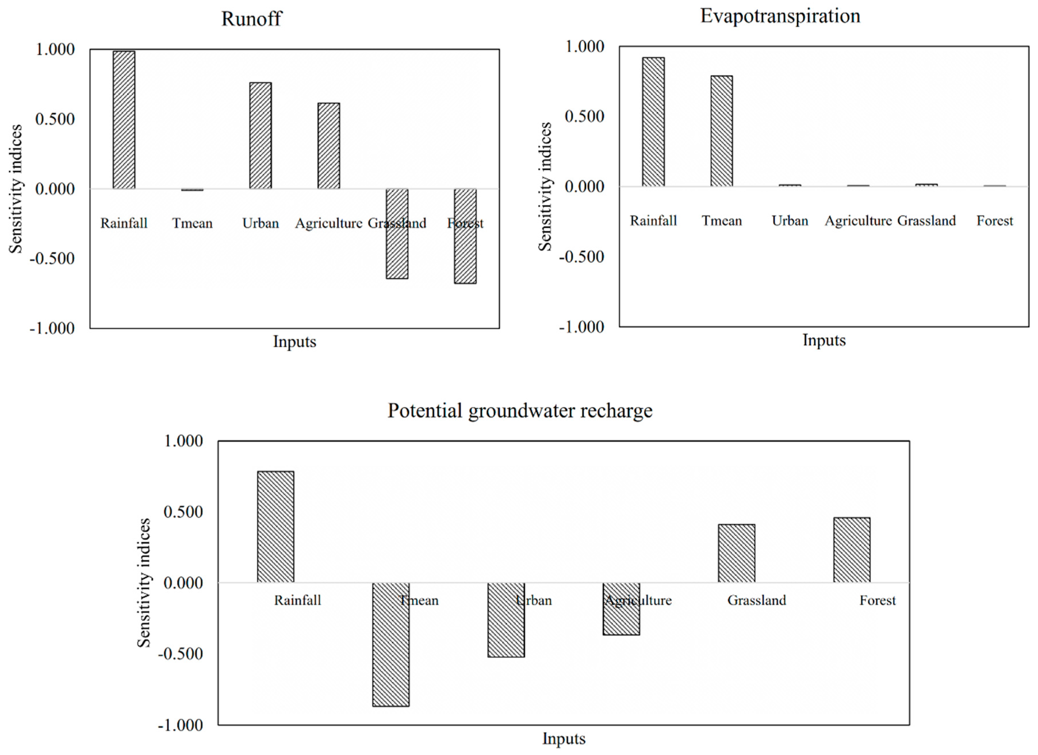
Water balance is sensitive to the changes in climatological data and basin conditions, which is, in this case, changing LULC. Increasing urban and agricultural LULC accelerates the rate at which $R_u$ is rising. Because the percentage of the region that has urbanized is small compared to the other LULC categories, the $R_u$ contribution of urban areas is small. T_mean, urban, and agricultural covers are inversely related to R_e, indicating that increases of this factors could lead to reductions in R_e in the study area. Considering that ET is one of the parameters with a higher weighting in the water balance and LULC changes, it also induce changes in ET rates. For every LULC category, changes are inversely related to ET: increasing urban areas can decrease ET and decreasing forestland also decreases ET, as mentioned above. Less ET means more R_u and increases the likelihood of Re [46]. ET was not calculated for forest, urban, and grassland land uses and was not included in the analysis. This a limitation of the method because it is a limited consideration of the impacts of the other three LULCs. This underestimates the real effect of LULC on ET in the study. This could be the basis for future research that more closely examines the relationships between LULCs and ET in the study area.

Sensitivity analysis with the empirical values measured at the five meteorological stations (139 inputs) is not sensitive to changing forest area because it has not changed much in the study area, and results will indicate that increases in forest will produce increases in runoff. Nevertheless, ET sensitivity analysis indicate that increase in urban areas and decrease in forestland can promote R_e (PRCC values of −0.1222 and 0.002 for urban and forestland), but these values are not significant. Similar values are found in Minnig, et al. [45] and it can most likely explain the R_e trend from 1986 to 2013, which increases by 72.29 mm/year.

Changing Water Tables and Depleting Aquifers

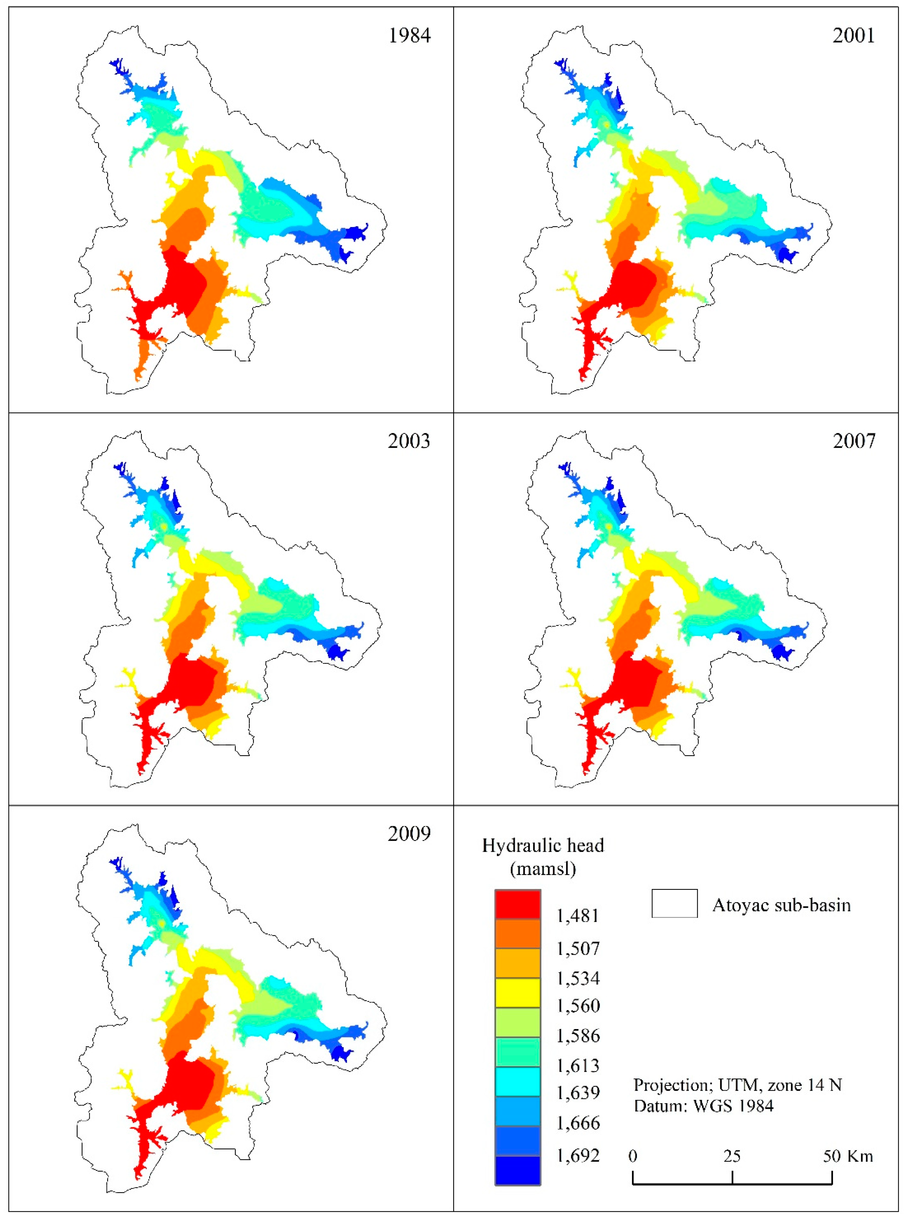
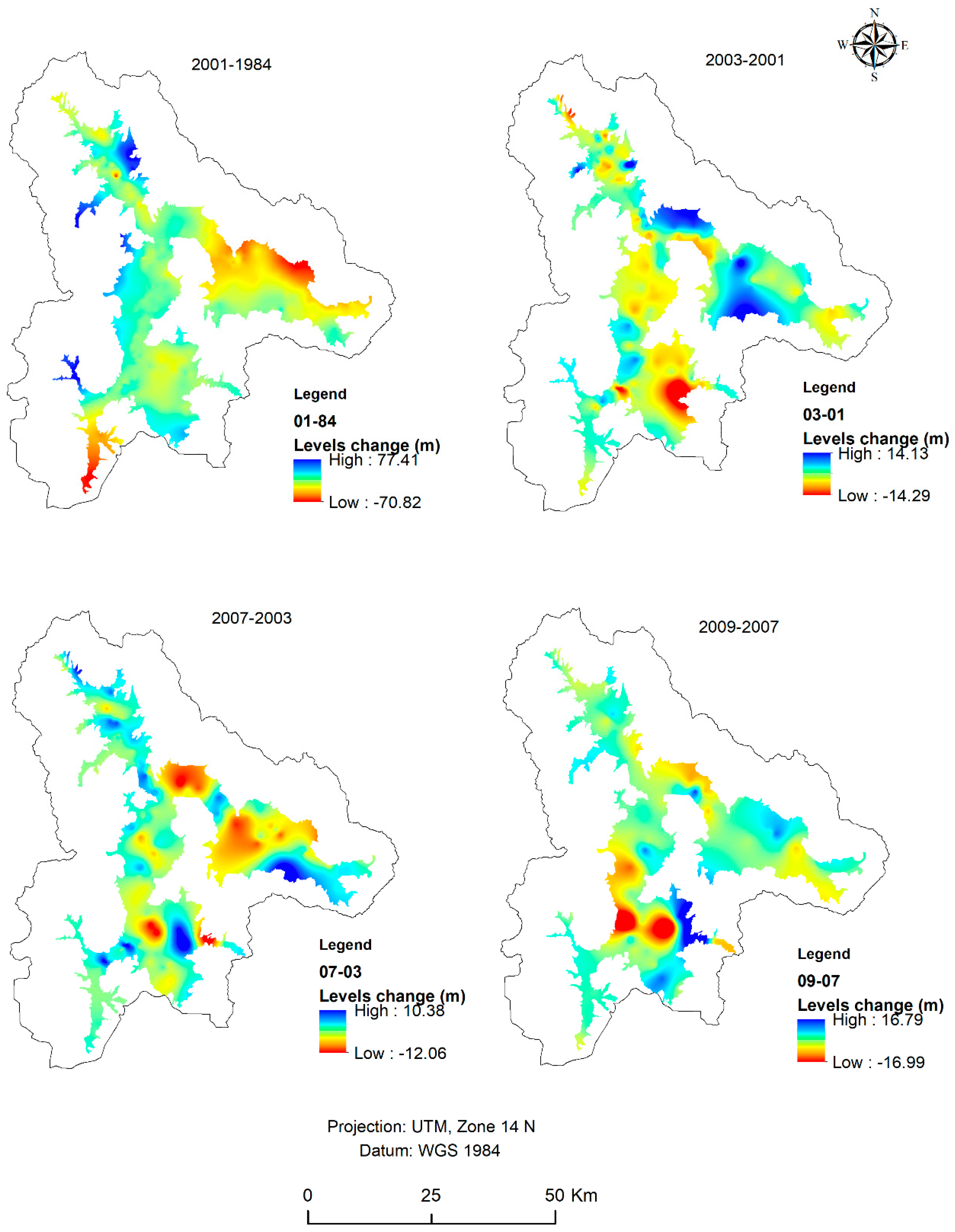
Since 1984, depletion cones have become apparent throughout the sub-basin. Over the last 25 years, the Tlacolula Valley’s water table has fallen 38 m. In the Etla Valley, the aquifer has fallen between 29 m and 44 m. In the Zaachila Valley, the depletion is 25 m. There is constant pressure upon the groundwater, which is evident by what the annual extraction volume has done to the hydraulic head. The extracted volume in 1984 was 115.53 × 10⁶ m³ and in 2009 it was 331.8 × 10⁶ m³. By 2009, the extraction rate surpassed the annual R_e rate of 169 × 10⁶ m³ [22]. Over the same period, consumption nearly doubled from 47.54 × 10⁶ m³ in 1984 to 80.04 × 10⁶ m³ in 2009 (a calculation based on an average water demand of 216 LPD). This depletion is due to CC, intensified T, urbanization, and the increasing extent of impervious surfaces. Consumers of water in the study area are extracting more water from the aquifer than is available to R_e due to increasing $R_u$ and higher ET.

There is relationship between urbanization and water consumption since the latter is tied to population growth. The negative effects of population on water resources are numerous [10], as the water input into the aquifer has diminished and the water demand for different uses increases. If continued, a 2.3% annual population growth rate will cause great pressure on water resources over the coming decades; this is borne out by the projections examined here. One potential solution that can be inferred from the projections is to reduce water consumption to a per-person average of less than 50 LPD.

Water is a particularly vital resource in this region. It is the engine of the economy in both urban and rural areas which are based on small business, tourism, agriculture, forestry, and ecotourism. In the last decade, insufficient water supplies have become notorious, but research on this problem has been very limited. It can be said that economic activities and population growth have increased environmental problems by the overexploitation of groundwater over the last 25 years. Some scholars have indicated that groundwater exploitation has yielded economic growth around the world over the last five decades, but it has also yielded significant social and environmental costs [69,70]. One future consequence that may arise in the area due to overexploitation of groundwater is subsidence of land surfaces; this is already happening in some regions of Mexico due to overexploitation of aquifers [71,72,73].

5. Conclusions

Over the 34-year period of analysis, water recharge in the study area has been driven primarily by climatological conditions in the sub-basin, especially the variations in rainfall and temperature, which are the main variables of the water balance calculation. There has been little change in the proportions of LULC categories; only urban area has increased significantly due to population growth over the last three decades. Runoff from urban areas increased, but the change was relatively small, from 1.45% in 1986 to 4.84% 2018. Thus, although urban areas increased in size and runoff amount, the largest contribution still comes from agricultural areas. Agricultural land use comprises 31% of the total sub-basin. Together, the impacts of agriculture and urban land use demonstrate the direct impact of human activities on groundwater resources in the Central Valleys of Oaxaca: population growth leads to increasing abstraction of continuously shrinking supplies of groundwater.

Groundwater is a high-risk resource due to fluctuating R_e rates and human activities. High levels of exploitation put all users into precarious positions, and this is demonstrated by the projections of future groundwater supplies and trends in groundwater extraction. The main threats in the Alto Atoyac sub-basin are CC, LULC change, and population growth.

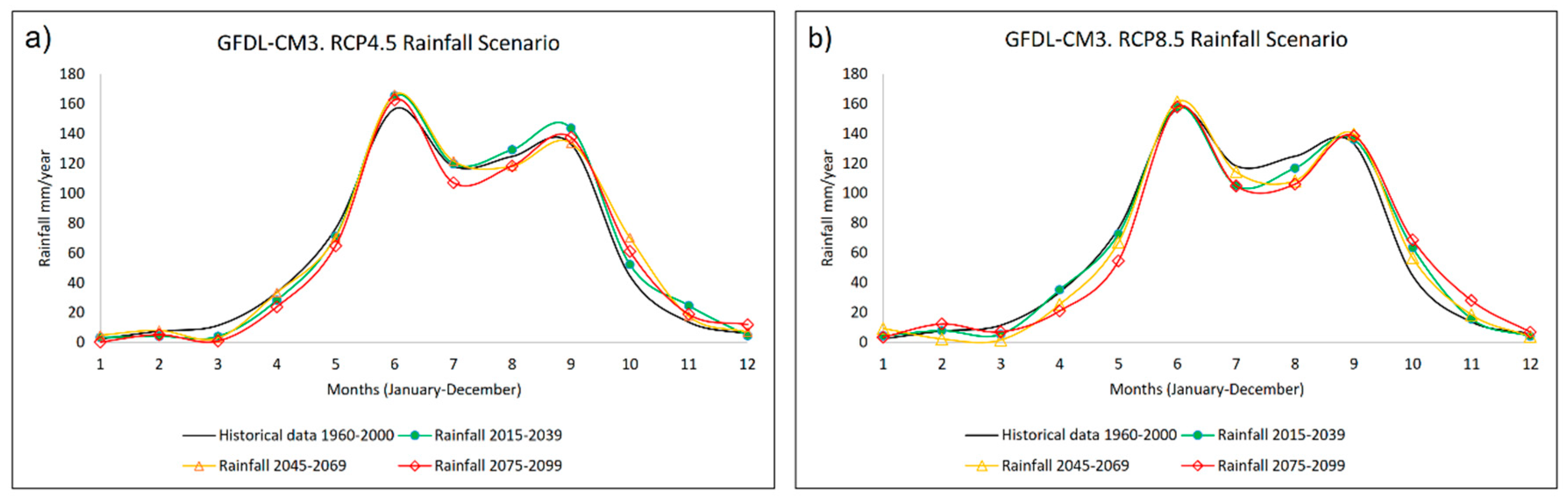
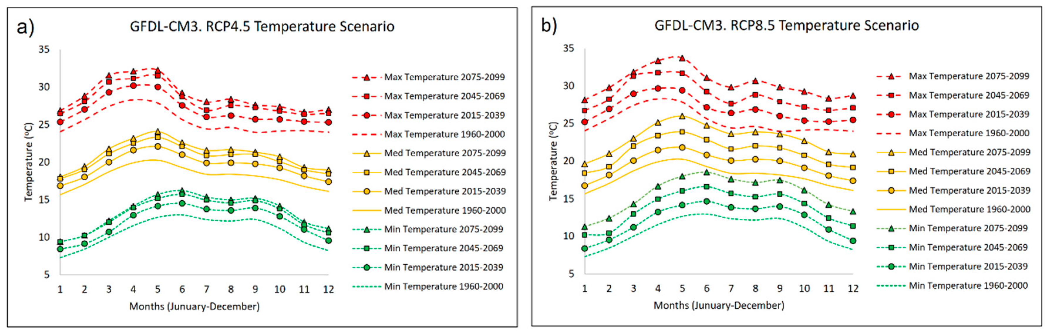
Climate data indicate that despite increases in annual P, rising average annual T and increasing ET rates will produce diminishing R_e of groundwater resources for the future. According to the RCP4.5 climate-change scenario, mean annual T is projected to increase over the near, middle, and distant future by 1.46 °C, 2.49 °C, and 3.02 °C, respectively. This is likely to intensify ET rates by 1.86%, 3.49%, and 5.56%, respectively. The increases of 1.49 °C, 3.21 °C, and 4.95 °C projected by the RCP8.5 model will yield increases of 2.78%, 5.97%, and 8.18% in ET rates.

LULC change and shifting patterns of T are the main influencers of the water R_e changes. Increasing T and urbanization enhance both ET and $R_u$ and allow for less potential R_e of aquifers. From 1986 to 2018, mean annual T increased 1.76 °C and the urban LULC increased 2.3 km²/year. Projections under the RCP4.5 and RCP8.5 scenarios show that the R_e rate will diminish to the first horizon by 35.48% and 44.47 %, respectively. At the most distant horizons of both scenarios, potential R_e is projected to decrease 67.69% (RCP4.5) and 86.56% (RCP8.5), indicating that there will be groundwater availability problems in the future.

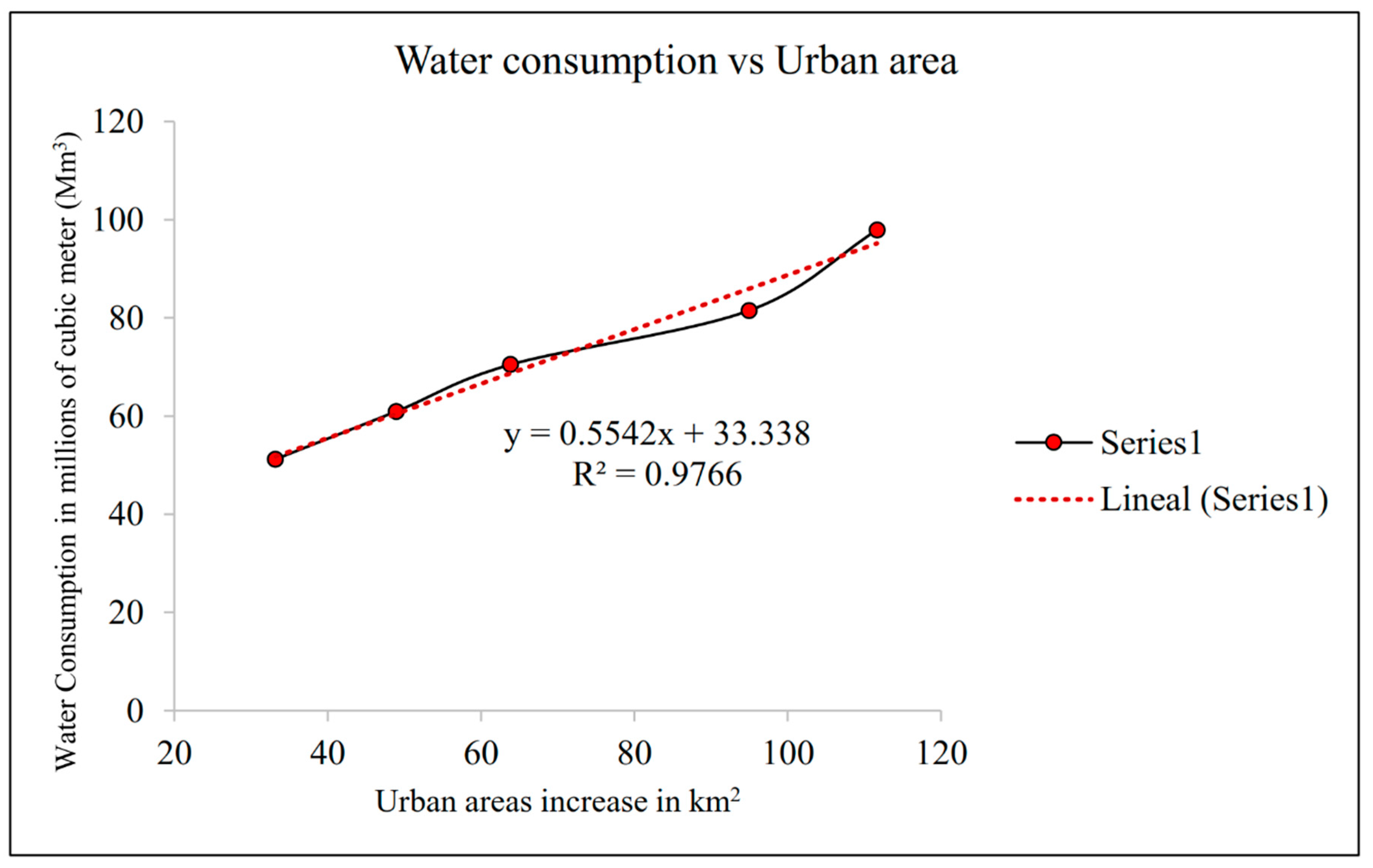
As urban areas increase, population will increase and so will the demand for fresh water. There will be a negative consequence on groundwater because of the concomitant increased $R_u$ and magnified extraction of groundwater to meet basic needs. From 1986 to 2018, $R_u$ increased at a rate of 0.24 mm/year in urban areas. The $R_u$ in the urban portions of the study area, which are only 2.86% of the total area, increased by 236% (from 1986 to 2018). Water demand grew from 47.54 × 10⁶ m³ to 97.93 × 10⁶ m³ for the same period, which clearly demonstrates the implications of urbanization and population growth for water supplies.

Water balance is sensitive to climate variation, indicating the effects that CC can have in the study area. Physical changes consequential to LULC change have significant effects on the water balance, too. Increases of urban and agricultural areas can generate inverse changes of R_e, and they can generate negative consequences in the future. Agricultural areas are expected to shrink in the area due to farm abandonment and urban expansion into rural areas.

Groundwater volumes are being depleted at a rate of 284.34 × 10⁶ m³/year, a deficit of 115.34 × 10⁶ m³/year (a reduction in the groundwater levels of 0.1 m/year). This is consistent with the increased water demand of the last few years and with reduced R_e stemming from changing LULC and increasing T.

Some ways to confront these challenges could be to strategically protect R_e zones from urbanization, to undertake small-scale engineering projects that enhance R_e rates in areas prone to $R_u$, and to reduce water consumption rates throughout the basin to below 50 LPD to ease the pressure upon the region’s groundwater resources.

References

1. Arnell, N.W. Climate change and global water resources. Glob. Environ. Chang. 1999, 9, S31–S49. [Google Scholar] [CrossRef]
2. Winter, T.C. The concept of hydrologic landscapes. J. Am. Water Resour. Assoc. 2001, 37, 335–349. [Google Scholar] [CrossRef]
3. Gleeson, T.; Wada, Y.; Bierkens, M.F.P.; van Beek, L.P.H. Water balance of global aquifers revealed by groundwater footprint. Nature 2012, 488, 197. [Google Scholar] [CrossRef] [PubMed]
4. Jakeman, A.J.; Barreteau, O.; Hunt, R.J.; Rinaudo, J.-D.; Ross, A.; Arshad, M.; Hamilton, S. Integrated Groundwater Management: An Overview of Concepts and Challenges. In Integrated Groundwater Management: Concepts, Approaches and Challenges; Jakeman, A.J., Barreteau, O., Hunt, R.J., Rinaudo, J.-D., Ross, A., Eds.; Springer International Publishing: Cham, Switzerland, 2016; pp. 3–20. [Google Scholar] [Green Version]
5. Siebert, S.; Burke, J.; Faures, J.M.; Frenken, K.; Hoogeveen, J.; Döll, P.; Portmann, F.T. Groundwater use for irrigation—A global inventory. Hydrol. Earth Syst. Sci. 2010, 14, 1863–1880. [Google Scholar] [CrossRef]
6. Lejars, C.; Fusillier, J.L.; Bouarfa, S.; Coutant, C.; Brunel, L.; Rucheton, G. Limitation of agricultural groundwater uses in beauce (france): what are the impacts on farms and on the food-processing sector? Irrig. Drain. 2012, 61, 54–64. [Google Scholar] [CrossRef]
7. Shahid, S.; Wang, X.-J.; Rahman, M.M.; Hasan, R.; Harun, S.B.; Shamsudin, S. Spatial assessment of groundwater over-exploitation in northwestern districts of Bangladesh. J. Geol. Soc. India 2015, 85, 463–470. [Google Scholar] [CrossRef] [Green Version]
8. Sharma, K.D. Groundwater management for food security. Curr. Sci. 2009, 96, 1444–1447. [Google Scholar]
9. Mekonnen, M.M.; Hoekstra, A.Y. Four billion people facing severe water scarcity. Sci. Adv. 2016, 2, e1500323. [Google Scholar] [CrossRef] [PubMed]
10. Vörösmarty, C.J.; Green, P.; Salisbury, J.; Lammers, R.B. Global water resources: Vulnerability from climate change and population growth. Science 2000, 289, 284–288. [Google Scholar] [CrossRef] [PubMed]
11. Vörösmarty, C.J.; McIntyre, P.B.; Gessner, M.O.; Dudgeon, D.; Prusevich, A.; Green, P.; Glidden, S.; Bunn, S.E.; Sullivan, C.A.; Liermann, C.R.; et al. Global threats to human water security and river biodiversity. Nature 2010, 467, 555. [Google Scholar] [CrossRef] [PubMed]
12. Wada, Y.; van Beek, L.P.H.; van Kempen, C.M.; Reckman, J.W.T.M.; Vasak, S.; Bierkens, M.F.P. Global depletion of groundwater resources. Geophys. Res. Lett. 2010, 37. [Google Scholar] [CrossRef] [Green Version]
13. Taylor, R.G.; Scanlon, B.; Döll, P.; Rodell, M.; van Beek, R.; Wada, Y.; Longuevergne, L.; Leblanc, M.; Famiglietti, J.S.; Edmunds, M.; et al. Ground water and climate change. Nat. Clim. Chang. 2012, 3, 322. [Google Scholar] [CrossRef]
14. Dalin, C.; Wada, Y.; Kastner, T.; Puma, M.J. Groundwater depletion embedded in international food trade. Nature 2017, 543, 700. [Google Scholar] [CrossRef] [PubMed]
15. Bhat, V.; Prajwal, M.; Shetty, A.; Srivastava, A.; Bhosale, R. Spatiotemporal Relationship Linking Land Use/Land Cover with Groundwater Level. In Groundwater; Springer: Singapore, 2018; pp. 41–54. [Google Scholar]
16. Delhomme, J.P. Kriging in the hydrosciences. Adv. Water Resour. 1978, 1, 251–266. [Google Scholar] [CrossRef]
17. Aboufirassi, M.; Mariño, M.A. Kriging of water levels in the Souss aquifer, Morocco. J. Int. Assoc. Math. Geol. 1983, 15, 537–551. [Google Scholar] [CrossRef]
18. Boken, V.K.; Hoogenboom, G.; Hook, J.E.; Thomas, D.L.; Guerra, L.C.; Harrison, K.A. Agricultural water use estimation using geospatial modeling and a geographic information system. Agric. Water Manag. 2004, 67, 185–199. [Google Scholar] [CrossRef]
19. Starr, G.C. Assessing temporal stability and spatial variability of soil water patterns with implications for precision water management. Agric. Water Manag. 2005, 72, 223–243. [Google Scholar] [CrossRef]
20. Arslan, H. Spatial and temporal mapping of groundwater salinity using ordinary kriging and indicator kriging: The case of Bafra Plain, Turkey. Agric. Water Manag. 2012, 113, 57–63. [Google Scholar] [CrossRef]
21. Kang, R.; Kaur, D. Spatial pattern of ground water level changes in the irrigated agricultural region of Bist Doab, Punjab, India. Singap. J. Trop. Geogr. 2017, 39, 75–89. [Google Scholar] [CrossRef]
22. Ojeda Olivares, E.A.; Belmonte Jimenez, S.I.; Takaro, T.K.; Campos Enriquez, J.O.; Ladrón de Guevara Torres, M. Decrease of the water recharge and identification of water recharge zones in the Alto Atoyac sub-basin, Oaxaca, as a result of climate change. J. Water Clim. Chang. 2017, 9, 37–57. [Google Scholar] [CrossRef]
23. Campos-Enríquez, J.O.; Belmonte-Jiménez, S.I.; Keppie, J.D.; Ortega-Gutiérrez, F.; Arzate, J.A.; Martínez-Silva, J.; Martínez-Serrano, R.G. Gravity and magnetic survey of the Oaxaca city region: Cenozoic horst-and-graben structure superimposed on the Oaxaca—Juarez terrane boundary, southern Mexico. J. S. Am. Earth Sci. 2010, 29, 572–585. [Google Scholar] [CrossRef]
24. Campos-Enriquez, J.O.; Corbo-Camargo, F.; Arzate-Flores, J.; Keppie, J.D.; Arango-Galván, C.; Unsworth, M.; Belmonte-Jiménez, S.I. The buried southern continuation of the Oaxaca-Juarez terrane boundary and Oaxaca Fault, southern Mexico: Magnetotelluric constraints. J. S. Am. Earth Sci. 2013, 43, 62–73. [Google Scholar] [CrossRef]
25. Clarke, L.; Edmonds, J.; Jacoby, H.; Pitcher, H.; Reilly, J.; Richels, R. CCSP Synthesis and Assessment Product 2.1, Part A: Scenarios of Greenhouse Gas Emissions and Atmospheric Concentrations; US Government Printing Office: Washington, DC, USA, 2007.
26. Thomson, A.M.; Calvin, K.V.; Smith, S.J.; Kyle, G.P.; Volke, A.; Patel, P.; Delgado-Arias, S.; Bond-Lamberty, B.; Wise, M.A.; Clarke, L.E.; et al. RCP4.5: A pathway for stabilization of radiative forcing by 2100. Clim. Chang. 2011, 109, 77. [Google Scholar] [CrossRef]
27. Riahi, K.; Rao, S.; Krey, V.; Cho, C.; Chirkov, V.; Fischer, G.; Kindermann, G.; Nakicenovic, N.; Rafaj, P. RCP 8.5—A scenario of comparatively high greenhouse gas emissions. Clim. Chang. 2011, 109, 33. [Google Scholar] [CrossRef]
28. Fernández Eguiarte, A.; Zavala, J.; Romero, R.; Conde, C.; Trejo, R. Actualización de Los Escenarios de Cambio Climático Para Estudios de Impactos, Vulnerabilidad Y Adaptación en México Y Centroamérica; Centro de Ciencias de la Atmósfera, Universidad Nacional Autónoma de México: Mexico City, Mexico, 2015. [Google Scholar]
29. Schroeder, P.R.; Aziz, N.; Lloyd, C.; Zappi, P. The Hydrologic Evaluation of Landfill Performance (HELP) Model: User’s Guide for Version 3; EPA/600/R-94/168a; U.S. Environmental Protection Agency Office of Research and Development: Washington, DC, USA, 1994.
30. Berger, K.; Schroeder, P. The Hydrologic Evaluation of Landfill Performance (HELP) Model: User’s Guide for HELP-D (Version 3.95 D). In 6th Revised Edition for Version HELP 3.95D; Institute of Soil Science, University of Hamburg: Hamburg, Germany, 2013; p. 74. [Google Scholar]
31. Breiman, L. Random forests. Mach. Learn. 2001, 45, 5–32. [Google Scholar] [CrossRef]
32. Fitzpatrick-Lins, K. Comparison of sampling procedures and data analysis for a land-use and land-cover map. Photogramm. Eng. Remote Sens. 1981, 47, 343–351. [Google Scholar]
33. SCS. SCS National Engineering Handbook, Section 4: Hydrology; United States Department of Agriculture, Soil Conservation Service: Washington, DC, USA, 1985.
34. Wagener, T.; Kollat, J. Numerical and visual evaluation of hydrological and environmental models using the Monte Carlo analysis toolbox. Environ. Model. Softw. 2007, 22, 1021–1033. [Google Scholar] [CrossRef]
35. Saltelli, A.; Tarantola, S.; Campolongo, F.; Ratto, M. Sensitivity Analysis in Practice: A Guide to Assessing Scientific Models; Wiley: Chichester, UK, 2004. [Google Scholar]
36. Kovoor, G.M.; Nandagiri, L. Sensitivity Analysis of FAO-56 Penman–Monteith Reference Evapotranspiration Estimates Using Monte Carlo Simulations. In Hydrologic Modeling; Springer: Singapore, 2018; pp. 73–84. [Google Scholar]
37. Singh, C.K.; Katpatal, Y.B. Spatial and Temporal Variations of Groundwater Level: A Case Study of Wainganga Sub-basin, Nagpur, India. In Groundwater; Springer: Singapore, 2018; pp. 21–30. [Google Scholar]
38. INEGI. VALLES CENTRALES DE OAXACA PERFIL SOCIODEMOGRAFICO XI CENSO GENERAL DE POBLACION Y VIVIENDA, 1990; INEGI: Aguas Calientes, Mexico, 1993; p. 66.
39. INEGI. Censo de Población Y Vivienda 2010. Available online: https://www.inegi.org.mx/programas/ccpv/2010/default.html#Publicaciones (accessed on 27 September 2018).
40. CNA. Situacion del Subsector Agua Potable, Alcantarillado Y Saneamiento; CONAGUA: Coyoacan, Mexico, 2010; p. 81. [Google Scholar]
41. Gosling, S.N.; Arnell, N.W. A global assessment of the impact of climate change on water scarcity. Clim. Chang. 2016, 134, 371–385. [Google Scholar] [CrossRef]
42. Veldkamp, T.; Wada, Y.; Ward, P.; Aerts, J. Impacts of land use and land cover change on water resources and water scarcity in the 20th century: A multi-model multi-forcing analysis. In Proceedings of the EGU General Assembly Conference Abstracts, Vienna, Austria, 17–22 April 2016. [Google Scholar]
43. Mathews, A.S. Suppressing Fire and Memory: Environmental Degradation and Political Restoration in the Sierra Juárez of Oaxaca, 1887–2001. Environ. Hist. 2003, 8, 77–108. [Google Scholar] [CrossRef]
44. Robson, J.P.; Berkes, F. Exploring some of the myths of land use change: Can rural to urban migration drive declines in biodiversity? Glob. Environ. Chang. 2011, 21, 844–854. [Google Scholar] [CrossRef]
45. Minnig, M.; Moeck, C.; Radny, D.; Schirmer, M. Impact of urbanization on groundwater recharge rates in Dübendorf, Switzerland. J. Hydrol. 2018, 563, 1135–1146. [Google Scholar] [CrossRef]
46. Nan, Y.; Bao-hui, M.; Chun-kun, L. Impact Analysis of Climate Change on Water Resources. Procedia Eng. 2011, 24, 643–648. [Google Scholar] [CrossRef] [Green Version]
47. Arnell, N.W.; Lowe, J.A.; Brown, S.; Gosling, S.N.; Gottschalk, P.; Hinkel, J.; Lloyd-Hughes, B.; Nicholls, R.J.; Osborn, T.J.; Osborne, T.M.; et al. A global assessment of the effects of climate policy on the impacts of climate change. Nat. Clim. Chang. 2013, 3, 512. [Google Scholar] [CrossRef]
48. Collins, M.; Knutti, R.; Arblaster, J.; Dufresne, J.-L.; Fichefet, T.; Friedlingstein, P.; Gao, X.; Gutowski, W.J.; Johns, T.; Krinner, G.; et al. Chapter 12- Long-term climate change: Projections, commitments and irreversibility. In Climate Change 2013: The Physical science Basis. IPCC Working Group I Contribution to AR5; Cambrigde University Press: Cambridge, UK, 2013. [Google Scholar]
49. Peterson, T.C.; Hoerling, M.P.; Stott, P.A.; Herring, S.C. Explaining Extreme Events of 2012 from a Climate Perspective. Bull. Am. Meteorol. Soc. 2013, 94, S1–S74. [Google Scholar] [CrossRef] [Green Version]
50. Afshar, N.R.; Fahmi, H. Impact of climate change on water resources in Iran. Int. J. Energy Water Resour. 2019, 3, 55–60. [Google Scholar] [CrossRef]
51. Fischer, E.M.; Knutti, R. Observed heavy precipitation increase confirms theory and early models. Nat. Clim. Chang. 2016, 6, 986. [Google Scholar] [CrossRef]
52. Prein, A.F.; Rasmussen, R.M.; Ikeda, K.; Liu, C.; Clark, M.P.; Holland, G.J. The future intensification of hourly precipitation extremes. Nat. Clim. Chang. 2016, 7, 48. [Google Scholar] [CrossRef]
53. Pendergrass, A.G.; Knutti, R.; Lehner, F.; Deser, C.; Sanderson, B.M. Precipitation variability increases in a warmer climate. Sci. Rep. 2017, 7, 17966. [Google Scholar] [CrossRef]
54. Wang, G.; Wang, D.; Trenberth, K.E.; Erfanian, A.; Yu, M.; Bosilovich, M.G.; Parr, D.T. The peak structure and future changes of the relationships between extreme precipitation and temperature. Nat. Clim. Chang. 2017, 7, 268. [Google Scholar] [CrossRef]
55. Trenberth, K.E.; Dai, A.; Rasmussen, R.M.; Parsons, D.B. The Changing Character of Precipitation. Bull. Am. Meteorol. Soc. 2003, 84, 1205–1218. [Google Scholar] [CrossRef]
56. Watson, J.E.M.; Iwamura, T.; Butt, N. Mapping vulnerability and conservation adaptation strategies under climate change. Nat. Clim. Chang. 2013, 3, 989. [Google Scholar] [CrossRef]
57. Henrichs, M.; Steinbrich, A.; Leistert, H.; Scherer, I.; Schuetz, T.; Uhl, M.; Weiler, M. Model Based Estimation of a Natural Water Balance as Reference for Planning in Urban Areas. Available online: https://link.springer.com/chapter/10.1007/978-3-319-99867-1_164 (accessed on 27 September 2018).
58. Zhang, L.; Cheng, L.; Chiew, F.; Fu, B. Understanding the impacts of climate and landuse change on water yield. Curr. Opin. Environ. Sustain. 2018, 33, 167–174. [Google Scholar] [CrossRef]
59. Ferreira, C.S.S.; Walsh, R.P.D.; Ferreira, A.J.D. Degradation in urban areas. Curr. Opin. Environ. Sci. Health 2018, 5, 19–25. [Google Scholar] [CrossRef] [Green Version]
60. Sajikumar, N.; Remya, R.S. Impact of land cover and land use change on runoff characteristics. J. Environ. Manag. 2015, 161, 460–468. [Google Scholar] [CrossRef] [PubMed]
61. Zipper, S.C.; Soylu, M.E.; Kucharik, C.J.; Loheide, S.P., II. Quantifying indirect groundwater-mediated effects of urbanization on agroecosystem productivity using MODFLOW-AgroIBIS (MAGI), a complete critical zone model. Ecol. Model. 2017, 359, 201–219. [Google Scholar] [CrossRef]
62. Locatelli, L.; Mark, O.; Mikkelsen, P.S.; Arnbjerg-Nielsen, K.; Deletic, A.; Roldin, M.; Binning, P.J. Hydrologic impact of urbanization with extensive stormwater infiltration. J. Hydrol. 2017, 544, 524–537. [Google Scholar] [CrossRef] [Green Version]
63. Wakode, H.B.; Baier, K.; Jha, R.; Azzam, R. Impact of urbanization on groundwater recharge and urban water balance for the city of Hyderabad, India. Int. Soil Water Conserv. Res. 2018, 6, 51–62. [Google Scholar] [CrossRef]
64. Qiu, G.-Y.; Li, H.-Y.; Zhang, Q.-T.; Chen, W.; Liang, X.-J.; Li, X.-Z. Effects of Evapotranspiration on Mitigation of Urban Temperature by Vegetation and Urban Agriculture. J. Integr. Agric. 2013, 12, 1307–1315. [Google Scholar] [CrossRef]
65. Bagley, J.E.; Desai, A.R.; Harding, K.J.; Snyder, P.K.; Foley, J.A. Drought and Deforestation: Has Land Cover Change Influenced Recent Precipitation Extremes in the Amazon? J. Clim. 2013, 27, 345–361. [Google Scholar] [CrossRef]
66. Desbureaux, S.; Damania, R. Rain, forests and farmers: Evidence of drought induced deforestation in Madagascar and its consequences for biodiversity conservation. Biol. Conserv. 2018, 221, 357–364. [Google Scholar] [CrossRef]
67. Nazareno, A.G.; Laurance, W.F. Brazil’s drought: Beware deforestation. Science 2015, 347, 1427. [Google Scholar] [CrossRef] [PubMed]
68. Shukla, J.; Nobre, C.; Sellers, P. Amazon Deforestation and Climate Change. Science 1990, 247, 1322. [Google Scholar] [CrossRef]
69. Custodio, E. Aquifer overexploitation: What does it mean? Hydrogeol. J. 2002, 10, 254–277. [Google Scholar] [CrossRef]
70. Birol, E.; Koundouri, P.; Kountouris, Y. Assessing the economic viability of alternative water resources in water-scarce regions: Combining economic valuation, cost-benefit analysis and discounting. Ecol. Econ. 2010, 69, 839–847. [Google Scholar] [CrossRef] [Green Version]
71. Castellazzi, P.; Martel, R.; Rivera, A.; Huang, J.; Pavlic, G.; Calderhead, A.I.; Chaussard, E.; Garfias, J.; Salas, J. Groundwater depletion in Central Mexico: Use of GRACE and InSAR to support water resources management. Water Resour. Res. 2016, 52, 5985–6003. [Google Scholar] [CrossRef]
72. Castellazzi, P.; Arroyo-Domínguez, N.; Martel, R.; Calderhead, A.I.; Normand, J.C.L.; Gárfias, J.; Rivera, A. Land subsidence in major cities of Central Mexico: Interpreting InSAR-derived land subsidence mapping with hydrogeological data. Int. J. Appl. Earth Obs. Geoinf. 2016, 47, 102–111. [Google Scholar] [CrossRef]
73. Castellazzi, P.; Garfias, J.; Martel, R.; Brouard, C.; Rivera, A. InSAR to support sustainable urbanization over compacting aquifers: The case of Toluca Valley, Mexico. Int. J. Appl. Earth Obs. Geoinf. 2017, 63, 33–44. [Google Scholar] [CrossRef]
Figure 1. Location of the study area in the Central Valleys of Oaxaca.
Remotesensing 11 01290 g001
Figure 2. Soil type and hydraulic conductivity distribution.
Remotesensing 11 01290 g002
Figure 3. Climographs of five meteorological stations in the study area.
Remotesensing 11 01290 g003
Figure 4. (a,b) Normal monthly P for historical and future climate projections under RCP4.5 and RCP 8.5 for 2015–2039, 2045–2069, and 2075–2099 horizons modeled by GFDL-CM3.
Remotesensing 11 01290 g004
Figure 5. (a,b) Normal monthly T for historical and future climate projections under RCP4.5 and RCP 8.5 for 2015–2039, 2045–2069, and 2075–2099 horizons modeled by GFDL-CM3.
Remotesensing 11 01290 g005
Figure 6. Piezometric head (in m) in the Central Valleys of Oaxaca during the dry seasons of 1984, 2001, 2003, 2007, and 2009.
Remotesensing 11 01290 g006
Figure 7. Volume storage change (in m) in the Central Valleys of Oaxaca during the dry seasons of 1984, 2001, 2003, 2007, and 2009.
Remotesensing 11 01290 g007
Figure 8. Sensitivity indices for water balance variables in the study area.
Remotesensing 11 01290 g008
Figure 9. Relationship between urban growth and water consumption (Mm3).
Remotesensing 11 01290 g009