Article

Estimation of Translational Motion Parameters in Terahertz Interferometric Inverse Synthetic Aperture Radar (InISAR) Imaging Based on a Strong Scattering Centers Fusion Technique

College of Electronic Science and Technology, National University of Defense Technology, Changsha 410073, China
*
Author to whom correspondence should be addressed.
Remote Sens. 2019, 11(10), 1221; https://doi.org/10.3390/rs11101221
Submission received: 25 April 2019 / Revised: 14 May 2019 / Accepted: 20 May 2019 / Published: 23 May 2019
(This article belongs to the Special Issue Radar and Sonar Imaging and Processing)

Abstract

:
Translational motion of a target will lead to image misregistration in interferometric inverse synthetic aperture radar (InISAR) imaging. In this paper, a strong scattering centers fusion (SSCF) technique is proposed to estimate translational motion parameters of a maneuvering target. Compared to past InISAR image registration methods, the SSCF technique is advantageous in its high computing efficiency, excellent antinoise performance, high registration precision, and simple system structure. With a one-input three-output terahertz InISAR system, translational motion parameters in both the azimuth and height direction are precisely estimated. Firstly, the motion measurement curves are extracted from the spatial spectrums of mutually independent strong scattering centers, which avoids the unfavorable influences of noise and the “angle scintillation” phenomenon. Then, the translational motion parameters are obtained by fitting the motion measurement curves with phase unwrapping and intensity-weighted fusion processing. Finally, ISAR images are registered precisely by compensating the estimated translational motion parameters, and high-quality InISAR imaging results are achieved. Both simulation and experimental results are used to verify the validity of the proposed method.

Graphical Abstract

1. Introduction

Historically, the application of inverse synthetic aperture radar (ISAR) imaging in target recognition is limited, owing to the fact that the technique only captures the projected two-dimensional (2-D) characteristics of the target. To overcome this drawback, interferometric ISAR (InISAR) that provides three-dimensional (3-D) information of the target has been developed [1,2,3,4,5,6,7,8,9,10,11]. InISAR systems are generally composed of several fixed channels, with one as both a transmitter and receiver and the rest as full-time receivers. The 3-D geometry of the target can be reconstructed based on the phase difference of different ISAR images. Until now, nearly all researches regarding InISAR imaging have been carried out in the microwave band, while limited research about InISAR imaging with terahertz (THz) radars is available in the current literature. Compared to InISAR imaging with microwave radars, THz radars can more easily achieve a higher carrier frequency and wider absolute bandwidth, which provide higher spatial resolution and more detailed information of the target. Furthermore, THz InISAR imaging holds large potential in maneuvering target surveillance and recognition in space and near space, and it is of great significance to study and advance this technique.
With the noticeable progress of THz sources and detectors over the past few decades, it has become possible to achieve imaging and recognition with a THz radar system. For now, we can summarize the imaging radar system in the THz band into three main categories: raster-scanning radar system, mixed-scanning radar system, and an SAR/ISAR system. The raster-scanning radar system focuses the beam to a fixed area using several lenses, and the 3-D imaging result is obtained by recording the data of each scanning area. Representatives of such systems include Jet Propulsion Laboratory [12,13,14,15,16,17] and Pacific Northwest National Laboratory [18,19]. The imaging frame rate is determined by the number of scanning pixels and oscillation frequency of the scanning mirrors, which makes it time-consuming to obtain a target image. Besides, the system structure is complex and can be easily damaged. Compared to the raster-scanning radar system, the mixed-scanning radar system substitutes one-dimensional (1-D) raster scanning with 1-D electrical scanning or 1-D mechanical scanning, and the imaging speed can be greatly improved. Representatives of mixed-scanning radar systems include Chinese Academy of Sciences [20,21,22] and China Academy of Engineering Physics [23,24]. The mixed-scanning radar system can achieve 3-D imaging near real time, but some defects still exist (e.g., the imaging field of view is limited, and the target needs to be stationary). The SAR/ISAR system acquires the target image through relative motion between radar and target. The resolution depends on the bandwidth of the sweep signal and the length or relative rotation angle of the synthetic aperture. Representatives include FGAN-FHR [25,26,27], the US Defense Advanced Research Projects Agency (DARPA) [28], and so on [29,30,31,32,33]. Compared to the former two THz radar systems, the SAR/ISAR system has a relatively simple system structure and low hardware cost, and it has no limitation of target distance. However, the SAR/ISAR system can only achieve 2-D imaging. The THz InSAR/InISAR system has the advantages of the SAR/ISAR system and also has the ability to achieve 3-D imaging. Thus, it is meaningful to establish an InSAR/InISAR system in the THz band.
As we know, the translational motion of a target will lead to image misregistration in InISAR imaging, and an image registration process is necessary to be carried out first. In recent years, some research regarding image registration in InISAR systems have been presented. These image registration methods can be summarized into three categories. The first is based on the correlation coefficient of ISAR images such as the time domain correlation method and the frequency domain searching method [4]. However, in order to guarantee registration precision, the searching step of motion parameters should be controlled within a very limited range in the THz band, which significantly increases the computational complexity. The second is based on the selection of a reference distance, such as the respective reference distance compensation method and the reference distance deviation compensation method [5,6]. In these methods, the reference distance is chosen as the total distance from the transmitter to reference center and the reference center to corresponding receiver. There is no need to estimate the motion parameters, and the method is suitable for both three-antenna and multiantenna configurations. However, in a real InISAR imaging scene, it is highly challenging to acquire the accurate distances from the reference center to the other receivers (except the one as both a transmitter and receiver). The third is based on estimation of the motion parameters of target. Reference [7] presents a procedure based on a multiple antenna-pair InISAR imaging system with nine antennas to estimate angular motion parameters. The angular motion parameters measurement is based on the spatial spectrums of the whole target, and the phase wrapping of motion measurement curves is avoided by using a pair of antennas with a short baseline. However, there are some shortcomings in this method. Firstly, the multiple antenna-pair configuration increases the system complexity and hardware cost, especially in high-frequency applications. Secondly, the spatial spectrums in a fixed range cell usually contain information of several scattering centers, which would introduce the “angle glint” phenomenon to the motion measurement curves. Thirdly, the method does not consider the influence of noise, but the motion parameter measurement precision of the weak scattering centers is sensitive to noise. In addition to the limitations of the above methods, most research just gives the simulation results and are short on experimental validation.
Unlike SAR images, high-frequency ISAR images of moving targets usually consist of several dominating reflectors such as corner reflectors formed by the tail, fuselage, and wings of the aircraft. Taking the computing efficiency, practicability, robustness, and precision into consideration, a strong scattering centers fusion (SSCF) technique is proposed in this paper to estimate translational motion parameters using these dominating reflectors, which overcomes the defects in the aforementioned image registration methods. With a one-input three-output THz InISAR system, translational motion parameters both in the azimuth and height directions are accurately estimated. Strong scattering centers (SSCs) are extracted in the image domain with a rectangular filter operation, which eliminates most of the noise. Motion measurement curves are derived from the spatial spectrums of mutually independent SSCs so that the “angle scintillation” phenomenon can be effectively suppressed. Then, the translational motion parameters are obtained by fitting the motion measurement curves with phase unwrapping and intensity-weighted fusion processing. Finally, image registration is achieved by compensating the estimated motion parameters to the radar echoes, and the InISAR imaging results are obtained with a simple interference operation.
This paper is organized as follows: in Section 2, the signal model is established. The SSCF technique is described in detail in Section 3. In Section 4, the simulations of the point targets model under different signal-to-noise ratio (SNR) and equivalent verification experiments with a multichannel THz radar system are carried out. A discussion is given in Section 5. Conclusions are presented in in Section 6.

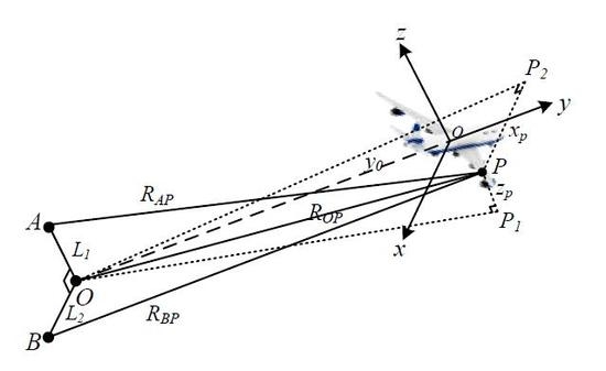
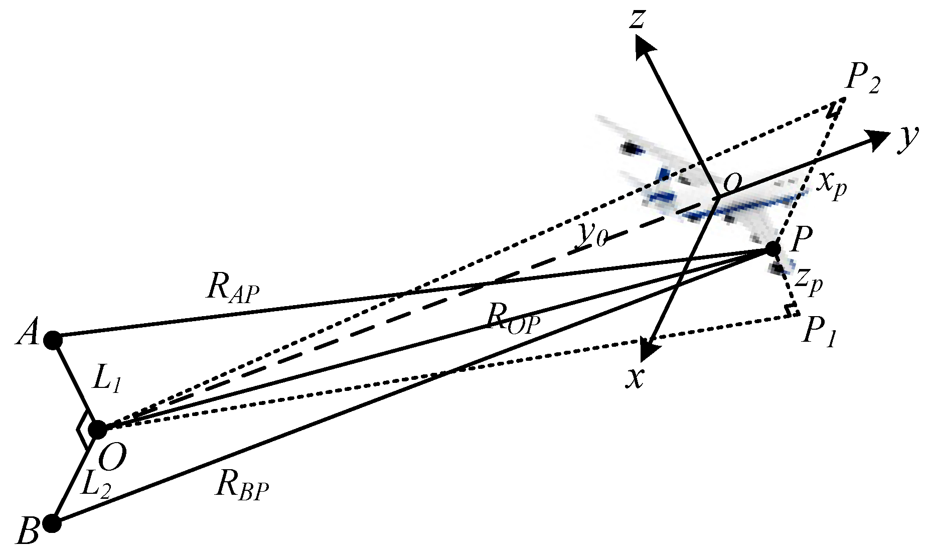
2. Signal Model of Interferometric Inverse Synthetic Aperture Radar (InISAR) Imaging

The configuration of the InISAR system is demonstrated in Figure 1. Antenna O acts as both the transmitter and receiver, while antennas A and B operate in the receiving mode only. L1 and L2 denote the lengths of the baselines OA and OB, respectively. A target coordinate system xoz is built referencing the right-angle layout of the three antennas. P ( x p , y p , z p ) is an arbitrary scattering center located on the target whose projections on planes xoy and yoz are P1 and P2, respectively. y 0 denotes the initial distance from antenna O to the reference center o, and R A P , R B P , and R O P denote the initial distances from P to three antennas, respectively. Suppose the transmitting linear frequency modulated (LFM) signal from antenna O is
s ( t ^ , t m ) = rect ( t ^ T p ) exp [ j 2 π ( f c t + γ t ^ 2 / 2 ) ] ,
where
rect ( u ) = { 1     | u | 0.5 0     | u | > 0.5 ,
then, T p is the pulse width, f c is the carrier frequency, γ is the chirp rate, t m is the slow time, t ^ is the fast time, and t = t m + t ^ is the full time.
Ignoring the signal envelope, the received signal at receiver i (i = O, A, B) from P is
s i ( t ^ , t m ) = σ P exp { j 2 π [ f c ( t R O P ( t ^ , t m ) + R i P ( t ^ , t m ) c ) + γ 2 ( t ^ R O P ( t ^ , t m ) + R i P ( t ^ , t m ) c ) 2 ] } ,
where c is the wave propagation velocity, σ P is the reflection coefficient of P, and R i P ( t ^ , t m ) represents the distance from receiver i to P at time t. These distances are:
R O P ( t ) = ( x P + Δ R x ( t ) ) 2 + ( y P + y 0 + Δ R y ( t ) ) 2 + ( z P + Δ R z ( t ) ) 2 ,
R A P ( t ) R O P ( t ) + L 1 2 2 L 1 ( x P + Δ R x ( t ) ) 2 y 0 ,
R B P ( t ) R O P ( t ) + L 2 2 2 L 2 ( z P + Δ R z ( t ) ) 2 y 0 ,
where Δ R x ( t ) , Δ R y ( t ) , and Δ R z ( t ) represent the displacement of P from time instant 0 to time t in the x, y, and z directions, respectively. The approximations of R A P ( t ) and R B P ( t ) are based on the assumption that the imaging scene satisfies the far-field condition.
Based on the ‘stop–go’ model approximation and de-chirping processing, the received signal after range compression is
s i ( y , t m ) = σ P sin c { 2 γ T p c [ y ( R O P ( t m ) + R i P ( t m ) 2 R O o ( t m ) ) 2 ] } × exp { j 2 π λ [ R O P ( t m ) + R i P ( t m ) 2 R O o ( t m ) ] } ,
where R O o ( t m ) is the reference distance
R O o ( t m ) = Δ R x 2 ( t m ) + ( y 0 + Δ R y ( t m ) ) 2 + Δ R z 2 ( t m ) .
Within the short time of data acquisition, the translational velocities of the aircraft are assumed as constant (i.e., Δ R x ( t m ) = V x t m , Δ R y ( t m ) = V y t m , Δ R z ( t m ) = V z t m ). After migration through range cell (MTRC) correction and azimuth compression, the ISAR images of three channels can be obtained as
s O ( y , f a ) = A P sin c { 2 γ T p c ( y y P ) } sin c { T a [ f a + 2 P V λ ] } exp ( j φ 0 ) ,
s A ( y , f a ) = A P sin c { 2 γ T p c ( y y P ) } sin c { T a [ f a + 2 P V λ y 0 L 1 V x λ y 0 ] } exp [ j ( φ 0 + φ 1 ) ] ,
s B ( y , f a ) = A P sin c { 2 γ T p c ( y y P ) } sin c { T a [ f a + 2 P V λ y 0 L 2 V z λ y 0 ] } exp [ j ( φ 0 + φ 2 ) ] ,
where A P is the scattering intensity of P in the ISAR images, T a is the total data acquisition time, P = ( x P , y P , z P ) is the coordinate vector, and V = ( V x , V y , V z ) is the translational motion vector. φ 0 and φ i ( i = 1 , 2 ) denote the constant phase and interferometric phases, respectively, and they are expressed as
φ 0 = 2 π λ ( y P + x P 2 + y P 2 + z P 2 y 0 ) ,
φ 1 = 2 π λ 2 L 1 x P L 1 2 2 y 0 ,
φ 2 = 2 π λ 2 L 2 z P L 2 2 2 y 0 .
From Equations (9) to (11), it can be seen that the Doppler shifts of ISAR images are L 1 V x T a / λ y 0 and L 2 V z T a / λ y 0 , respectively. Obviously, the Doppler shifts will lead to pixels misregistration between ISAR images. Therefore, image registration must be accomplished before interferometric imaging. It is clear that image registration is essentially the compensation of the translational motion parameters V x and V z . Once these motion parameters are achieved, the Doppler shifts can be eliminated by compensating the radar echoes of antenna A and antenna B with them.

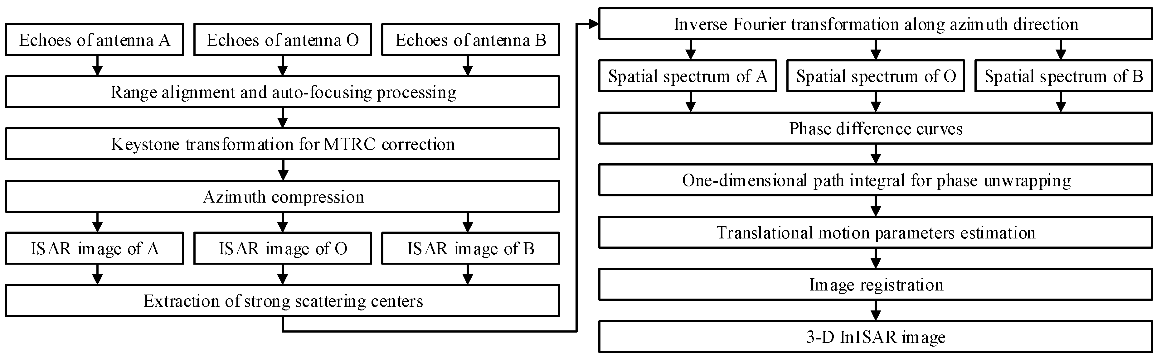
3. The Strong Scattering Centers Fusion (SSCF) Technique

In this subsection, the proposed SSCF technique is described in detail. This method can settle problems such as the “angle glint”, sensitivity to noise, and phase wrapping in motion parameter estimation.
The details of the proposed SSCF technique are described as follows.
Step 1) After data preprocessing (i.e., range alignment, autofocus [34,35], and MTRC correction), the spatial spectrums of radar echoes are obtained as s O ( m , k ) , s A ( m , k ) , and s B ( m , k ) , 1 m M and 1 k N , where M and N denote the number of samples and the number of pulses, respectively. Then, the ISAR images can be obtained as s O ( m , n ) , s A ( m , n ) , and s B ( m , n ) after azimuth compression, where 1 n N .
Step 2) Based on a fixed threshold, strong scattering areas on the object can be extracted from the three ISAR images. Firstly, the strongest scattering center in the first strong scattering area of antenna O can be easily found. Subsequently, the corresponding scattering centers in ISAR images of antenna A and antenna B can be confirmed, since they are distributed in the same range cell. This scattering center is then extracted in the image domain with a rectangular filter, whose length is determined by the main lobe width (3 dB) of the extracted scattering center. The noise is filtered in this step. This process is iterated to search for the localized strongest scattering center in all the strong scattering areas until the strongest scattering center in the last strong scattering area has been extracted.
Step 3) The extracted data of all SSCs in the image domain are rearranged to form new image matrices s O ( m , n ) , s A ( m , n ) , and s B ( m , n ) , where 1 m M , and M denotes the number of SSCs. By performing an inverse Fourier transformation on variable n , the new spatial spectrums are obtained as s O ( m , k ) , s A ( m , k ) , and s B ( m , k ) , respectively. Here, each row of the spatial spectrums contains information of only one scattering center. The phase difference curves s O * ( m , k ) s A ( m , k ) and s O * ( m , k ) s B ( m , k ) can be calculated as
φ x m ( k ) = 2 π λ L 1 2 2 L 1 ( x m + V x m k Δ t ) 2 y 0 ,
φ z m ( k ) = 2 π λ L 2 2 2 L 2 ( z m + V z m k Δ t ) 2 y 0 ,
where Δ t is the pulse repetition interval, and V x m and V z m are the estimated translation velocity of the m th strong scattering center.
Step 4) In the THz band, the wavelength is very short. On the other hand, in order to guarantee the precision of altitude measurement, a relative long baseline is required [7]. Therefore, the values of φ x m ( k ) and φ z m ( k ) usually exceed the range [ π , π ] , and the phase unwrapping operation is necessary. Here, the one-dimensional path integral method is adapted to achieve phase unwrapping of the motion measurement curves, and the theory is
Δ φ ( k ) = { φ ( k + 1 ) φ ( k ) | φ ( k + 1 ) φ ( k ) | π φ ( k + 1 ) φ ( k ) + 2 π φ ( k + 1 ) φ ( k ) < π φ ( k + 1 ) φ ( k ) 2 π φ ( k + 1 ) φ ( k ) > π φ new ( k + 1 ) = φ new ( k ) + Δ φ ( k ) ,
where φ ( k ) and φ new ( k ) are phases before and after phase unwrapping, respectively.
Step 5) The motion measurement curves along the x axis and z axis are calculated as
R x m ( k ) = φ x m new ( k ) λ y 0 2 π L 1 + L 1 2 = x m + V x m k Δ t ,
R z m ( k ) = φ z m new ( k ) λ y 0 2 π L 2 + L 2 2 = z m + V z m k Δ t .
The estimated velocities of each SSC can be obtained by fitting these time-dependent curves. Finally, the estimation values of translational motion parameters are acquired by intensity-weighted fusion of all SSCs:
V x = m = 1 M V x m A m m = 1 M A m ,    V z = m = 1 M V z m A m m = 1 M A m ;
where A m is the mean scattering intensity of the m th SSC in the ISAR images.
By compensating the radar echoes of antenna A and antenna B with the estimated motion parameters, the coordinates of the target are finally obtained from s O * ( y , f a ) s A ( y , f a ) and s O * ( y , f a ) s B ( y , f a ) ,
x P = λ y 0 2 π L 1 φ 1 + L 1 2 ,    z P = λ y 0 2 π L 2 φ 2 + L 2 2 .
The derivation of the value of y P is omitted here, as it can be directly obtained from the range scale in the ISAR images. To summarize the above analysis, a block scheme of the InISAR imaging procedure based on the SSCF technique is presented in Figure 2.
Regarding the InISAR imaging theory, the Doppler shift between ISAR images should be less than one-eighth of the Doppler cell after image registration to guarantee a relatively high InISAR imaging precision. Thus, the velocity estimation error Δ V should satisfy
| Δ V | < y 0 λ 8 L T a .
Equation (22) is applied as the criteria to evaluate the performance of the SSCF technique in this paper.

4. Results and Analysis

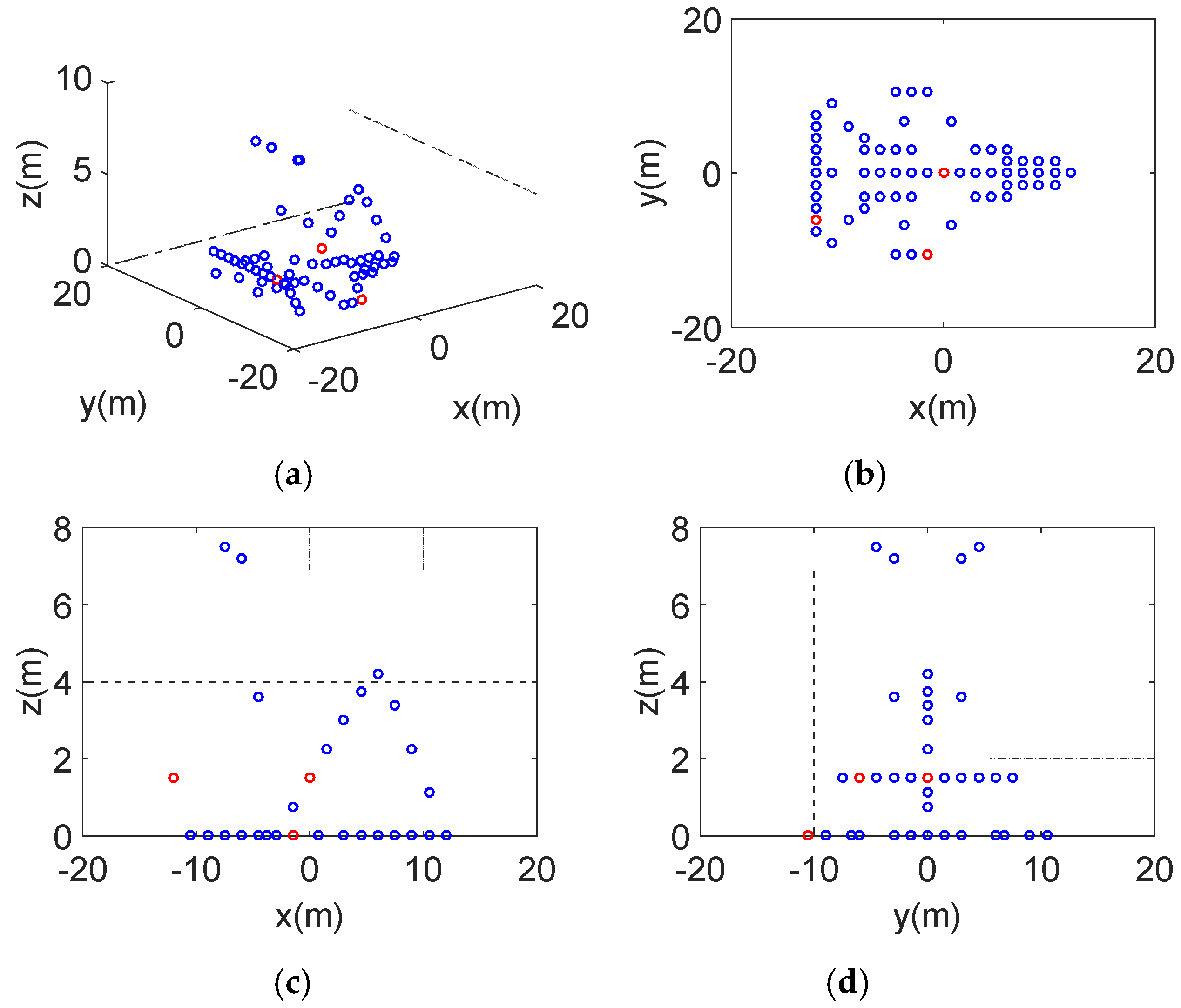
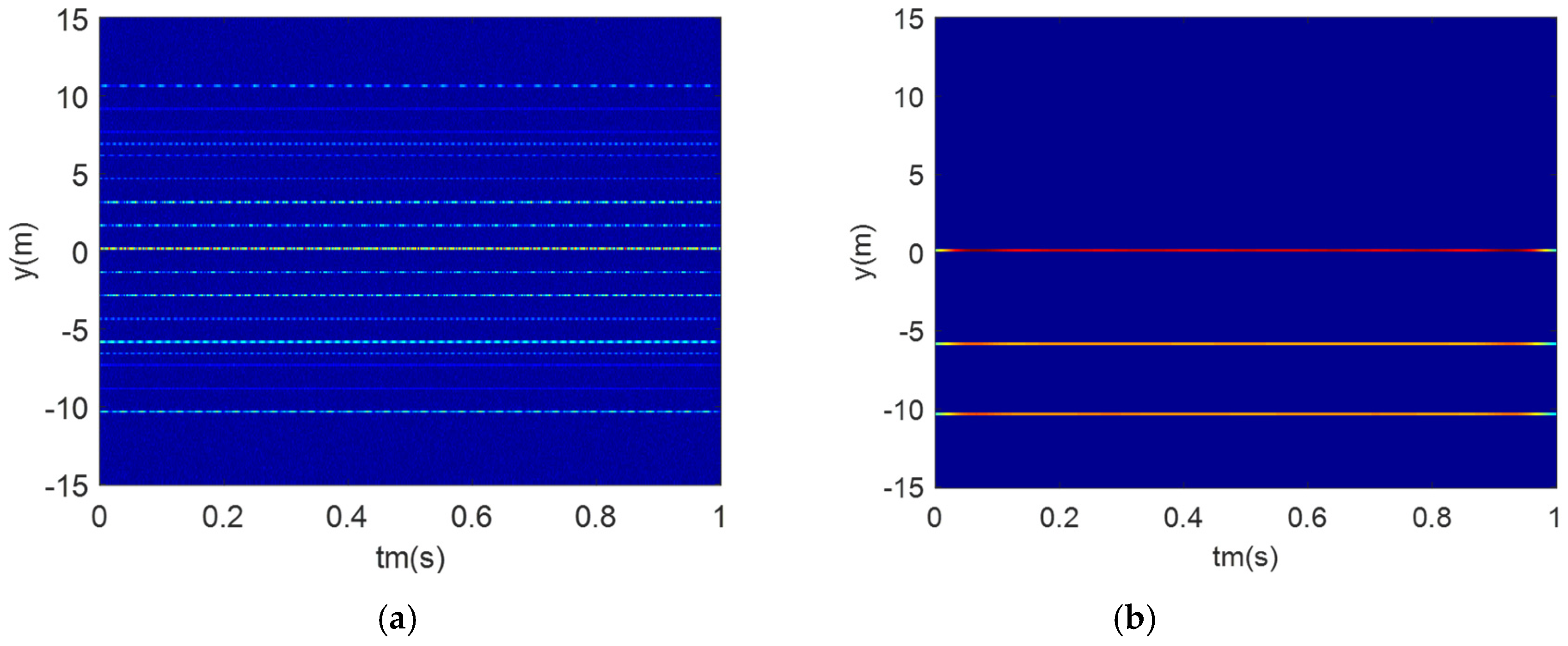
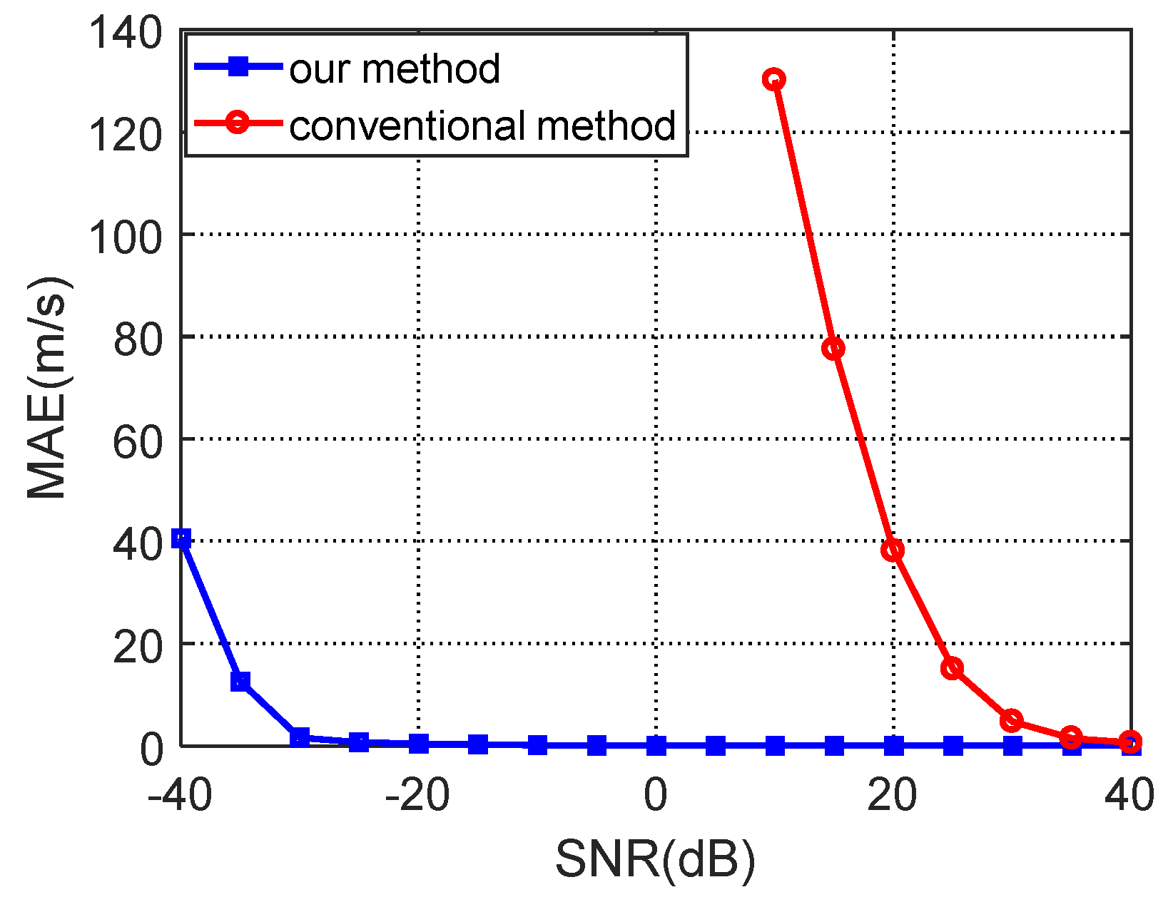
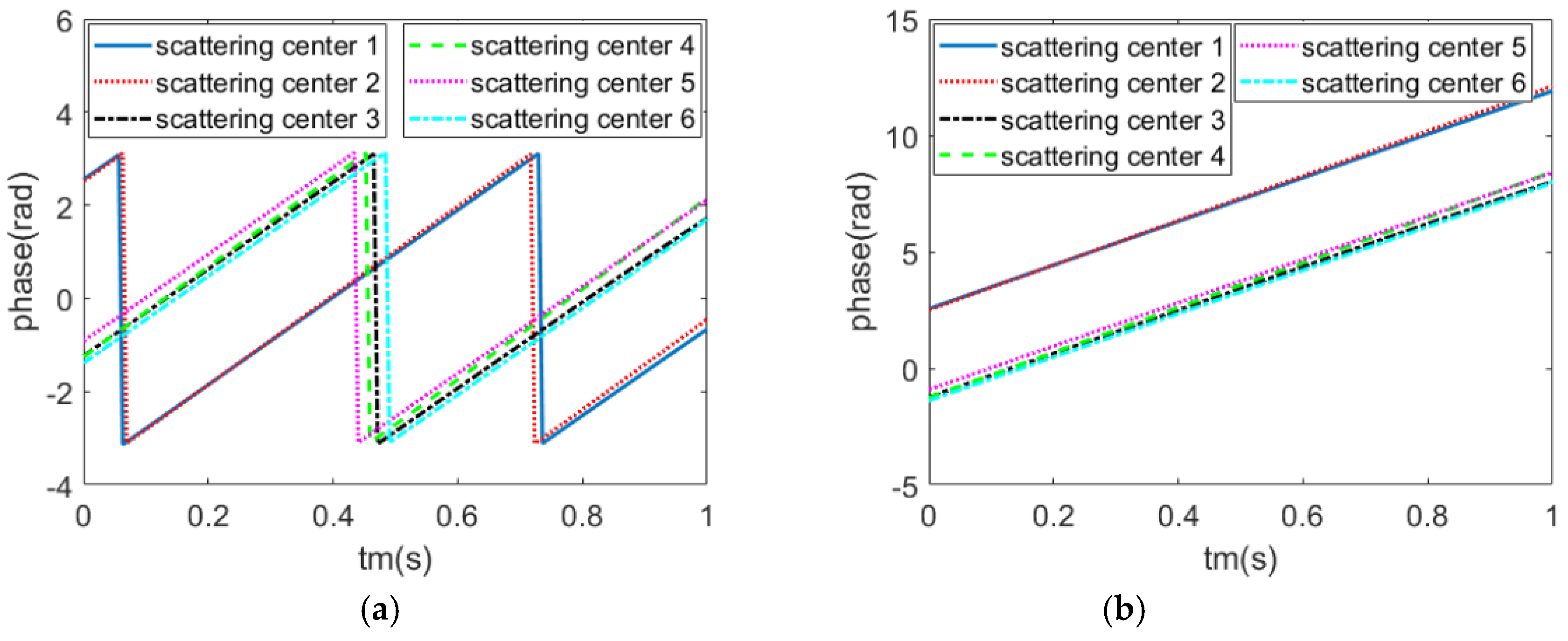
4.1. The Point Target Simulation Results

In order to verify the effectiveness of the proposed SSCF technique, an InISAR imaging simulation of a moving airplane model is presented. The parameters in the simulation are shown in Table 1. The airplane model contained 64 scattering centers, and the size of the airplane model was 21, 24, and 7.5 m in length, width, and height, respectively. For a vivid visualization, the model was depicted in four different views from four visual angles in Figure 3, with (a), (b), (c), and (d) corresponding to the 3-D view and projections on the xoy, xoz, and yoz planes, respectively. Three SSCs were assigned at the tail, wing, and fuselage, respectively, as highlighted with red circles in Figure 3. The ratio of scattering intensity between these SSCs and the others was 3:1. As a result, several ordinary scattering centers were distributed in the same range cell with the SSCs. The target was assigned to move at a constant velocity along the x direction, which led to image misregistration between ISAR images of antenna O and antenna A.
After range alignment, autofocus, and MTRC correction processing, three ISAR images were obtained. Based on the system parameters in Table 1, we calculated the Doppler shift between ISAR images of antenna A and antenna O at 5.5 cells. The range profiles of ISAR images at y = 0 of antenna A and antenna O are shown in Figure 4. It was obvious that there was a Doppler shift of six cells on the peak positions. To compare performances between the conventional method in [7] and our method, we added a pair of antennas with 0.04 m length of baseline to the conventional method because it used short baselines to achieve phase unwrapping of motion measurement curves.
Figure 5 shows the spatial spectrums of radar echoes, and Figure 6 shows the phase difference curves of the spatial spectrums, both with (a) corresponding to the conventional method and (b) corresponding to our method. The SNR was 0 dB in this simulation. It can be seen from Figure 5a that the multiple scattering centers in a fixed range cell introduced a serious “angle glint” phenomenon. The “angle glint” phenomenon was eliminated by extracting the SSCs, as shown in Figure 5b. The influence of the multiscattering centers in motion parameter estimations is visualized in Figure 6a. Firstly, the “angle glint” phenomenon and noise introduced serious nonlinearity to the phase difference curves, which destroyed the real phase difference relationship and deteriorated the estimation precision of motion parameters. Secondly, without the short baseline, different scattering centers had different phase wrapping positions, and the one-dimensional path integral method was not applicable in this condition. In contrast, the curves in Figure 6b were linear, and the phase wrapping positions of each curve were constant. Noise was effectively filtered with the filter operation in the image domain, which ensured an excellent linearity of the motion trajectory even under a low SNR.
Based on the one-dimensional path integral method, the phase difference curves of the three SSCs after phase unwrapping were acquired, as shown in Figure 7. All curves were absolutely linear with no fluctuation. Subsequently, translational motion parameters were easily estimated based on polynomial curve fitting and intensity-weighted fusion operation. In this simulation, the estimated velocities of the conventional method and our method were 68.678 and 300.057 m/s, respectively, which meant the conventional method was invalid under this low-SNR simulation environment. The estimated velocity of our method was nearly the same as the real velocity, which verified the effectiveness of the proposed SSCF technique. By compensating the estimated velocity of our method to the echo signals of antenna A, the final imaging results are shown in Figure 8, with (a) corresponding to the range profiles at y = 0 of antenna A and antenna O and (b) corresponding to the final InISAR imaging results. It can be seen from Figure 8a that the Doppler shift was eliminated, and image registration was achieved. In Figure 8b, the red circles are the real positions of the target, and the blue dots are the InISAR imaging results. It was clear that the InISAR image and the target model were precisely overlapped.
At the end of this simulation, the antinoise abilities of the two methods were evaluated. With our simulation parameters, the maximum allowed mean absolute error (MAE) of the estimated velocity in this simulation was derived as 6.8 m/s on the basis of Equation (22). The MAE of the estimated velocity is defined as
MAE = i = 1 N | V i V | / N ,
where V i is the ith estimated velocity, V is the real velocity, and N is the number of simulation times. Here, the MAE of the estimated velocity was provided based on 100 Monte Carlo simulations under different SNR environments, as shown in Figure 9. The MAE of the conventional method was larger than 6.8 m/s when the SNR was under 30 dB, which meant the antinoise performance of the conventional method was very poor. This method was only suitable for extremely high SNR environments. The MAE of our method was under 6.8 m/s when the SNR was larger than −30 dB. The low MEA in estimated velocity proved the excellent antinoise ability of the proposed SSCF technique.
In order to show the superiority of the proposed SSCF technique over the past methods, performance comparisons of the frequency domain searching (FDS) method in [4], respective reference distance compensation (RRDC) method in [5] and [6], angular motion parameters estimation (AMPE) method in [7], and proposed SSCF technique in this paper are listed in Table 2. The algorithm reconstruction times (excluding the echo generation process) were obtained on a desktop computer with Intel core i7-7820X 3.60GHz CPU and 32GB RAM using Matlab codes. The reconstruction time of the FDS method depended on the initial value and searching step of motion parameters. In this experiment, the initial value and searching step were set as 200 and 3 m/s, respectively, and a typical single-parameter optimization algorithm was adapted. From Table 2, it was seen that the FDS method was too time-consuming to fulfill the requirement of real time imaging. The RRDC method had the fastest imaging speed, but the radar needed to have ranging function. Besides, it was highly challenging to acquire accurate distances from the reference center to the other receivers (except the one as both a transmitter and receiver). The AMPE method needed a complex system structure, and the antinoise ability was poor. The SSCF technique proposed in this paper was advantageous in its high computing efficiency, excellent antinoise performance, and simple system structure. Therefore, the SSCF technique was more suitable for image registration in InISAR imaging.

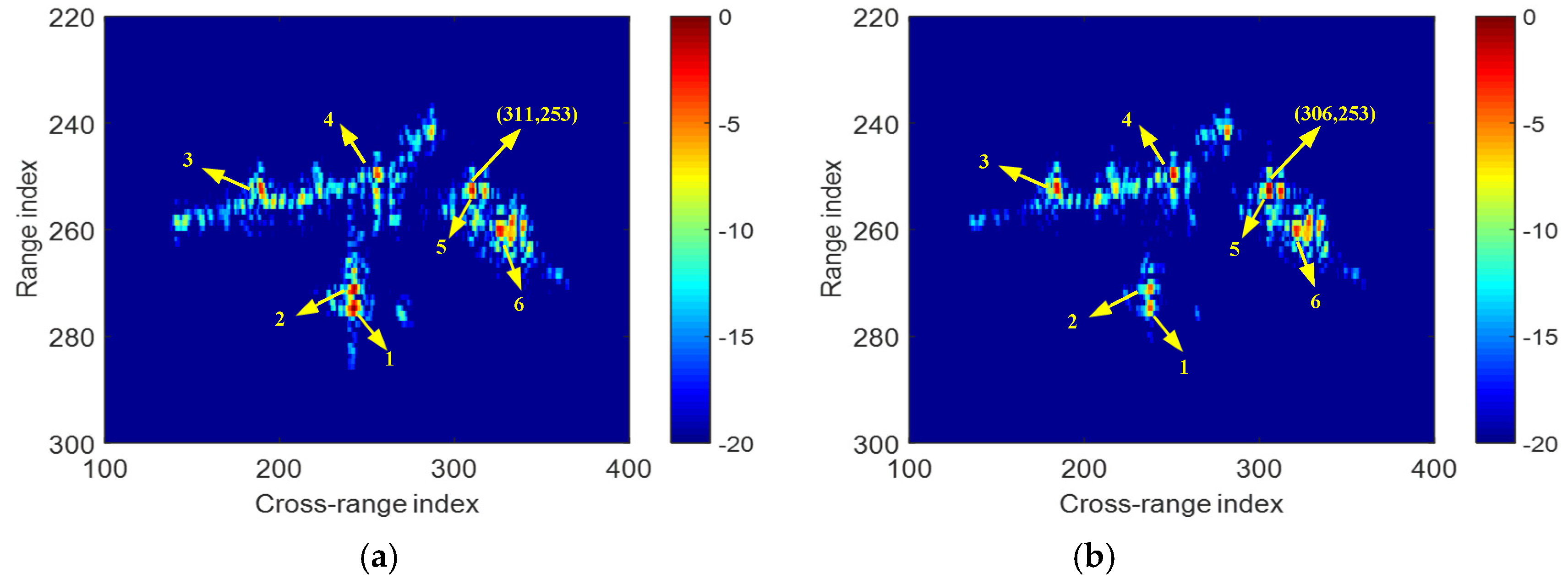
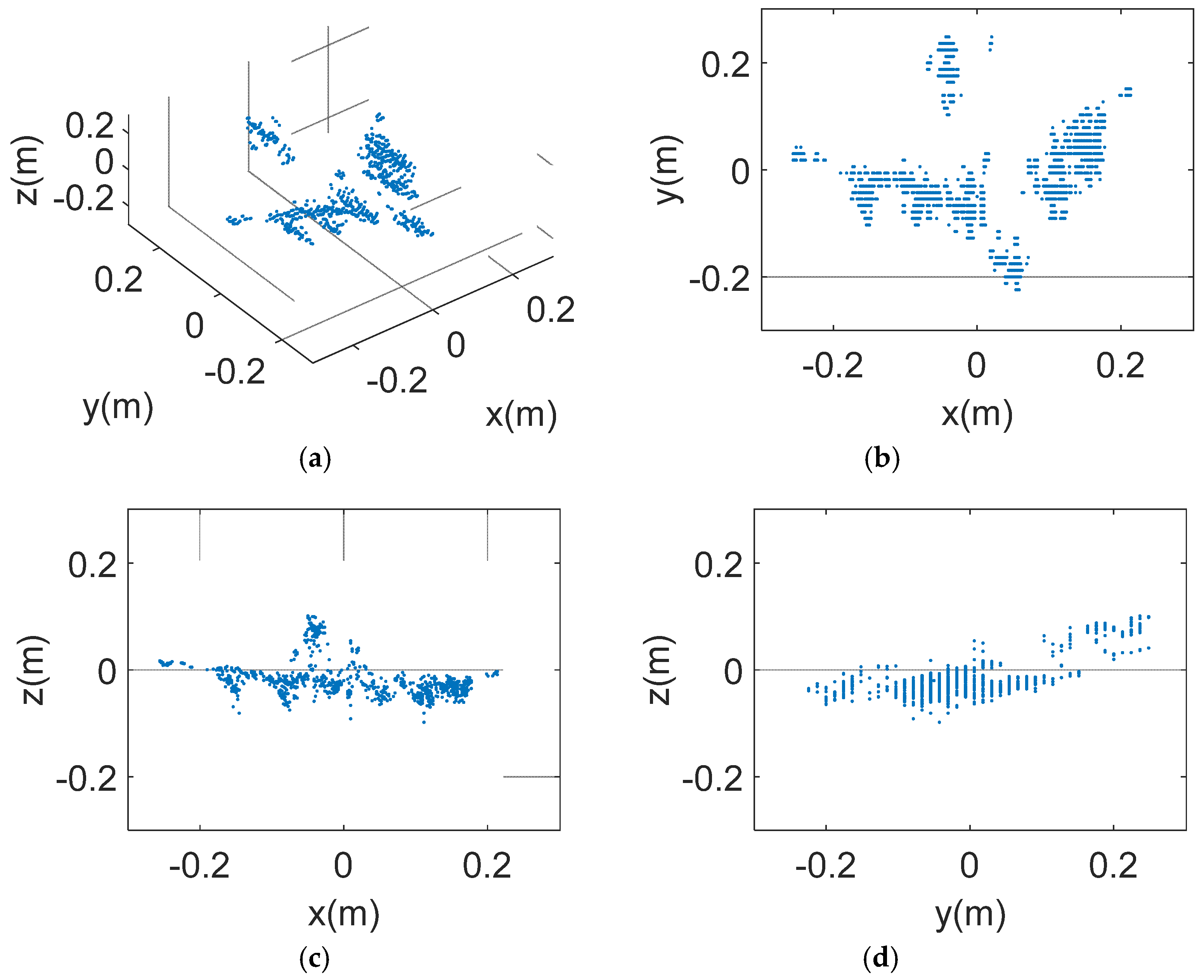
4.2. Experimental Results

In order to further verify the effectiveness of the proposed SSCF technique, equivalent verification experiments in the laboratory environment were carried out. The schematic diagram of the THz radar system and the photograph of the front-end setup is shown in Figure 10. The five antennas were arranged in two rows, with three receiving antennas in the upper row and one transmitting antenna and one receiving antenna in the other row. R1 and R2 formed the vertical interferometric baseline, and R2 and R3 formed the horizontal interferometric baseline. Both the vertical and horizontal baseline lengths were 2.1 cm. R4 was ignored in the InISAR experiment. Besides InISAR imaging, this system also had many other potential applications such as InSAR imaging, ViSAR imaging, and micromotion target 3-D imaging. The THz radar system was based on the linear frequency modulated pulse principle. A chirped signal ranging from 217.1 to 222.1 GHz was transmitted, and the echo signals were received by the four receiving antennas.
The experimental configuration is shown in Figure 11. In the experiment, the THz radar was put on a one-dimensional horizontal guide platform, and the velocity of radar was 1 m/s. The vertical distance between the radar and the target was 10 m, and the initial connection from the target to the radar platform was perpendicular to the motion direction. This was a typical SAR imaging scenario, but it was equivalent in that the radar was static, and the target moved along the horizontal direction, which matched the InISAR scenario described in this paper. To decrease the SNR of the radar echoes, the power transmitted from the radar was reduced to 10 mW. The pulse width was 163.8 μs, the pulse repetition frequency was 2500 Hz, the sampling frequency was 12.5 MHz, and the data acquisition time was 1 s. The target was an Airbus A380 model. The length, wingspan, and height of the model were 45, 52, and 17 cm, respectively.
The reflected signals received by R1, R2, and R3 were used to form the InISAR images, and the reference signal was the reflected signal of a corn reflector located at the same position of the airplane model received by R2. Thus, the imaging geometry is the same as the discussed L-shaped three-antenna configuration. During the imaging process, nonlinearity of the signal frequency and the inconsistencies of the amplitudes and phases among channels were compensated together with the reference signal, and a phase gradient autofocus algorithm [36] was adopted to compensate the influence of guide platform vibration. The ISAR images of channels R2 and R3 were interpolated three times and shown in Figure 12. Taking the strong scattering center at the right wing as an example, there are five Doppler cells that deviated along the azimuth direction.
Based on a threshold of 3 dB, the ISAR image of six SSCs were extracted, as indicated in Figure 12. The spatial spectrums of these SSCs were then acquired. The phase difference curves of spatial spectrums between channel R2 and R3 are shown in Figure 13, with (a) and (b) corresponding to the conditions before and after phase unwrapping processing, respectively. As illustrated in Figure 13a, all curves were linear, and the phase wrapping position of each curve was constant. With our experimental parameters, the maximum allowed error in velocity estimation for precise image registration was 0.0812 m/s on the basis of Equation (22). Based on the motion measurement curves in Figure 13b, velocity along the horizontal direction was estimated as 0.9737 m/s, which satisfied the estimated precision of parameters for image registration. After compensating the velocity to the echo signal of channel R3, image registration was achieved. Finally, the InISAR imaging results were obtained, as shown in Figure 14, with (a), (b), (c), and (d) corresponding to the 3-D view and projections on the xoy, xoz, and yoz planes, respectively. From the InISAR imaging results, we saw that the key parts in the A380 model such as the engine, wing, and vertical fin could be clearly identified, and the imaging results were clear and close to the real airplane model. These results further verified the effectiveness of the proposed SSCF method. In this chapter, we did not compare the performance between our method and the conventional method because the baseline length in this equivalent verification experiment could not be any shorter. Phase wrapping in the motion measurement curves was inevitable. In this condition, the conventional method was not applicable.

5. Discussion

Taking the algorithm’s efficiency, practicability, robustness, and precision into consideration, the simulation and experimental results have verified that the SSCF technique proposed in this paper is the most suitable method for image registration in THz InISAR imaging. Until now, there has been limited research on InISAR imaging with terahertz radars. This paper takes the lead in putting forward a THz InISAR imaging system, and it has carried out InISAR experiments in the laboratory environment. In the next stage, long-distance experiments that connect a traveling-wave tube amplifier will be carried out to verify the SSCF technique proposed in this paper.

6. Conclusions

In this paper, a translational motion parameter estimation method based on SSCF technique was proposed to achieve image registration in InISAR imaging under a low-SNR environment. The “angle glint” phenomenon and phase wrapping in motion measurement curves were solved, and the interference of noise was also removed with the rectangular filter operation in image domain. Based on this method, the estimation accuracy of translational motion parameters can fulfill image registration requirements when the SNR was larger than −30 dB. Both simulation and experimental results are presented to verify the validity of the proposed method. The method also can be extended to target with a more complicated motion feature. Until now, the experiments were carried out in a laboratory environment, but the work in this paper can provide support to the remote application of THz InISAR imaging systems in the future.

Author Contributions

Y.Z. was responsible for the theoretical work and performed the experiments. Y.Q. and H.W. provided the experimental environment and equipment. B.D. and Q.Y. revised the paper. The authors also wish to extend their sincere thanks to editors and reviewers for their careful reading and fruitful suggestions.

Funding

This work was supported by the National Nature Science Foundation of China (Grant No. 61871386).

Conflicts of Interest

The authors declare no conflict of interest.

References

  1. Xu, X.; Narayanan, R.M. Three-dimensional interferometric ISAR imaging for target scattering diagnosis and modeling. IEEE Trans. Image Process. 2001, 10, 1094–1102. [Google Scholar]
  2. Wang, G.; Xia, X.; Chen, V.C. Three-dimensional ISAR imaging of maneuvering targets using three receivers. IEEE Trans. Image Process. 2001, 10, 436–447. [Google Scholar] [CrossRef] [PubMed]
  3. Given, J.A.; Schmidt, W.R. Generalized ISAR—Part II: Interferometric techniques for three-dimensional location of scatterers. IEEE Trans. Image Process. 2005, 14, 1792–1797. [Google Scholar] [CrossRef]
  4. Biao, T.; Na, L.; Yang, L. A Novel image registration method for InISAR imaging system. SPIE Secur. Def. 2014, 9252. [Google Scholar] [CrossRef]
  5. Liu, C.; He, F.; Gao, X. Novel reference range selection method in InISAR imaging. J. Syst. Eng. Electron. 2012, 23, 512–521. [Google Scholar] [CrossRef]
  6. Tian, B.; Shi, S.; Liu, Y. Image registration of interferometric inverse synthetic aperture radar imaging system based on joint respective window sampling and modified motion compensation. J. Appl. Remote Sens. 2015, 9, 095097. [Google Scholar] [CrossRef]
  7. Zhang, Q.; Yeo, T.S.; Du, G. Estimation of three-dimensional motion parameters in interferometric ISAR imaging. IEEE Trans. Geosci. Remote Sens. 2004, 42, 292–300. [Google Scholar] [CrossRef]
  8. Felguera-Martin, D.; Gonzalez-Partida, J.T.; Almorox-Gonzalez, P. Interferometric inverse synthetic aperture radar experiment using an interferometric linear frequency modulated continuous wave millimeter-wave radar. IET Radar Sonar Navig. 2011, 5, 39–47. [Google Scholar] [CrossRef]
  9. Ng, W.H.; Tran, H.T.; Martorella, M. Estimation of the total rotational velocity of a non-cooperative target with a high cross-range resolution three-dimensional interferometric inverse synthetic aperture radar system. IET Radar Sonar Navig. 2017, 11, 1020–1029. [Google Scholar] [CrossRef]
  10. Xu, G.; Xing, M.; Xia, X.G. 3D geometry and motion estimations of maneuvering targets for interferometric ISAR with sparse aperture. IEEE Trans. Image Process. 2016, 25, 2005–2020. [Google Scholar] [CrossRef]
  11. Martorella, M.; Stagliano, D.; Salvetti, F. 3D interferometric ISAR imaging of non-cooperative targets. IEEE Trans. Aerosp. Electron. Syst. 2014, 50, 3102–3114. [Google Scholar] [CrossRef]
  12. Dengler, R.J.; Cooper, K.B.; Chattopadhyay, G. 600 GHz Imaging Radar with 2 cm Range Resolution. In Proceedings of the IEEE/MTT-S International Microwave Symposium, Honolulu, HI, USA, 3–8 June 2007; pp. 1371–1374. [Google Scholar]
  13. Cooper, K.B.; Dengler, R.J.; Chattopadhyay, G. A high-resolution imaging radar at 580 GHz. IEEE Microw. Wirel. Compon. Lett. 2008, 18, 64–66. [Google Scholar] [CrossRef]
  14. Cooper, K.B.; Dengler, R.J.; Llombart, N. Penetrating 3-D imaging at 4 and 25 meter range using a submillimeter-wave radar. IEEE Trans. Microw. Theory Tech. 2008, 56, 2771–2778. [Google Scholar] [CrossRef]
  15. Llombart, N.; Cooper, K.B.; Dengler, R.J. Time-delay multiplexing of two beams in a terahertz imaging radar. IEEE Trans. Microw. Theory Tech. 2010, 58, 1999–2007. [Google Scholar] [CrossRef]
  16. Cooper, K.B.; Dengler, R.J.; Llombart, N. THz imaging radar for standoff personnel screening. IEEE Trans. Terahertz Sci. Technol. 2011, 1, 169–182. [Google Scholar] [CrossRef]
  17. Blazquez, B.; Cooper, K.B.; Llombart, N. Time-delay multiplexing with linear arrays of THz radar transceivers. IEEE Trans. Terahertz Sci. Technol. 2014, 4, 232–239. [Google Scholar] [CrossRef]
  18. Sheen, D.M.; Mcmakin, D.L.; Thomas, E.H. Active Millimeter-Wave Standoff and Portal Imaging Techniques for Personnel Screening. In Proceedings of the IEEE Conference on Technologies for Homeland Security, Waltham, MA, USA, 11–12 May 2009. [Google Scholar]
  19. Sheen, D.M.; Hall, T.E.; Severtsen, R.H. Active wideband 350 GHz imaging system for concealed-weapon detection. Proc. SPIE 2009, 7309. [Google Scholar] [CrossRef]
  20. Gao, X.; Li, C.; Gu, S. Design, Analysis and Measurement of a Millimeter Wave Antenna Suitable for Stand off Imaging at Checkpoints. J. Infrared Millim. Terahertz Waves 2011, 32, 1314–1327. [Google Scholar] [CrossRef]
  21. Gu, S.; Li, C.; Gao, X. Terahertz aperture synthesized imaging with fan-beam scanning for personnel screening. IEEE Trans. Microw. Theory Tech. 2012, 60, 3877–3885. [Google Scholar] [CrossRef]
  22. Sun, Z.; Li, C.; Gu, S. Fast Three-Dimensional Image Reconstruction of Targets Under the Illumination of Terahertz Gaussian Beams with Enhanced Phase-Shift Migration to Improve Computation Efficiency. IEEE Trans. Terahertz Sci. Technol. 2014, 4, 479–489. [Google Scholar] [CrossRef]
  23. Cheng, B.B.; Cui, Z.M.; Lu, B. 340 GHz 3-D imaging radar with 4Tx-16Rx MIMO array. IEEE Trans. Terahertz Sci. Technol. 2018, 5, 509–519. [Google Scholar] [CrossRef]
  24. Gao, J.; Cui, Z.M.; Cheng, B.B. Fast Three-Dimensional Image Reconstruction of a Standoff Screening System in the Terahertz Regime. IEEE Trans. Terahertz Sci. Technol. 2018, 4, 38–51. [Google Scholar] [CrossRef]
  25. Essen, H.; Wahlen, A.; Sommer, R. High-Bandwidth 220 GHz Experimental Radar. Electron. Lett. 2007, 43, 1114–1116. [Google Scholar] [CrossRef]
  26. Stanko, S.; Caris, M.; Wahlen, A. Millimeter Resolution with Radar at Lower Terahertz. In Proceedings of the IEEE International Radar Symposium, Dresden, Germany, 19–21 June 2013; pp. 235–238. [Google Scholar]
  27. Caris, M.; Stanko, S.; Palm, S. 300 GHz radar for high resolution SAR and ISAR applications. In Proceedings of the 16th International Radar Symposium, Dresden, Germany, 24–26 June 2015; pp. 577–580. [Google Scholar]
  28. Kim, S.; Fan, R.; Dominski, F. A 235 GHz Radar for Airborne Applications. In Proceedings of the 2018 IEEE Radar Conference, Oklahoma City, USA, 23–27 April 2018; pp. 1549–1554. [Google Scholar]
  29. Cheng, B.B.; Jiang, G.; Wang, C. Real-time imaging with a 140 GHz inverse synthetic aperture radar. IEEE Trans. Terahertz Sci. Technol. 2013, 3, 594–605. [Google Scholar] [CrossRef]
  30. Ding, J.; Kahl, M.; Loffeld, O. THz 3-D image formation using SAR techniques: Simulation, processing and experimental results. IEEE Trans. Terahertz Sci. Technol. 2013, 3, 606–616. [Google Scholar] [CrossRef]
  31. Danylov, A.A.; Goyette, T.M.; Waldman, J. Terahertz Inverse Synthetic Aperture Radar (ISAR) Imaging with a Quantum Cascade Laser Transmitter. Opt. Express 2010, 18, 16264–16272. [Google Scholar] [CrossRef]
  32. Zhang, B.; Pi, Y.; Li, J. Terahertz Imaging Radar with Inverse Aperture Synthesis Techniques: System Structure, Signal Processing, and Experiment Results. IEEE Sens. J. 2015, 15, 290–299. [Google Scholar] [CrossRef]
  33. Yang, Q.; Qin, Y.L.; Zhang, K. Experimental research on vehicle-borne SAR imaging with THz radar. Microw. Opt. Technol. Lett. 2017, 59, 2048–2052. [Google Scholar] [CrossRef]
  34. Ye, W.; Yeo, T.S.; Bao, Z. Weighted least square estimation of phase errors for SAR/ISAR autofocus. IEEE Trans. Geosci. Remote Sens. 1999, 37, 2487–2494. [Google Scholar] [CrossRef]
  35. Cao, P.; Xing, M.; Sun, G. Minimum Entropy via Subspace for ISAR Autofocus. IEEE Geosci. Remote Sens. Lett. 2010, 7, 205–209. [Google Scholar] [CrossRef]
  36. Wahl, D.E.; Eichel, P.H.; Ghiglia, D.C. Phase gradient autofocus—A robust tool for high resolution SAR phase correction. IEEE Trans. Aerosp. Electron. Syst. 1994, 30, 827–835. [Google Scholar] [CrossRef]
Figure 1. Schematic of the three-receiver interferometric inverse synthetic aperture radar (InISAR) imaging configuration.
Remotesensing 11 01221 g001
Figure 2. The flowchart of InISAR imaging based on the strong scattering centers fusion (SSCF) technique.
Remotesensing 11 01221 g002
Figure 3. Four different views of the airplane model. (a) 3-D view; (b) xoy view projection; (c) xoz view projection; and (d) yoz view projection.
Remotesensing 11 01221 g003
Figure 4. ISAR images at y = 0 of antenna O and antenna A before image registration.
Remotesensing 11 01221 g004
Figure 5. The spatial spectrums of radar echoes. (a) Conventional method. (b) Our method.
Remotesensing 11 01221 g005
Figure 6. Phase difference curves of spatial spectrums. (a) Conventional method. (b) Our method.
Remotesensing 11 01221 g006
Figure 7. Phase difference curves after phase unwrapping based on the SSCF technique.
Remotesensing 11 01221 g007
Figure 8. Imaging results after image registration. (a) ISAR images at y = 0 of antenna O and antenna A. (b) InISAR imaging results.
Remotesensing 11 01221 g008
Figure 9. The mean absolute error (MAE) under different signal-to-noise ratio.
Remotesensing 11 01221 g009
Figure 10. The terahertz radar system. (a) Schematic diagram. (b) Photograph of the front-end setup.
Remotesensing 11 01221 g010
Figure 11. The experimental configuration.
Remotesensing 11 01221 g011
Figure 12. The ISAR images of A380 model. (a) Channel R2. (b) Channel R3.
Remotesensing 11 01221 g012
Figure 13. Phase difference curves of the spatial spectrum. (a) Before phase unwrapping. (b) After phase unwrapping.
Remotesensing 11 01221 g013
Figure 14. InISAR imaging results of the airplane model. (a) 3-D view; (b) xoy view projection; (c) xoz view projection; and (d) yoz view projection.
Remotesensing 11 01221 g014
Table 1. Parameter settings of the radar system and target.
ParameterSetting Value
Carrier frequency220 GHz
Bandwidth5 GHz
Pulse width 50 us
Pulse repetition frequency1000 Hz
Pulse number1000
Sampling frequency20 MHz
Target speed(300, 0, and 0 m/s)
Antenna O location(0, 20,000, and 0 m)
Antenna A location(0.5, 20,000, and 0 m)
Antenna B location(0, 20,000, and 0.5 m)
Table 2. Comparison of algorithm performances.
MethodReconstruction TimeNumber of ChannelsAnti-Noise AbilityNeed Ranging Function
Frequency domain Searching (FDS)23.145 s3StrongNo
Respective Reference Distance Compensation (RRDC)0.699 s3StrongYes
Angular Motion Parameters Estimation (AMPE)0.744 s9WeakNo
Strong Scattering Centers Fusion (SSCF)1.657 s3StrongNo

