Article

Modeling the Stereoscopic Features of Mountainous Forest Landscapes for the Extraction of Forest Heights from Stereo Imagery

1
State Key Laboratory of Remote Sensing Science, Institute of Remote Sensing and Digital Earth, Chinese Academy of Sciences, Beijing 100101, China
2
Department of Geographical Sciences, University of Maryland, College Park, MD 20740 USA
*
Author to whom correspondence should be addressed.
Remote Sens. 2019, 11(10), 1222; https://doi.org/10.3390/rs11101222
Submission received: 28 March 2019 / Revised: 12 May 2019 / Accepted: 20 May 2019 / Published: 23 May 2019
(This article belongs to the Section Forest Remote Sensing)

Abstract

:
Spaceborne stereoscopic systems have been growing in recent years, and the point cloud extracted from spaceborne stereo imagery has been used to measure forest spatial structures. These systems work on different viewing angles and image spatial resolutions, which are two critical factors determining the quality of the derived point cloud. In addition, the complex terrain is also a great challenge for the regional mapping of forest spatial structures using spaceborne stereo imagery. Although several theoretical models for simulating multi-view spectral features of forest canopies have been developed, there is hardly any report of a stereoscopic analysis using these models due to the limited size of the simulated forest scenes and the lack of a geometric sensory model (i.e., physical relationship between two-dimensional image coordinates and three-dimensional georeferenced coordinates). The stereoscopic features (i.e., parallax) are, as important as the spectral features contained in the multi-view images of a targeted area, the basis for the extraction of a point cloud. In this study, a new model, referred to as LandStereo model, has been proposed, which is capable of simulating the stereoscopic features of forest canopies over mountainous areas at landscape scales. The model comprised five parts, including defining the mountainous forest landscapes, setting the sun-senor observation geometry, simulating images, generating ground control points, and building geometric sensor models. The LandStereo model was validated over three different scenes, including flat forest landscapes, bare mountain landscapes, and mountainous forest landscapes. The results clearly demonstrated that the LandStereo model worked well on simulating stereoscopic features of both terrains and forest canopies at landscape scales. The extracted height of a forest canopy top from simulated stereo imagery was highly correlated to the truth (R2 = 0.96 and RMSE = 0.99 m) over the flat terrains and (R2 = 0.92 and RMSE = 1.15 m) over the mountainous areas. The LandStereo model provided a powerful tool to further our understanding of the relationships between forest spatial structures and point cloud extracted from stereo imagery acquired from different view angles and spatial resolutions under complex terrain conditions.

Graphical Abstract

1. Introduction

The forest spatial structure is a key determinant of the forest ecosystem functions due to the height-structured competitions for light [1,2]. High spatial resolution maps of three-dimensional (3D) structures of forests are a necessary prerequisite to characterize the impact of human and natural forces on forest ecosystems, habitat, biodiversity, and climate change [3]. Several new space assets, which could directly measure the vertical structures of ground objects, are being prepared to meet this requirement. National Aeronautics and Space Administration (NASA) of the United States (US) deployed its Global Ecosystem Dynamics Investigation (GEDI) on the International Space Station (ISS) in 2018, which could provide billions of measurements of ground elevations and forest vertical structures in LiDAR footprints [4]. The European BIOMASS mission, which is planned to be launched around 2021, is one that is specifically designed for mapping global forest biomass using P-band polarimetric interferometry (Pol-InSAR) [5]. However, neither the GEDI nor the BIOMASS mission could provide global solutions. The coverage restriction of the BIOMASS mission over Europe, and North and Central America has been imposed by the US Department of Defense Space Objects Tracking Radar (SOTR) stations [6]. The GEDI could not provide wall-to-wall coverage as a result of its data acquisition strategy of point sampling. Gaps among its ground tracks and between adjacent swaths still remains [4]. Other sources of dataset should be used to fill the spatial gaps of both the BIOMASS mission and the GEDI.
Another dataset which could directly measure the vertical structures of ground objects, is stereo imagery. Spaceborne photogrammetric missions with a capability of global coverage have been in orbit, or, are under construction. The Advanced Spaceborne Thermal Emission and Reflection Radiometer (ASTER) began to make stereoscopic observations in 1999 [7]. The French SPOT series satellites started to acquire stereo imagery from SPOT-5 in 2002 [8]. The Japanese Panchromatic Remote-Sensing Instrument for Stereo Mapping (PRISM) onboard the Advanced Land Observing Satellite (ALOS) has collected global stereo imagery between 2006 and 2011 [9]. The successor of ALOS/PRISM, i.e., ALOS-3, is scheduled to be launched around 2020. China has also launched two civil stereoscopic satellites (ZY-3 01 and ZY-3 02) in 2012 and 2016, respectively. The third satellite, referred to as GaoFen-7 (GF-7), has a higher spatial resolution and will be deployed in 2019.
With the growing number of spaceborne photogrammetric missions and the rapid developments of automatic tools for stereoscopic data processing in recent years, researchers in the domain of remote sensing are gradually paying more attentions to the extraction of forest spatial structures using spaceborne stereo imagery. Ni et al. (2015) examined the forest heights contained in the ASTER stereoscopic observations [10]. St-Onge et al. (2008) mapped the forest height and aboveground biomass, using stereo image assisted by the digital terrain model (DTM) of LiDAR over Quebec, Canada [11]. Neigh et al. (2014) characterized the canopy height of forest stands, using stereo images, at three different locations, including the Harvard Forest in Central Massachusetts, Jamison in Central South Carolina and Hoquiam on the central west coast of Washington State [12]. Montesano et al. (2017) mapped the stereogrammetric height of the boreal forest using high resolution spaceborne imagery, acquired by Digital Globe’s Worldview-1, and Worldview-2 satellites [13]. Ni et al. (2014) analyzed the features of point clouds synthesized from multi-view ALOS/PRISM data [14].
The aforementioned studies have demonstrated that it was feasible to extract forest canopy heights from point clouds of the spaceborne stereoscopic imagery. However, the quality of the point cloud is largely determined by the observation geometry [13] and image resolutions, and could also be affected by cloud cover, topographic shadowing, and other factors affecting the light environment (diffuse versus direct lighting) [15]. The spaceborne photogrammetric missions work on different observation geometry and image resolutions. For example, the spatial resolution of the ASTER stereo imagery is 15 m, with a stereo angle (i.e., convergence angle) of 27.6° [16]; the spatial resolution of the SPOT-5 stereo image is 5 m × 10 m, with a stereo angle of 40° (two sensors both looking 20° off-nadir—one forward and one backward) [17]; the nominal nadir image resolution of ALOS/PRISM is 2.5 m with stereo angles of ±23.8° [18]; the spatial resolution of the ALOS-3 nadir image is designed as 0.8 m with stereo angles of 23.8° [19]. These missions are initiated in the field of surveying and mapping, for the mapping of global digital elevation models (DEM) [20], rather than for the extraction of forest canopy heights. In order to fully understand the impact of the various factors mentioned above on the quality of point cloud derived from stereo imagery, theoretical models are needed to systematically simulate stereoscopic images at different observation geometry and environmental conditions. Specifically, the simulated imagery can be used to explore the relationships between the spatial structures of different forest types and the point clouds from stereo imagery with different resolutions acquired by different observation geometry, under different environmental circumstances.
Some spaceborne photogrammetric missions are composed of three cameras pointing forward, nadir, and backward, such as the ALOS/PRISM and Chinese ZY-3, while others are fulfilled by constellations, such as the Pleiades-1 or by changing satellite attitudes, such as satellites of worldview series. The stereo images of one place are acquired by cameras viewing at different angles. Therefore, stereo images are, in fact, multi-view optical imagery. Several optical models of forest canopies have been developed over the past three decades, such as, the geometric–optical bidirectional reflectance model [21], four-scale bidirectional reflectance model [22], radiosity-graphics model [23], Geometric Optical-Radiative Transfer (GORT) model [24], Discrete Anisotropic Radiative Transfer (DART) model [25], Radiosity Applicable to Porous IndiviDual (RAPID) model [26], large-scale remote sensing data and image simulation framework [27], and so on. These models focused on the simulation of multi-view spectral features. There is hardly any report on the stereoscopic analysis of multi-view geometrical features of forest canopies simulated by these optical theoretical models. As the multispectral feature is commonly used in the remote sensing society to represent the reflection of incoming radiation from a target, in this paper, the stereoscopic feature is used to represent the parallax information contained in the images of a targeted area viewed from multiple directions.
In this study, we introduced a new model, referred to as a LandStereo model, based on an open-source freeware of ray-tracing, i.e., the Persistence of Vision Ray tracer (POV-Ray), which has been used for creating stunning graphics [28] and terrestrial stereo pairs [29]. The LandStereo model was developed to simulate the stereoscopic features of a forest at landscape scales (at least several kilometers by several kilometers) with the given observation geometry and image resolutions. The model consisted of five parts, including defining the mountainous forest landscapes, setting the sun-senor observation geometry, simulating images, generating the ground control points, and building the geometric sensor models. Its ability for simulating stereoscopic features were fully validated by comparing the ground surface elevation and canopy height extracted from the simulated images to the model input (i.e., ‘real data’).

2. Descriptions of the LandStereo Model

Ray-tracing is a typical technique for generating an optical image in computer graphics [30]. It is capable of producing a visual realism. The Persistence of Vision Ray tracer (POV-Ray) is an open-source freeware of ray-tracing [31]. Some researchers have employed POV-Ray in the analysis of remote sensing datasets. For example, a model representing a crop canopy was developed using POV-Ray, for the retrieval of leaf area index (LAI) [32]. The POV-Ray simulation was also used in the analysis of directional anisotropy of brightness surface temperature, over vineyards [33]. Images of the Toulouse city center simulated by POV-Ray were used in modeling the daytime thermal infrared directional anisotropy [34]. Most importantly, POV-Ray includes a script language, i.e., scene description language (SDL). Users could be freed from the detailed ray-tracing techniques and could put more attention on the definition of the desired scenes, as well as the lighting and observing geometry using SDL.

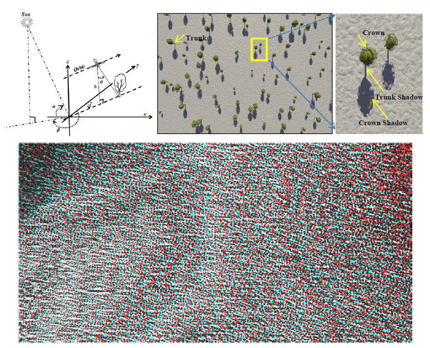
2.1. Features of the Mountainous Forest Landscapes

The relative terrain model is automatically generated by default in POV-Ray, based on the input of an 8-bit or 16-bit gray graphic image in a general format of gif, jpeg, png, tiff, and so on. However, the images simulated based on the default relative terrain model could only be used for visualization purpose. They could not be used for stereoscopic analysis like real remote sensing images due to the lack of geographical information. It is necessary to first define a geographical coordinate system and then build a georeferenced terrain model for the LandStereo model. The default coordinate system in POV-Ray is left-handed. The right-handed coordinates system could be built by rotating −90° along the x-axis and inversing the y-axis. The coordinates and height ranges are initially set from 0.0 through to 1.0. The georeferenced terrain model is defined in the LandStereo model, by the transformation of the relative terrain model, as
x = x 0 , n w + x i n c Δ x
y = y 0 , n w y i n r Δ y
z = h m i n + z i ( h m a x h m i n )
where ( x i , y i , z i ) and ( x , y , z ) are the coordinates of one point in the relative and georeferenced models, respectively. n c and n r are the number of samples and lines of input gray graphic image files, respectively. The Δ x and Δ y are the pixel sizes along x and y directions, respectively. ( x 0 , n w ,   y 0 , n w ) is the georeferenced coordinate of the northwest (upper left) corner of the input gray graphic image file;   h m a x and h m i n are the maximum and minimum elevations, respectively.
In the LandStereo model, each tree is defined by its coordinate, diameter at breast height, tree height, crown width, and crown length. The crown shape of each tree could be described vividly using the SDL (https://f-lohmueller.de/pov_tut/plants/plants_410e.htm). In order to minimize the computation load, the crown shape model proposed by Christoph Hormann (the coded is provided in the file of ..\scenes\advanced\landscape.pov) is adopted in the LandStereo [35]. A tree crown is described by a randomly carved ellipsoid, specified by crown width and crown length. In order to create unique optical textures for each tree, the other two smaller randomly carved concentric ellipsoids with random sizes are put inside the tree crown. The three concentric randomly carved ellipsoids are randomly rotated along their common vertical axis to generate different gap patterns within the tree crown and different shadow patterns. Figure 1 shows an example of a simulated image by describing the tree crowns using three embedded carved concentric ellipsoids. It is clear that the different crowns could exhibit different optical textures and shadows.
Spectral features of the mountainous forest landscapes also need to be defined for the simulation of vivid images. The software of POV-Ray provides user many options/tools to define the desired complex visual effects. Appendix A gives a brief description about how spectral features of the forest landscapes are defined in the LandStereo model, using the tools of POV-Ray. Please refer to the help documents of the software for more details.

2.2. Settings of the Observation Geometry

The georeferenced mountainous forest landscape can be defined in the LandStereo model by a terrain image and a tree list, as described in the last section. The next important section is to set the parameters of the observation system. POV-Ray provides examples of codes to simulate photos by setting the desired photo size (i.e., a number of lines and samples), positions, and orientations of a frame camera. However, images simulated by these code examples are for the purpose of visualization, but are insufficient for stereoscopic analysis like real remote sensing images. First, the typical optical sensor onboard the satellite is a linear pushbroom camera other than the frame camera. Second, the spatial resolution of simulated images could not be accurately calculated if the camera is defined as in the POV-Ray codes examples, because the critical physical variables are ignored, such as the focal length. In the LandStereo model, the observation system is defined by two parts, i.e., the camera parameters and the observation geometry. Typically, the spaceborne stereoscopic mission works on a pushbroom mode using linear charge-coupled-devices (CCD) composed of small detector elements [36]. The field of view of a linear camera could be defined by three parameters, including focal length f, dimension of a detector element Δ c , and a number of detector elements n c [36].
The observation geometry is defined by the positions of the light source and the view-point, as shown in Figure 2. The x-axis and the y-axis point to east and north, respectively. The sun as a light source is defined by the elevation angle φ and the azimuth angle β. β is defined relative to the north direction and increases along the clockwise direction. Therefore, the azimuth angle for the sun in the east, south, and west direction, should be 90°, 180° and 270°, respectively. The view-point is defined by the orbit height h, orbit heading angle γ, off-nadir view angle θ, along the orbit, as shown in Figure 2. The positive value of θ means looking forward along the flying direction. The starting point of the observation is set by co-ordinates of the central point of the first image line, i.e., ( x c , 0 , y c , 0 , z c , 0 ) . The co-ordinates of the view-point for each image line ( x c , j , y c , j ) could be calculated by the observation geometry as
x c , j = x c , 0 ( h z c , 0 ) tan θ sin γ + ( j 1 ) Δ sin γ
y c , j = y c , 0 ( h z c , 0 ) tan θ cos γ + ( j 1 ) Δ cos γ
Δ =   Δ c h / ( f cos 2 θ )
where Δ is the pixel size at ground level (or the ground sampling distance) and j is the line sequential number.

3. Building the Geometric Sensor Model

3.1. Description of the Geometric Sensor Model

Once the mountainous forest scene is set up and the observation geometry is defined by user provided parameters, multi-view optical images could be simulated by the LandStereo model using the ray-tracing technique. The next essential step for the stereo matching of the simulated multi-view optical images is to build the geometric sensor model. Building the geometric sensor model is one of the main tasks in photogrammetry. Most optical models for the simulation of spectral features of forest canopies do not include this step, since these models are not intended to simulate stereoscopic images. Geometric sensor model is used to describe the functional relationship between the two-dimensional image space (line, sample) and the three-dimensional georeferenced object space (latitude, longitude, elevation) [37]. The rational function model (RFM) is a kind of geometric sensor model, which uses ratios of polynomials to establish the relationship between the image space and the georeferenced object space. Appendix B gives the detailed form of RFM.
The RFM model is sensor-independent. Only the rational polynomial coefficients (RPC) of the RFM need to be updated for the images acquired by different satellites. Therefore, the RFM is broadly used in the state-of-art digital photogrammetric software packages. Typically, the RPC is composed of these 90 coefficients, including the 10 parameters used in the coordinate normalization and the 80 polynomial coefficients. For the stereo images simulated by the LandStereo model, the 10 parameters for coordinate normalization could be easily determined by the simulated image size, spatial coverage, and the elevation ranges of the imaging area, while the 80 polynomial coefficients needed to be determined. The iterative least-squares solutions, as proposed by Tao and Hu in [37], is used in the LandStereo model to solve for the 80 polynomial coefficients using the ground control points (GCP), whose image coordinates and object (georeferenced) coordinates are known.

3.2. Generation of the Ground Control Points

In order to calculate the RPC of the geometric sensor model for a simulated imagery, the GCP needs to be generated or calculated by a physical imaging process. The image coordinates of one ground point could be accurately calculated using the parameters of observation geometry and its georeferenced coordinates, i.e. to derive ( r i , c i ) from ( x i , y i , z i ) with known variables, including the starting point for the central point of first image line ( x c , 0 , y c , 0 , z c , 0 ) , view angle along orbit θ, orbit heading angle γ, focal length f, ground sampling distance Δ , and so on. In the theory of photogrammetry, the GCP could be calculated exactly by a collinearity equation using the observation geometry defined in the last section. For the convenience of understanding, the geometrical relationship between the ground object and its corresponding image pixel is provided in Appendix C. It is suggested that the GCP are evenly scattered within the spatial coverage of the simulated image and its elevation ranges [37].
Once the multi-view optical images are simulated and the corresponding geometric sensor model expressed by RPC is built, the stereo matching could be carried out using general commercial software, such as PCI, ERDAS, ENVI, and so on. The common points, i.e., projections of one ground point on the images of different views, are first identified on the basis of texture matching among multi-view optical images. The parallax is then measured by the identified common points. The elevation of a ground point could be calculated using the measured parallax and the geometric sensor model, i.e., RFM.

4. Validation Settings of the LandStereo Model

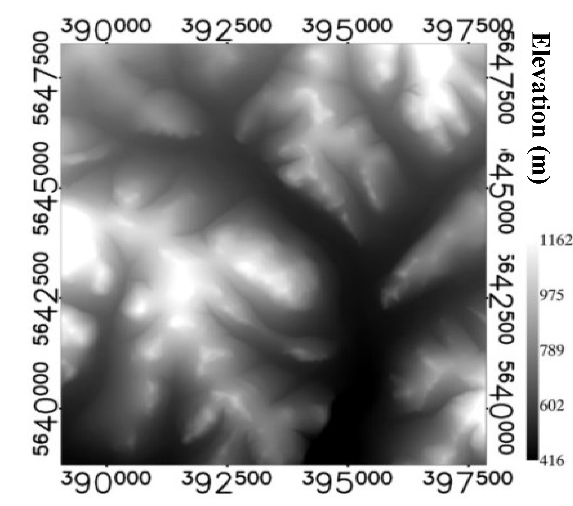
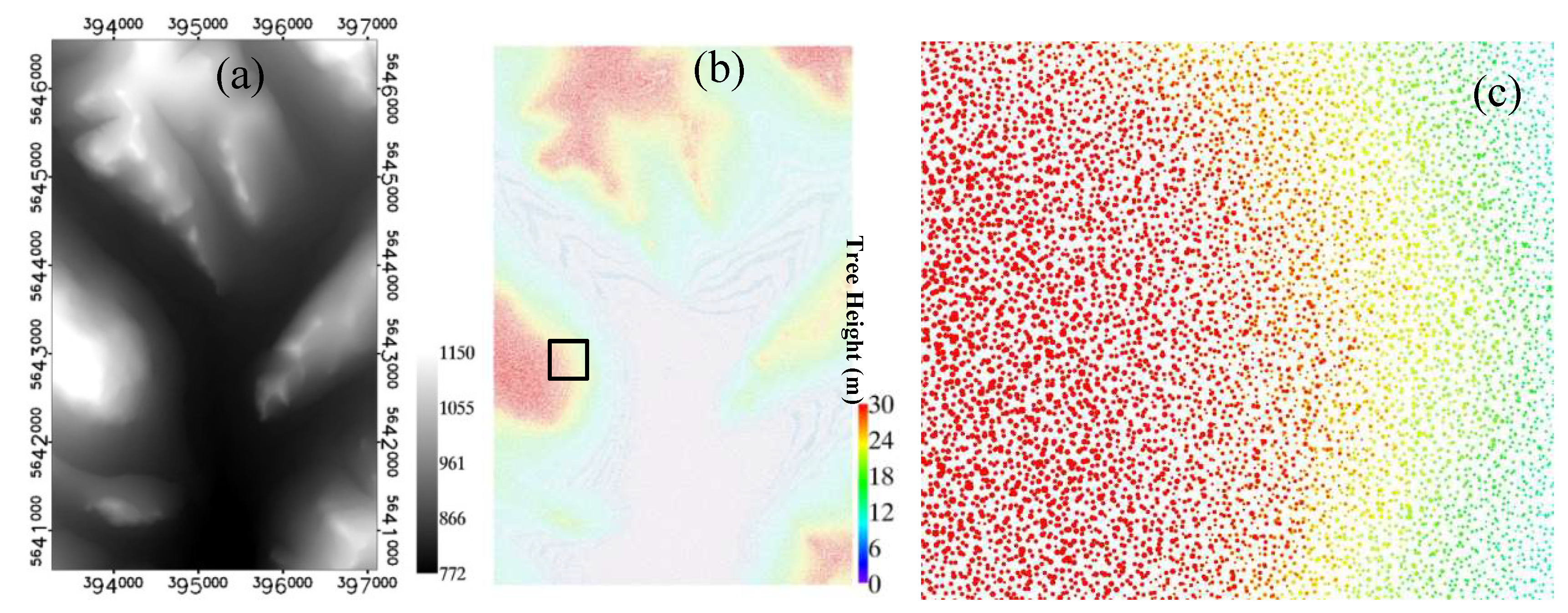
4.1. Simulated Landscapes

The LandStereo model has the capability to simulate the stereoscopic features of forest canopies over mountainous areas at landscape scales. In this paper, the model was verified by three scenes, including (a) forest landscapes on flat terrains (case 1); (b) bare mountains without any vegetation (case 2); and (c) mountainous forest landscapes (case 3). Appendix D shows the detailed workflow of the model validation. The first scene could examine the model’s performance in simulating the stereoscopic features of forest canopies without terrain influences. The second scene could validate the capability of the model to simulate the stereoscopic features of the terrains. The third scene was the most complicated one and the one that was nearest to the real forest scene, among all three scenes.
The third forest scene was built using a digital terrain model (DTM) and a tree list. The DTM used in this study was extracted from airborne LiDAR point cloud data. The point cloud was classified as the ground and non-ground points. The DTM with a resolution of 1 m was produced by the rasterization of the ground points. The size of the DTM was 9.559 km by 8.813 km. The maximum and minimum elevation was 1,162 m and 416 m, respectively, as shown in Figure 3.
The tree list provided the coordinates, the diameter at breast height (DBH), the tree height, crown width, and the crown length of each tree. It is difficult to measure each tree over such a large area. As pointed out in [38], the tree parameters could be generated using the forest growth models, such as the SIBBORK model, which is a type of spatially-explicit gap model [39]. The coordinates, species and DBH of each tree are the direct output of the forest growth model [39,40]. Regression relationships developed from the field data are used to estimate the tree height, crown depth, and width from the DBH [41]. In total, 842,121 trees were generated with a maximum tree height of 30.0 m and a minimum tree height of 5.0 m. The first scene was built by keeping the tree list but setting the elevations to be a constant, at 772.0 m. The second scene was built by keeping the DTM but removing all trees.

4.2. Simulation Parameters

Table 1 lists the parameters used in model simulation. The first four lines are the metadata of DTM, including data dimensions ( n c , n r ), spatial resolutions ( Δ x , Δ y ), elevation dynamic ranges ( h m a x ,   h m i n ), and the absolute geo-referenced (UTM 51N) coordinates of the upper left corner ( x 0 , n w , y 0 , n w ). The fifth line defined the direction of the light source (φ, β). The sixth and seventh lines described the camera parameters, including the focal length (f), size of the sensing elements (   Δ c ), the number of sensing elements of the linear CCD ( m c ), and the number of lines ( m r ) to be simulated. The eighth to tenth lines depict the observation geometry, including the coordinates of the starting observation point ( x c , 0 ,   y c , 0 ), flying height (h), flying direction (γ), view angle (θ), and image resolution ( Δ ). The elevation of the starting point ( z c , 0 ) could be read from the DTM by the positions of the starting point. The size of the sensing elements in Table 1 is for the nadir view. For the non-nadir view, it was adjusted by Equation (6), according to the view angle to achieve the specified image resolution.
The geometric sensor model was developed using the terrain-independent method [37]. The GCP were evenly distributed across the full extent of the simulated image, in a grid of 20 columns by 30 rows. Six elevation layers were used ranging from 500 m to 1200 m. The image coordinates and georeferenced coordinates of the GCP were calculated through the physical imaging process as described in Section 3.2. The RPC was solved through the fitting of RPM using GCP through the iterative least square estimations. The checking points were generated in a similar way, but with more density in each dimension. The checking points were generated using 37 columns by 59 rows, with 11 elevation layers. Therefore, in total 3600 GCP were generated for the calculation of RPC and 24013 checking points were generated for each simulated image to evaluate the accuracy of the geometric sensor model expressed by the RPC.

5. Validation Results of the LandStereo Model

The spatial coverage of the simulated image was 3.84 km in width and 6.0 km in length, according to the setting of the simulation parameters in Table 1. The DTM within the simulated area is shown in Figure 4a. The canopy height model (CHM) produced, based on the tree list, is shown in Figure 4b. Figure 4c is a subset of Figure 4b, over the area marked by the black square. The background is white and each color dot indicates one tree.

5.1. Accuracy of the Sensor Model

Figure 5 shows the accuracy of the geometric sensor model described by the derived RPC. Figure 5a–c are the maximum error of the geometric sensor model, for images simulated with view angles of 0°, 20°, and −20°, respectively, i.e., the maximum difference between the image coordinates of the check points calculated by the physical imaging process and those predicted by the RPC. The horizontal axis is the number of iterations for the estimation of RPC, using iterative least-square-estimations. One set of the RPC was produced in each iteration and it was used as the initial value of the next iteration. It can be seen that the accuracy of the RPC converged after 5–6 iterations. Figure 5d–g are the root mean square error (RMSE) of the geometric sensor model, for the images simulated with a view angle of 0°, 20°, and −20°, respectively. It can be seen that the maximum error of the GCP and the checking points converged at around the 0.07 pixel in the Y direction and around 0.04 pixel in the X directions, for all of the three view angles. The RMSE converged at around the 0.03 pixel in the Y direction and around the 0.02 pixel in the X direction for all three view angles. The accuracy was comparable with that reported in [37].

5.2. Accuracy of the Flat Forest Landscapes

Figure 6 shows the simulated image of the first scene (i.e., the flat forest landscape). Figure 6a is the entire simulated nadir image with the true color. Figure 6b is a subset of the nadir image marked by the black rectangle in Figure 6a. The tree crowns, shadows, and ground surface are clearly visible in Figure 6b. Figure 6c–e show an enlarged gray image (i.e., the summation of red, green, and blue channels) simulated with different view angles of 0° (nadir), 20° (forward), and −20° (backward), respectively. The red crosses in Figure 6c–e indicate the same ground position. It can be seen that tree shadows (darker pixels) remained at the same position in all of three view angles but the positions of the tree crowns (pixels with medium gray values) relative to its shadow, changed with the view angle, along the vertical direction. Figure 6f is a composite image of Figure 6c–e in red, green, and blue channels, respectively. The displacement caused by the different view angles is more obvious in Figure 6f. The displacement exhibited on Figure 6c to Figure 6f, clearly demonstrates that the LandStereo model is capable of simulating the stereoscopic features (i.e., parallax) of forest canopies.
The simulated images were stereo matched using the extraction module of the digital elevation model provided in the commercial software ENVI. Figure 7 shows the spatial distribution of the point cloud (common points), extracted using the different view combinations. Figure 7a is the subset of the nadir image. Figure 7b is the point cloud identified from the stereo image pair of the nadir and the forward (NF), over the same area as Figure 7a. The white pixel indicates that the pixel matching was successful between the image pair, while the black pixels indicate a failure in pixel matching. Figure 7c,d was similar with Figure 7b but was extracted from an angle combination of NB (nadir and backward) and FB (forward and backward), respectively. Figure 7e is the composite image of Figure 7b–d in red, green, and blue channels, respectively. It can be seen that more points were identified in the image pair of NF and NB, than that in FB. This could be attributed to the changes of the image textures between the different combinations of observation angles. The stereo matching was easier on the images with a less change of image textures. It was not difficult to understand that the changes of the image textures were more severe for the images with larger differences of observation angles. The angle difference between NF and NB was only 20°, while that between FB was 40°. Therefore, it could be anticipated that lesser point could be identified in FB, through automatic image matching than what could be identified in NF and NB.
Figure 7e shows the complementary effect between the different view angle combinations. The white pixel indicated that the common pixel was successfully identified in all of the three combinations, while the black pixels indicate that no common pixel could be identified in any of the view combinations. The colorful pixel meant a common pixel was identified in one or two view combinations. Comparing Figure 7e with Figure 7a, it was easily observed that the white pixels were mostly located within the forest gaps, while the colorful pixels were located on the tree crowns. Therefore, it could be concluded that the synergy of the point cloud extracted from different view combinations was helpful for increasing the point cloud density and in further improving the description of the forest spatial structures.
Figure 8 shows the vertical distribution of the point cloud from different view combinations, for different forest stands with a size of 30 m by 30 m. The vertical axis was the elevation while the horizontal axis was the normalized point number. The horizontal bars with different colors indicated portions of the points from different view combinations. Theoretically, there should have been 900 points for each view combination and in total there should have been 2700 points in each forest stand. The vertical width of each colorful horizontal bar was 1.0 m. All bars were normalized by the one with the maximum point numbers. The elevation of the ground surface was 772.0 m. The blue line was the vertical distribution of the forest canopy tops calculated from the tree list. Figure 8a shows the vertical distribution of the point cloud extracted over a taller forest stand. It could be seen that the point cloud was mainly located near the canopy top. This was reasonable because taller trees have larger crowns and higher canopy coverage as described in the building of forest scenes. Figure 8b shows the vertical distribution of the point cloud extracted over a forest stand with medium heights. The point cloud could capture the ground surface through forest gaps. Therefore, the point cloud distributed between the ground surface and the canopy tops. Figure 8c shows the vertical distribution of the point cloud extracted over a shorter forest stand. More points were located on the ground surface than the forest canopy top.
Figure 9 shows the forest height extracted from the synergy of multi-view stereo images simulated from the first scene (i.e., flat forest landscape). Figure 9a is an image of the number of common points within a resolution cell of 30 m. As depicted previously, there should be 2700 points in total in each 30 m pixel, since the point cloud had a pixel size of 1 meter. Results showed that the maximum number of common points identified was 2137 and a shorter forest had more common points than a taller forest. Figure 9b shows the image of the height of 90% of points (H90), i.e., the number of common points below this height was 90% of the total number of points within a pixel. It could be observed from Figure 8 that the upper boundary of a vertical histogram of the common points was located near the forest canopy top, while some false common points occasionally appeared due to the incorrect match between the stereo image pairs, as shown at the elevation of 799.0 m in Figure 8a. Therefore, H90 was selected as an index for describing the forest height. Figure 9c shows the image of H90 produced from the tree list. The canopy height model with a resolution of 1.0 m was first generated according to the tree list. Then, the vertical histogram of the CHM pixels within each 30 m by 30 m forest stand was calculated. The height of H90 was determined in the same way as that of Figure 9b. Figure 9d shows the scattering plot of Figure 9b against Figure 9c. They were highly correlated with each other; R2 = 0.96 and RMSE = 0.99 m.

5.3. Accuracy of the Bare Mountainous Landscapes

Figure 10 shows the stereoscopic features of the bare terrains, simulated using the LandStereo model and parameters of the second scene in Table 1 (i.e., bare mountains without any vegetation). The geometric sensor model was the same as that of the first scene, because the simulation parameters were not changed. Figure 10a shows the simulated gray nadir image. Figure 10b shows the stereoscopic image composed by taking epipolar images of the forward view (in red) and that of backward view (in green and blue). Stereo vision can be seen when Figure 10b is observed by red–blue 3D glasses. The colorful pixels were caused by the parallax. Figure 10c is the scatter plot of the elevations extracted from the simulated stereo imagery and the input DTM as shown in Figure 4a. It could be seen that all pixels scattered along the 1:1 diagonal line. They were highly correlated with R2 = 0.9997 and RMSE = 1.32 m. Figure 10d shows the histogram of the elevation difference between the estimation and the true value. There is no doubt that the LandStereo model showed a good performance in the simulation of stereoscopic features of the terrains.

5.4. Accuracy of the Mountainous Forest Landscapes

Figure 11 shows the stereoscopic features of mountainous forest landscapes (the third scene) simulated using the LandStereo model and the parameters in Table 1. The geometric sensor model was the same as that of the first scene, because the simulation parameters had no change. Figure 11a shows the simulated nadir image with the true color. Compared Figure 6a with Figure 11a, it can be seen that the terrain features are clearly exhibited in the latter. Figure 11b shows the stereoscopic image composed in the same way as Figure 10b. The subset of Figure 11b over the area covered by the white rectangle is shown as Appendix E. More color pixel could be observed, due to the complicated parallax of forest canopies. Figure 11c shows the image of the number of common points in each forest stand (i.e., 30 m pixel). It could be seen that more common points were identified over the flat area or gentle terrains, but fewer common points could be identified over the steep mountains. This should be attributed to the severe changes of image textures and larger parallax, over the steep mountains than the flat terrains. Figure 11d shows the scattering plots of the heights of the forest canopy tops extracted from the multi-view stereo imagery against the heights of forest canopy top calculated from the tree list. The extracted forest height and its measurements were highly correlated with R2 = 0.92 and RMSE = 1.15 m.
Figure 6, Figure 7, Figure 8, Figure 9, Figure 10, Figure 11 show the results from the simulated stereo images of the three scenes, i.e., the flat forest landscape, bare mountains without any vegetation, and the mountainous forest landscapes. These results clearly showed a good performance of the LandStereo model in the simulation of stereoscopic features of forest canopies, over mountainous areas, at landscape scales.

6. Discussions

Generally, for remote sensing models simulating multispectral features of vegetation, the comparison of the simulated results to the real data is an essential way to make model validations. The input in such types of models are the forest scenes and the spectral information of vegetation components, such as leaves, branches, and so on, while the output of the model is the spectral data of a forest stand. We do not know what the simulated multispectral features of the forest stand should be, if no real remote sensing data is used. Therefore, a comparison of the simulated data to real data is necessary for the validation of such models. The LandStereo model proposed in this study was used to simulate the stereoscopic features rather than the multispectral features. The stereoscopic features of remote sensing images were directly determined by the ground surface elevation, the tree size, and the observation geometry. For the given observation geometry (i.e., the geometrical sensor model expressed by RPC), the ground surface elevation and tree sizes should be correctly extracted from the simulated stereoscopic features, if the proposed model is valid. It is impossible to extract the ground surface elevation and tree size if the proposed model is invalid. The ground surface elevation (i.e., digital surface model) and tree sizes are the input of the proposed model. The input ground surface elevation and parameters of the trees above the surface, is the “real data”. Therefore, a comparison of the ground surface elevation and canopy height extracted from the simulated stereoscopic features to the model input is enough for the validation of the proposed model.
The development of the LandStereo model and the analysis of the model simulations were interdisciplinary. The simulation of the stereoscopic images belongs to the subject of computer graphics; the development of a geometric sensor model is a task of photogrammetry; the extraction of the parallax by image matching is the work of computer vision. The LandStereo combines the knowledge of these subjects to simulate stereoscopic images for the monitoring of forest spatial structures. The LandStereo model is not just a simple collection of the existing tools in different subjects, rather it is a creative unification of the interdisciplinary knowledge. It is impossible to simulate images applicable to stereo matching without these creative works. The LandStereo model could work as a virtual satellite to capture the stereo imagery of the predefined landscapes with the given system parameters as shown in Table 1. This model could provide an important set of image simulations that help examine the impact of the viewing geometry, on the measurement of the forest structure from spaceborne stereogrammetry.
In this study, the crown shapes were modeled using three embedded carved concentric ellipsoids. This was not the only choice. The POV-Ray has great power to simulate complicated and vivid forest scenes (http://hof.povray.org/). There are many studies that have been working on the simulation of real trees using POV-Ray. Many tree models have been developed (such as http://povrayscrapbook. awardspace.com/index.html). These trees could easily be incorporated into the simulation of the LandStereo model.
The stereo imagery simulated in this study was optical imagery. The effect of the atmosphere on image quality was unavoidable. The POV-Ray was effective at simulating atmospheric conditions, such as fog, dust, haze, or visible gas (http://www.povray.org/documentation/ view/3.7.0/252/#l129). Therefore, the LandStereo model should be potentially used to analyze the effects of atmospheric conditions on the measurements of the forest spatial structure, using stereo imagery.
The multi-view observation could produce both the stereoscopic information and the multi-angle spectral information (i.e., the Bidirectional Reflectance Distribution Function). The LandStereo model simulated image using the ray-tracing embedded in the POV-RAY, and had the potential to simulate the BRDF of a visible spectrum of a forest scene. This paper focused on the simulation of stereoscopic features as indicated by the paper title. Its performance on the simulation of BRDF will be explored in future research work.
There were two modes for the acquisition of stereo imagery by spaceborne stereoscopic systems. The first was the along-track stereoscopic observations, i.e., the parallax information was extracted using images acquired by different cameras onboard the same satellite but pointing to different angles along track. The AOLS/PRISM, Chinese ZY-3, and the ASTER all worked in this mode. The second was the stereoscopic observations by the across-track satellite stereo pair. The spaceborne stereoscopic systems having super high spatial resolutions such as worldview imagers work on this mode, because it was difficult to mount two cameras with large telescopes on the same satellite. It could be seen from Equations (4)–(6) that only the along-track angle θ was considered in determining the view direction. Therefore, the current version of the LandStereo model could only be used to simulate the along track stereoscopic observations. The LandStereo model would need to be modified for the simulation of stereoscopic observations, from the arbitrary viewing directions.
Two types of cameras were typically used in the acquisition of remote sensing images, i.e., pushbroom and frame cameras. The pushbroom cameras are widely used on satellites, while the frame cameras are widely used on the airborne platforms, such as the manned or the unmanned aerial vehicle (UAV). The POV-Ray had the capability to simulate optical images acquired by both types of cameras. However, the LandStereo model proposed in this study only accurately defined the observation geometry of the along-track pushbroom cameras. Therefore, the LandStereo model of the current version could not be used to simulate the frame cameras. For the theoretical analysis of stereo imagery acquired by frame cameras, the LandStereo model would be enhanced by modeling the observation geometry of frame cameras in future works.
There were two scenarios for the calculation of RPCs, i.e., terrain-independent and terrain-dependent. Tao, C.V., and Hu Y. (2001) reported that 80 GCPs were enough for the terrain-dependent scenarios because accuracy would not be improved as such if more number of GCPs were used. There was no need to spend more effort to collect more GCPs considering the cost [37]. In this study, the physical sensor parameters were known as shown in Table 1, therefore, the terrain-independent scenario was applied. For this case, the GCPs should be determined by the image grid and the elevation layers, so that the GCPs points are evenly distributed across the full extent of the image. The number of GCPs could be freely determined, as long as it is more than the minimum requirement.
The performance of the stereo matching algorithm is an important factor affecting the quality of the point cloud extracted from the stereo imagery. Many different algorithms of stereo matching have been developed in the computer version as well as in photogrammetry [42,43]. This study only used the one adopted by the commercial software ENVI in the extraction module of the digital elevation model. The accuracy of canopy height extracted by the point cloud might be improved if more proper algorithm of stereo matching is used. It was worthwhile to evaluate the performances of the different algorithms of stereo matching on the extraction of the forest canopy heights.
The parameters used in the model validation, as shown in Table 1, were not set for any specific satellite, rather were used for the approximation of several on-orbit satellites. For example, the orbit height of 500 km, approximates that used in the Chinese ZY-3, i.e., 505.984 km [44]. The combination of focal length, element size, and orbit height, produced a spatial resolution of 1.0 m, which approximated that of the IKONOS Satellite Sensor, [45]; the view angle was the same as that of SPOT5, i.e., ±20° [46].
One interesting phenomena observed in Figure 8b,c was that the point cloud extracted from the view combination of forward and backward was mostly located on the ground surface, except for the forest canopy tops. Theoretically, the common part which could be seen from both the forward and backward views, should have been the forest canopy tops, if the top was relatively flat, so that the canopy tops were the matching points. However, the results showed that it was difficult to identify the common points on the forest canopy tops by an automatic image matching algorithm due to the severe changes of the image textures of the forest canopy top between the forward and the backward views. Therefore, a more common point was unexpectedly identified on the ground surface than at the forest canopy top.

7. Conclusions

The number of spaceborne stereoscopic systems has been growing in recent years. However, these systems work on different viewing angles and image spatial resolutions. A theoretical model is needed for the systematical analysis of their performance on the depiction of forest canopy structures, especially over the complicated mountainous landscapes. Considering the fact that those mostly found in the optical models of remote sensing, focus on the simulation of multispectral features, this study proposed a new model, referred to as the LandStereo model, using the ray tracing technique, to simulate the stereoscopic features of mountainous forest landscapes. The model was validated by making the simulations over flat forest landscapes, bare terrain landscapes, and mountainous forest landscapes. For the flat forest landscape, the height of the forest canopy top were extracted from the simulated stereo imagery, with R2 = 0.96 and RMSE = 0.99 m; the elevation of the ground surface were extracted from the simulated stereo imagery of bare ground, with R2 = 0.9997 and RMSE = 1.32 m. Given the elevation of the ground surface, the height of the forest canopy top were extracted from the simulated stereo imagery of the mountainous forest landscapes, with R2 = 0.92 and RMSE = 1.15 m. It could be seen that the simulated stereo imagery could be used for the extraction of the ground surface elevations and the height of the forest canopy top. These simulated results clearly demonstrated that the LandStereo model worked well in simulating stereoscopic features of both terrains and forest canopies, at landscape scales.
The LandStereo model could work as a virtual satellite to capture stereo imagery of predefined landscapes with the given system parameters. The LandStereo model is capable of creating more simulations to understand the influences of view angles, image resolutions, terrain conditions, and temporal changes on the extraction of forest heights, using spaceborne stereo imagery over different forest types. Such relevant studies will be carried out in our future research endeavors.

Author Contributions

Conceptualization, W.N.; methodology, W.N.; software, Z.Z.; validation, W.N., Z.Z., and G.S.; formal analysis, W.N. and Z.Z.; investigation, W.N.; writing—original draft preparation, W.N.; writing—review and editing, G.S.; visualization, Z.Z.; supervision, Q.L.; funding acquisition, Q.L.

Funding

This research was funded in part by the National Key R&D Program of China (Grant No. 2017YFA0603002), National Basic Research Program of China (Grant No. 2013CB733401), and in part by the National Natural Science Foundation of China (Grant Nos. 41471311, 41371357, 41301395).

Acknowledgments

Special thanks to Paul M Montesano from NASA/NSFC for his help on valuable suggestions in the paper preparation.

Conflicts of Interest

The authors declare no conflict of interest.

Appendix A. Spectral Features of Mountainous Forest Landscapes

The spectral feature of an object is defined by the statement of “texture” in the POV-Ray. The “texture” is composed by three keywords, including “pigment”, “normal”, and “finish”. The “pigment” defines the color of an object by setting the values of the red, green, and blue channels. The “normal” is used to select a method of simulating various patterns of bumps, dents, ripples, or waves, by modifying the surface normal vector. The calculation of reflection depends on the surface normal vectors. The POV-Ray provides many predefined patterns of normal vectors, for the users to select. The “finish” describes the reflective properties of objects, which are further defined by “specular”, “ambient”, or “diffuse”. The “specular” defines a credible spreading of the highlights occurring near the object horizons. The value of “specular” ranges between 0.0 and 1.0, where 1.0 causes complete saturation to the light source’s color at the center of the highlight, and 0.0 gives no highlight. The “ambient” is used to define the light in the shadowed areas, from a diffuse reflection of other objects. The “diffuse” is used to control how much of the light is reflected via diffuse reflection, directly, from any light sources.
The LandStereo model adopted the values proposed in the work of Christoph Hormann. For trees, the “pigment” is—(0.4, 0.2, and 0.05). The “normal” uses the predefined pattern representing a very smooth surface, like random noise. The “specular” is 0.3 and the “diffuse” is 0.5. For the ground surface, the “pigment” is—(1.1, 0.7, and 0.3); the “normal” uses the predefined pattern of “granite” which creates a bumpy surface that looks like rough stone. The “specular” is 0.06 and the ambient is—0.08, 0.09, and 0.14.

Appendix B. The Rational Function Model

In the RFM model, for the ground object point i, both its coordinates in image space ( r i , c i ) and in object space ( x i , y i , z i ) are firstly normalized to the range of −1.0 to +1.0, as
R i = r i r 0 r s   ,   C i = c i c 0 c s ,   X i = x i x 0 x s ,   Y i = y i y 0 y s ,   Z i = z i z 0 z s
where r 0 ,   c 0 and r s ,   c s are the offsets and scale values for the normalization of image coordinate, respectively, while x 0 , y 0 , z 0 and x s , y s , z s are the offsets and scale values for the normalization of object coordinates, respectively. For the images simulated by LandStereo,
r 0 = r s = 0.5 m r ,   c 0 = c s = 0.5 m c
x 0 = 0.5 ( x m a x + x m i n ) ,   y 0 = 0.5 ( y m a x + y m i n ) ,   z 0 = 0.5 ( h m a x + h m i n )
x s = 0.5 ( x m a x x m i n ) ,   y s = 0.5 ( y m a x y m i n ) ,   z s = 0.5 ( h m a x h m i n )
where m r and m c is the number of lines and samples of simulated image, respectively; x m a x ,   x m i n ,   y m a x , and y m i n are dynamic ranges of coordinates of the spatial coverage of the simulated image; h m a x and h m i n are the same as that in Equation (3), i.e., the maximum and minimum elevations within the spatial coverage of the simulated image, respectively.
The mathematical relationship between the normalized image coordinates ( R i , C i ) and object coordinates ( X i , Y i , Z i ) in the RFM model can be expressed as
R i = p 1 ( X i , Y i , Z i ) p 2 ( X i , Y i , Z i ) ,   C i = p 3 ( X i , Y i , Z i ) p 4 ( X i , Y i , Z i )
p l = a 1 , l + a 2 , l X i + a 3 , l Y i + a 4 , l Z i + a 5 , l X i Y i + a 6 , l X i Z i + a 7 , l Y i Z i + a 8 , l X i 2 + a 9 , l Y i 2 + a 10 , l Z i 2 +   a 11 , l X i Y i Z i + a 12 , l X i 3 + a 13 , l X i Y i 2 + a 14 , l X i Z i 2 + a 15 , l X i 2 Y i + a 16 , l Y i 3 + a 17 , l Y i Z i 2 + a 18 , l X i 2 Z i + a 19 , l Y i 2 Z i + a 20 , l Z i 3
where l = 1, 2, 3, 4. p l defines the transformation from ( X i , Y i , Z i ) to ( R i , C i ) by the 20-term cubic form polynomial shown above.

Appendix C. Geometry for the Generation of GCP

The GCPs are required for building a camera model (RPC), by providing exact relations between image coordinates of the ground points and the corresponding georeferenced coordinates. These relations can be exactly simulated. The central content is how to derive ( r i , c i ) from ( x i , y i , z i ) , with the known variables, including the starting point observed by the central point of the first image line ( x c , 0 , y c , 0 , z c , 0 ) , view angle along orbit θ, orbit heading angle γ, focal length f , ground sampling distance Δ , and so on. For the convenience of understanding for readers who are not quite familiar with the theory of photogrammetry, the geometrical relationship between ground object location and its corresponding image pixel is shown in Figure A1. As shown in Figure A1a, point A is the starting point (i.e., the center of the first line of the simulated image), point B is the observed target point, point C is the projection of point B in the horizontal plane, point D and point F are the projections of point C and point B, in the plane defined by the z-axis and the flying orbit, respectively. Point M, point G, and point P are the view-point through point A, point D, and point F, respectively; point E is the intersection point of line PF and line AD. It can be seen that the line coordinate of one ground point on the simulated image ( r i ) could be calculated as
r i = AE / Δ ,   A E = AD + DE ,   DE = ( z i z c , 0 ) tan θ
A D = AC c o s φ ,   A C = ( x i x c , 0 ) 2 + ( y i y c , 0 ) 2
c o s φ = cos ( 90 ° μ γ ) = sin ( μ + γ ) = sin μ cos γ + cos μ sin γ
sin μ = ( y i y c , 0 ) / A C ,   cos μ = ( x i x c , 0 ) / A C
Writing the distance from the projection of ground point B in image space, to the central point of image line j, along the sample direction, as Δ s , it can be seen from Figure A2b that
c i = Δ s / Δ c + 0.5 m c
Δ s B F = f ( h z i ) / cos θ   Δ s = f ( h z i ) / cos θ   B F
B F = ± ( x i x F ) 2 + ( y i y F ) 2
x F = x c , j + N F sin γ , y F = y c , j + N F cos γ
N F = ( h z i ) tan θ
The r i in Equation (A6) is the variable j in Equations (4) and (5). Therefore, the position of the view-point ( x c , j , y c , j , h ) for point ( x i , y i , z i ) can be calculated using Equations (4) and (5). Supposing that pixels in each image line are sequentially numbered from left to right with a center value of zero, the value of BF is negative when point B is on the left side of point F, looking along the flying direction. The transformation from ( x i , y i , z i ) to ( r i , c i ) could be done using equations (A6) through (A15).
Figure A1. Schematic diagram for the geometrical relationship between a ground object and its corresponding image pixel. (a) Observation geometry for z i z c , 0 , a point A ( x c , 0 , y c , 0 , z c , 0 ) on the horizontal plane, and a target point B ( x i , y i , z i ) above the plane; point C ( x i , y i , z c , 0 ) is the projection of point B on the horizontal plane, point D and point F are the projection of point C and point B in the plane defined by the z-axis and the flying orbit, respectively; point M, point G, and point P are the view-points through point A, point D, and point F, respectively; point E is the intersection point of line PF and line AD; and (b) the geometrics in imaging plane, point B, point F, and point P are defined the same as in (a), point N is the projection of point P in the horizontal plane.
Remotesensing 11 01222 g0a1

Appendix D. Detailed Workflow of the LandStereo Validation

Figure A2. Detailed workflow of the LandStereo validation.
Remotesensing 11 01222 g0a2

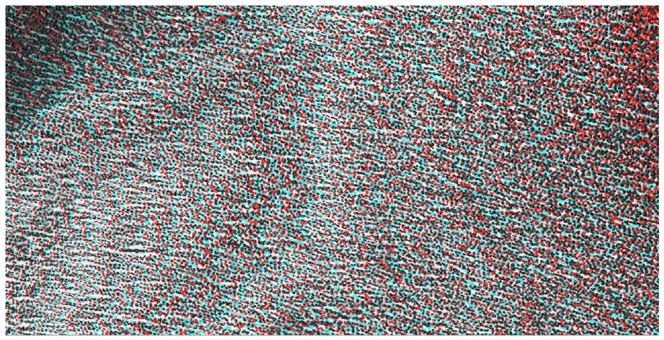
Appendix E. Subset of an Anaglyph Stereoscopic Image

Figure A3. Subset of an anaglyph stereoscopic image related to the individual tree level scale, covered by the white rectangle in Figure 11b.
Remotesensing 11 01222 g0a3

References

  1. Dunn, R.E.; Stromberg, C.A.E.; Madden, R.H.; Kohn, M.J.; Carlini, A.A. Linked canopy, climate, and faunal change in the cenozoic of patagonia. Science 2015, 347, 258–261. [Google Scholar] [CrossRef] [PubMed]
  2. Purves, D.; Pacala, S. Predictive models of forest dynamics. Science 2008, 320, 1452–1453. [Google Scholar] [CrossRef]
  3. Hall, F.G.; Bergen, K.; Blair, J.B.; Dubayah, R.; Houghton, R.; Hurtt, G.; Kellndorfer, J.; Lefsky, M.; Ranson, J.; Saatchi, S.; et al. Characterizing 3d vegetation structure from space: Mission requirements. Remote Sens. Environ. 2011, 115, 2753–2775. [Google Scholar] [CrossRef]
  4. Qi, W.L.; Dubayah, R.O. Combining tandem-x insar and simulated gedi lidar observations for forest structure mapping. Remote Sens. Environ. 2016, 187, 253–266. [Google Scholar] [CrossRef]
  5. Le Toan, T.; Quegan, S.; Davidson, M.W.J.; Balzter, H.; Paillou, P.; Papathanassiou, K.; Plummer, S.; Rocca, F.; Saatchi, S.; Shugart, H.; et al. The biomass mission: Mapping global forest biomass to better understand the terrestrial carbon cycle. Remote Sens. Environ. 2011, 115, 2850–2860. [Google Scholar] [CrossRef]
  6. Carreiras, J.M.B.; Shaun, Q.G.; Toan, T.L.; Minh, D.H.T.; Saatchi, S.S.; Carvalhais, N.; Reichstein, M.; Scipal, K. Coverage of high biomass forests by the esa biomass mission under defense restrictions. Remote Sens. Environ. 2017, 196, 154–162. [Google Scholar] [CrossRef]
  7. Slater, J.A.; Heady, B.; Kroenung, G.; Curtis, W.; Haase, J.; Hoegemann, D.; Shockley, C.; Tracy, K. Evaluation of the New Aster Global Digital Elevation Model; National Geospatial-Intelligence Agency: Virginia, VA, USA, 2009. [Google Scholar]
  8. Berthier, E.; Toutin, T. Spot5-hrs digital elevation models and the monitoring of glacier elevation changes in north-west canada and south-east alaska. Remote Sens. Environ. 2008, 112, 2443–2454. [Google Scholar] [CrossRef]
  9. Tadono, T.; Shimada, M.; Murakami, H.; Takaku, J. Calibration of prism and avnir-2 onboard alos “daichi”. IEEE Trans. Geosci. Remote Sens. 2009, 47, 4042–4050. [Google Scholar] [CrossRef]
  10. Ni, W.J.; Sun, G.Q.; Ranson, K.J. Characterization of aster gdem elevation data over vegetated area compared with lidar data. Int. J. Digit. Earth 2015, 8, 198–211. [Google Scholar] [CrossRef]
  11. St-Onge, B.; Hu, Y.; Vega, C. Mapping the height and above-ground biomass of a mixed forest using lidar and stereo ikonos images. Int. J. Remote Sens. 2008, 29, 1277–1294. [Google Scholar] [CrossRef]
  12. Neigh, C.S.R.; Masek, J.G.; Bourget, P.; Cook, B.; Huang, C.Q.; Rishmawi, K.; Zhao, F. Deciphering the precision of stereo ikonos canopy height models for us forests with g-liht airborne lidar. Remote Sens. 2014, 6, 1762–1782. [Google Scholar] [CrossRef]
  13. Montesano, P.M.; Neigh, C.; Sun, G.Q.; Duncanson, L.; Van Den Hoek, J.; Ranson, K.J. The use of sun elevation angle for stereogrammetric boreal forest height in open canopies. Remote Sens. Environ. 2017, 196, 76–88. [Google Scholar] [CrossRef] [Green Version]
  14. Ni, W.; Ranson, K.J.; Zhang, Z.; Sun, G. Features of point clouds synthesized from multi-view alos/prism data and comparisons with lidar data in forested areas. Remote Sens.Environ. 2014, 149, 47–57. [Google Scholar] [CrossRef]
  15. Dandois, J.; Olano, M.; Ellis, E. Optimal altitude, overlap, and weather conditions for computer vision uav estimates of forest structure. Remote Sens. 2015, 7, 13895–13920. [Google Scholar] [CrossRef]
  16. Fujisada, H.; Urai, M.; Iwasaki, A. Technical methodology for aster global dem. IEEE Trans. Geosci. Remote Sens. 2012, 50, 3725–3736. [Google Scholar] [CrossRef]
  17. Wallerman, J.; Fransson, J.E.S.; Bohlin, J.; Reese, H.; Olsson, H. Forest mapping using 3d data from spot-5 hrs and z/i dmc. In Proceedings of the IEEE International Geoscience and Remote Sensing Symposium, Honolulu, HI, USA, 25–30 July 2010; pp. 64–67. [Google Scholar]
  18. Kocaman, S.; Gruen, A. Orientation and self-calibration of alos prism imagery. Photogramm. Rec. 2008, 23, 323–340. [Google Scholar] [CrossRef]
  19. Imai, H.; Katayama, H.; Sagisaka, M.; Hatooka, Y.; Suzuki, S.; Osawa, Y.; Takahashi, M.; Tadono, T. A conceptual design of prism-2 for advanced land observing satellite-3(alos-3). SPIE Remote Sens. 2012. [Google Scholar] [CrossRef]
  20. Slater, J.A.; Heady, B.; Kroenung, G.; Curtis, W.; Haase, J.; Hoegemann, D.; Shockley, C.; Tracy, K. Global assessment of the new aster global digital elevation model. Photogramm. Eng. Remote Sens. 2011, 77, 335–349. [Google Scholar] [CrossRef]
  21. Li, X.W.; Strahler, A.H. Geometric-optical bidirectional reflectance modeling of a conifer forest canopy. IEEE Trans. Geosci. Remote Sens. 1986, 24, 906–919. [Google Scholar] [CrossRef]
  22. Chen, J.M.; Leblanc, S.G. A four-scale bidirectional reflectance model based on canopy architecture. IEEE Trans. Geosci. Remote Sens. 1997, 35, 1316–1337. [Google Scholar] [CrossRef]
  23. Qin, W.H.; Gerstl, S.A.W. 3-d scene modeling of semidesert vegetation cover and its radiation regime. Remote Sens. Environ. 2000, 74, 145–162. [Google Scholar] [CrossRef]
  24. Ni, W.G.; Li, X.W.; Woodcock, C.E.; Caetano, M.R.; Strahler, A.H. An analytical hybrid gort model for bidirectional reflectance over discontinuous plant canopies. IEEE Trans. Geosci. Remote Sens. 1999, 37, 987–999. [Google Scholar]
  25. Gastellu-Etchegorry, J.P.; Martin, E.; Gascon, F. Dart: A 3d model for simulating satellite images and studying surface radiation budget. Int. J. Remote Sens. 2004, 25, 73–96. [Google Scholar] [CrossRef]
  26. Huang, H.G.; Qin, W.H.; Liu, Q.H. Rapid: A radiosity applicable to porous individual objects for directional reflectance over complex vegetated scenes. Remote Sens. Environ. 2013, 132, 221–237. [Google Scholar] [CrossRef]
  27. Qi, J.B.; Xie, D.H.; Yin, T.G.; Yan, G.J.; Gastellu-Etchegorry, J.P.; Li, L.Y.; Zhang, W.M.; Mu, X.H.; Norford, L.K. Less: Large-scale remote sensing data and image simulation framework over heterogeneous 3d scenes. Remote Sens. Environ. 2019, 221, 695–706. [Google Scholar] [CrossRef]
  28. Farmer, D. Ray-tracing and pov-ray. Dr Dobbs J. 1994, 19, 16. [Google Scholar]
  29. Mackay, D. Generating Synthetic Stereo Pairs and a Depth Map with Povray. 2006. Available online: http://cradpdf.drdc-rddc.gc.ca/PDFS/unc57/p527215.pdf (accessed on 22 May 2019).
  30. Plachetka, T. Pov Ray: Persistence of Vision Parallel Raytracer. In Spring Conference on Computer Graphics; Comenius University: Bratislava, Slovakia, 1998; pp. 123–129. [Google Scholar]
  31. POV-Tam. Persistence of Vision Ray-Tracer Version 3.7 User’s Documentation. Available online: http://www.povray.org/documentation/3.7.0/ (accessed on 22 May 2019).
  32. Casa, R.; Jones, H.G. Lai retrieval from multiangular image classification and inversion of a ray tracing model. Remote Sens.Environ. 2005, 98, 414–428. [Google Scholar] [CrossRef]
  33. Lagouarde, J.P.; Dayau, S.; Moreau, P.; Guyon, D. Directional anisotropy of brightness surface temperature over vineyards: Case study over the medoc region (sw france). IEEE Geosci. Remote Sens. Lett. 2014, 11, 574–578. [Google Scholar] [CrossRef]
  34. Lagouarde, J.P.; Henon, A.; Kurz, B.; Moreau, P.; Irvine, M.; Voogt, J.; Mestayer, P. Modelling daytime thermal infrared directional anisotropy over toulouse city centre. Remote Sens. Environ. 2010, 114, 87–105. [Google Scholar] [CrossRef]
  35. Hormann, C. landscape.pov, In Persistence Of Vision Ray Tracer; Persistence of Vision Raytracer Pty. Ltd., Place: Victoria, Australia, 2013. [Google Scholar]
  36. Gupta, R.; Hartley, R.I. Linear pushbroom cameras. IEEE Trans. Pattern Anal. Mach. Intell. 1997, 19, 963–975. [Google Scholar] [CrossRef] [Green Version]
  37. Tao, C.V.; Hu, Y. A comprehensive study of the rational function model for photogrammetric processing. Photogramm. Eng. Remote Sens. 2001, 67, 1347–1357. [Google Scholar]
  38. Sun, G.; Ranson, K.J. A three-dimensional radar backscatter model of forest canopies. IEEE Trans. Geosci. Remote Sens. 1995, 33, 372–382. [Google Scholar]
  39. Brazhnik, K.; Shugart, H.H. Sibbork: A new spatially-explicit gap model for boreal forest. Ecol. Model. 2016, 320, 182–196. [Google Scholar] [CrossRef]
  40. Holm, J.A.; Shugart, H.H.; Van Bloem, S.J.; Larocque, G.R. Gap model development, validation, and application to succession of secondary subtropical dry forests of puerto rico. Ecol. Model. 2012, 233, 70–82. [Google Scholar] [CrossRef]
  41. Min, F.A. Mapping Biomass and Its Dynamic Changes Analysis in the Boreal Forest of Northeastern Asia From Multi-Sensor Synergy; Graduate University of Chinese Academy Sciences: Beijing, China, 2008. [Google Scholar]
  42. Zhu, S.P.; Yan, L.N. Local stereo matching algorithm with efficient matching cost and adaptive guided image filter. Vis. Comput. 2017, 33, 1087–1102. [Google Scholar] [CrossRef]
  43. Milledge, D.G.; Lane, S.N.; Warburton, J. Optimization of stereo-matching algorithms using existing dem data. Photogramm. Eng. Remote Sens. 2009, 75, 323–333. [Google Scholar] [CrossRef]
  44. Wang, T.Y.; Zhang, G.; Li, D.R.; Tang, X.M.; Jiang, Y.H.; Pan, H.B.; Zhu, X.Y.; Fang, C. Geometric accuracy validation for zy-3 satellite imagery. IEEE Geosci. Remote Sens. Lett. 2014, 11, 1168–1171. [Google Scholar] [CrossRef]
  45. Toutin, T. Dtm generation from ikonos in-track stereo images using a 3d physical model. Photogramm. Eng. Remote Sens. 2004, 70, 695–702. [Google Scholar] [CrossRef]
  46. Zhang, Y.J.; Zheng, M.T.; Xiong, J.X.; Lu, Y.H.; Xiong, X.D. On-orbit geometric calibration of zy-3 three-line array imagery with multistrip data sets. IEEE Trans. Geosci. Remote Sens. 2014, 52, 224–234. [Google Scholar] [CrossRef]
Figure 1. An example of a simulated image with high spatial resolutions, to show the structure of each tree crown.
Remotesensing 11 01222 g001
Figure 2. Schematic diagram of the observation geometry. The x-axis and y-axis point to east and north, respectively; α and β are the elevation angle and the azimuth angle defining the geometry of light source; γ and θ are the orbit heading angle and off-nadir view angle, defining the observation geometry; h is the orbit height.
Remotesensing 11 01222 g002
Figure 3. The digital terrain model (DTM) used in building the forest scene for the model verification.
Remotesensing 11 01222 g003
Figure 4. DTM and canopy height model (CHM) within the simulated area. (a) DTM; (b) CHM; (c) subset of CHM marked by the black square.
Remotesensing 11 01222 g004
Figure 5. The accuracy of the sensor model. (a) Maximum error at view angle 0°; (b) maximum error at view angle 20°; (c) maximum error at view angle −20°; (d) root mean square error (RMSE) at view angle 0°; (e) RMSE at view angle 20°; and (f) RMSE at view angle −20°.
Remotesensing 11 01222 g005
Figure 6. Simulated images by the LandStereo model. (a) Nadir image (view angle = 0°); (b) a subset of the nadir image over the area marked by the black rectangle in (a); (c) an enlarged nadir image; (d) an enlarged forward image with a view angle of 20°; (e) an enlarged backward image with a view angle of −20°; and (f) a composite color image, indicated by red for (c), green for (d), and blue for (e). The center of the red cross in (c), (d), (e), and (f) indicates the same ground position.
Remotesensing 11 01222 g006
Figure 7. Common points identified from the different view combinations. (a) The subsets of the nadir image; (b) the points identified (white pixels) from the stereo image pair of the nadir and the forward (NF); (c) the points identified from the stereo image pair of the nadir and the backward (NB); (d) the points identified from the stereo image pair of the forward and the backward (FB); (e) the composite color image, indicated by red for (b), green for (c), and blue for (d). The white pixels in (b–d) indicated the successfully identified points.
Remotesensing 11 01222 g007
Figure 8. Vertical distributions of the point cloud identified from different view combinations from different forest stands. (a) Higher forest; (b) forest with medium height; and (c) lower forest.
Remotesensing 11 01222 g008
Figure 9. Forest height extracted from the synergy of multi-view stereo imagery. (a) Image of the number of common point in each forest plot (30 m by 30 m); (b) height of forest top extracted from the multi-view stereo imagery; (c) height of the forest top extracted from the tree list; and (d) the scattering plots between (b,c).
Remotesensing 11 01222 g009
Figure 10. Stereoscopic features of the terrains simulated using the LandStereo model, for the second scene, i.e., bare mountains without any vegetation. (a) The gray nadir image; (b) stereoscopic images composed of epipolar images of forward (red) and backward view (green and blue); (c) scatter plot of the elevation extracted from the simulated stereo imagery and the input DTM; and (d) histogram of the differences between the DTM elevation and the extracted elevation.
Remotesensing 11 01222 g010
Figure 11. Stereoscopic features of the mountainous forest simulated using the LandStereo model for the third scene, i.e., mountainous forest landscapes. (a) Nadir image; (b) stereoscopic image composed by an epipolar image of forward (red) and backward view (green and blue); (c) image of the number of common point in each forest stand (30 m by 30 m); and (d) the scattering plots of the height of the forest top, extracted from the multi-view stereo imagery, against that extracted from the tree list.
Remotesensing 11 01222 g011
Table 1. The simulation parameters for model verification.
Line#ParametersValueParametersValue
1DTM samples ( n c )9559DTM lines ( n r )8813
2DTM resolution X ( Δ x )1.0 mDTM resolution Y ( Δ y )1.0 m
3Maximum elevation ( h m a x )1162 mMinimum elevation ( h m i n )416 m
4X of UL DTM ( x 0 , n w )389052.0 mY of UL DTM ( y 0 , n w )5648265.0 m
5Sun elevation angle (φ)60°Sun azimuth angle (β)160°
6Focal length (f)1000 mmElements size (   Δ c )0.002 mm
7Image samples ( m c )3840Image lines ( m r )6000
8Starting point X ( x c , 0 )395190.0 mStarting point Y ( y c , 0 )5640550.0 m
9Flying height (h)500 kmHeading angle (γ)
10View angle (θ)0°, 20°, −20°Image resolution ( Δ )1.0 m

