Investigating Surface Urban Heat Islands in South America Based on MODIS Data from 2003–2016


Abstract

1. Introduction
2. Data and Methods
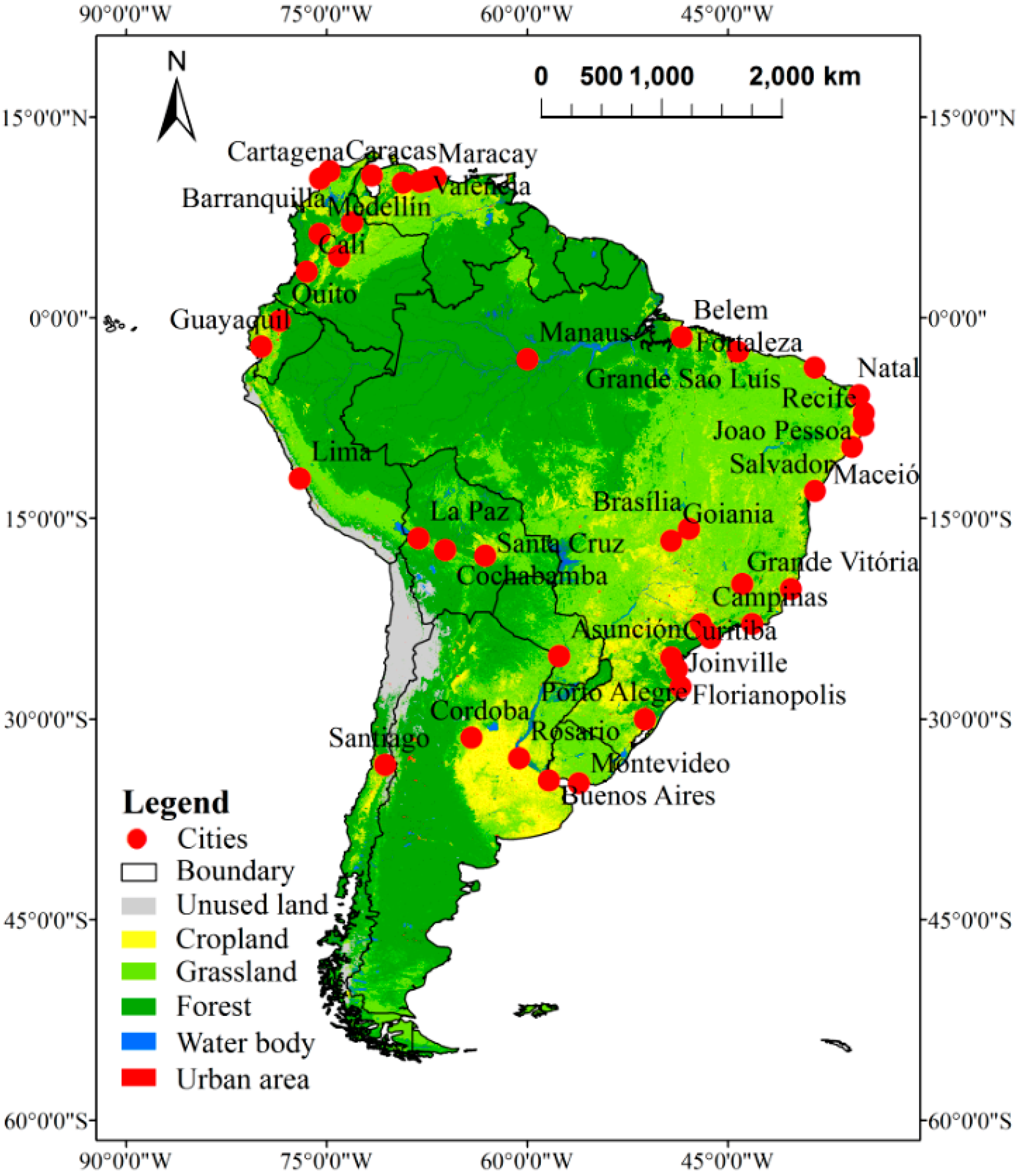
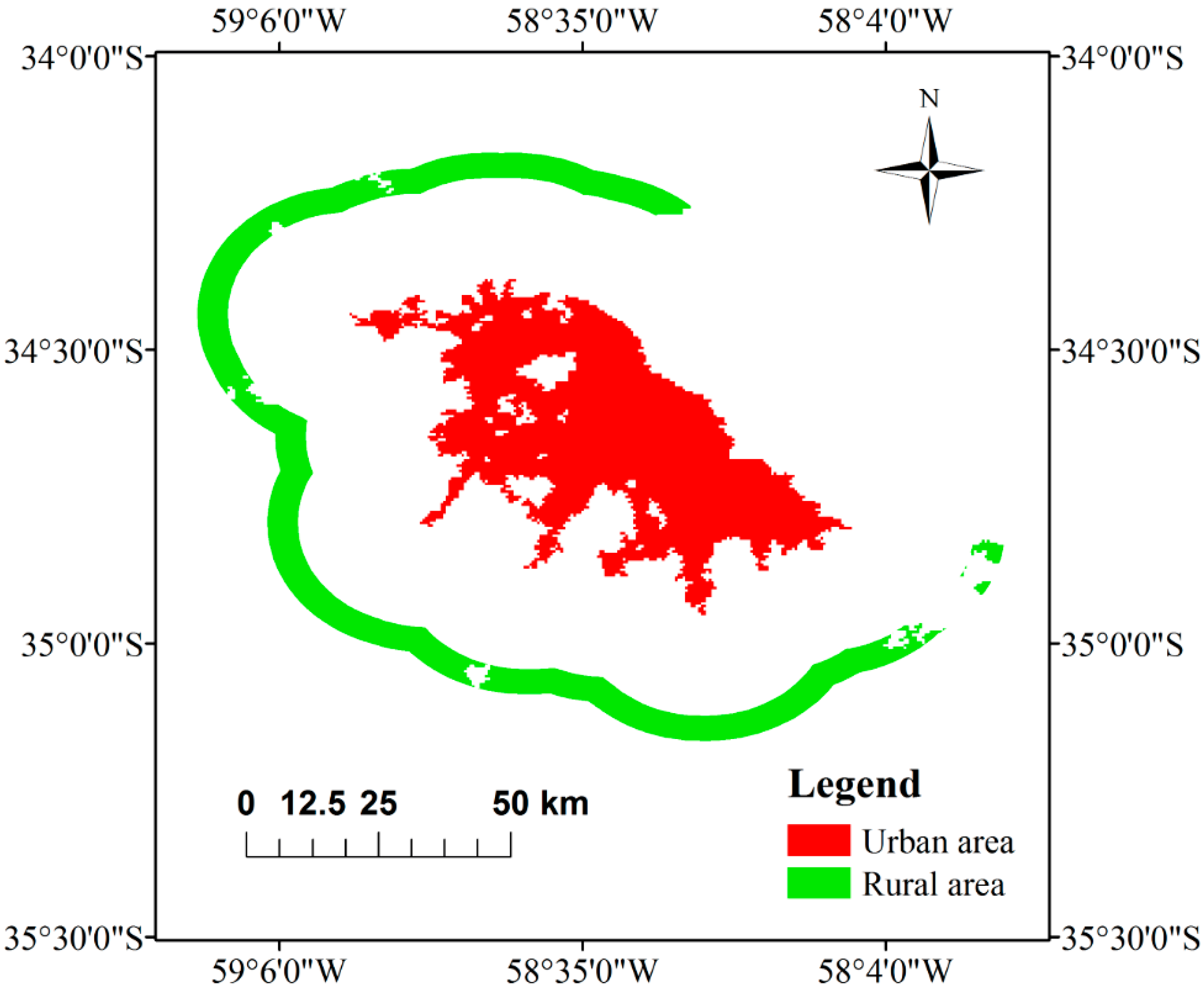
2.1. Study Area
2.2. Data
2.3. Methods
3. Results
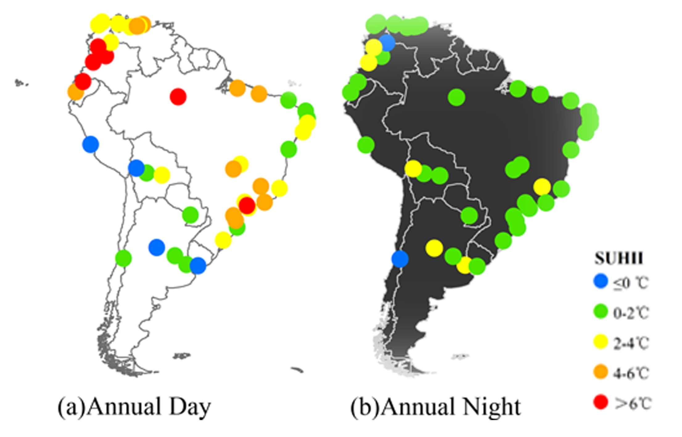
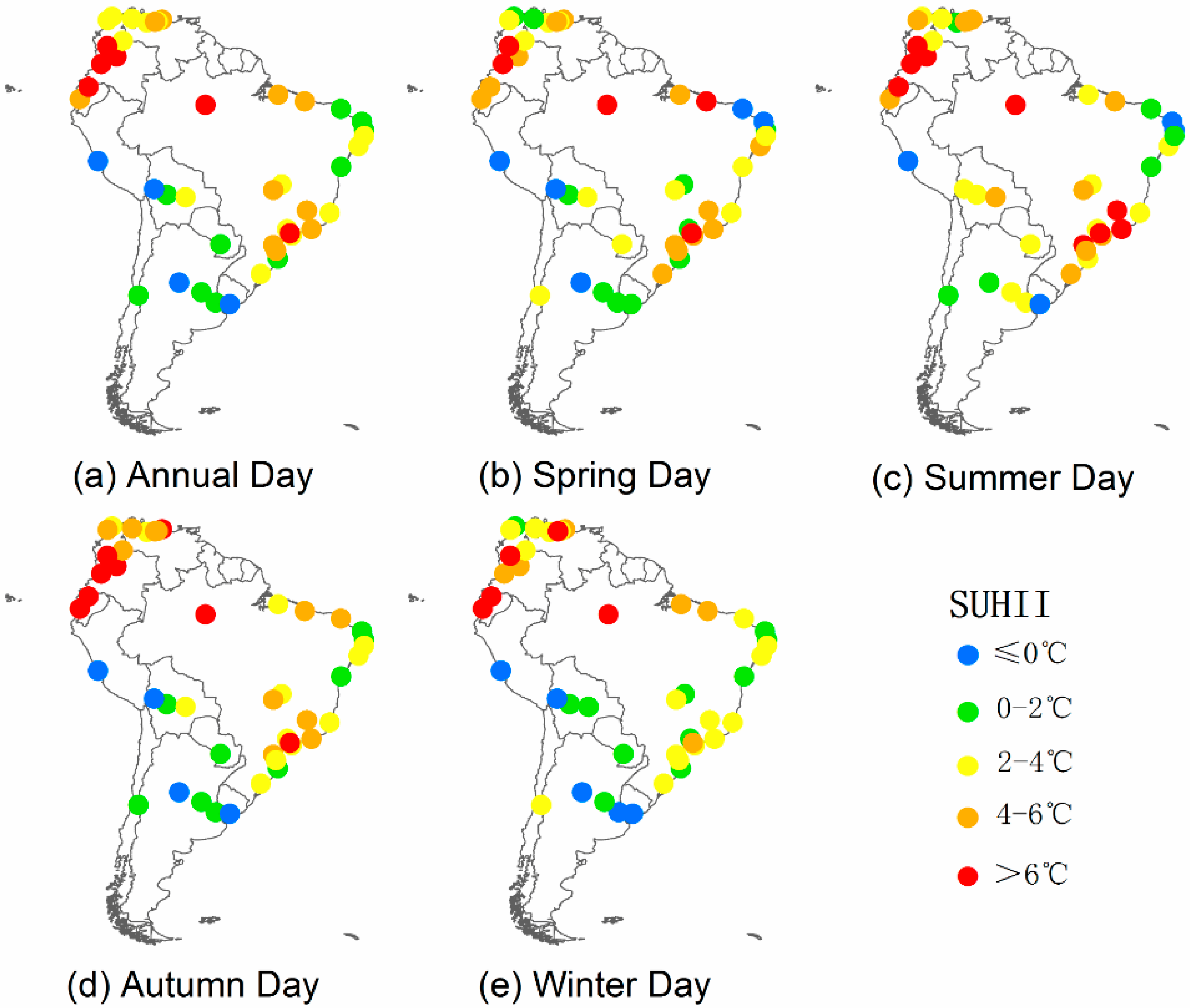
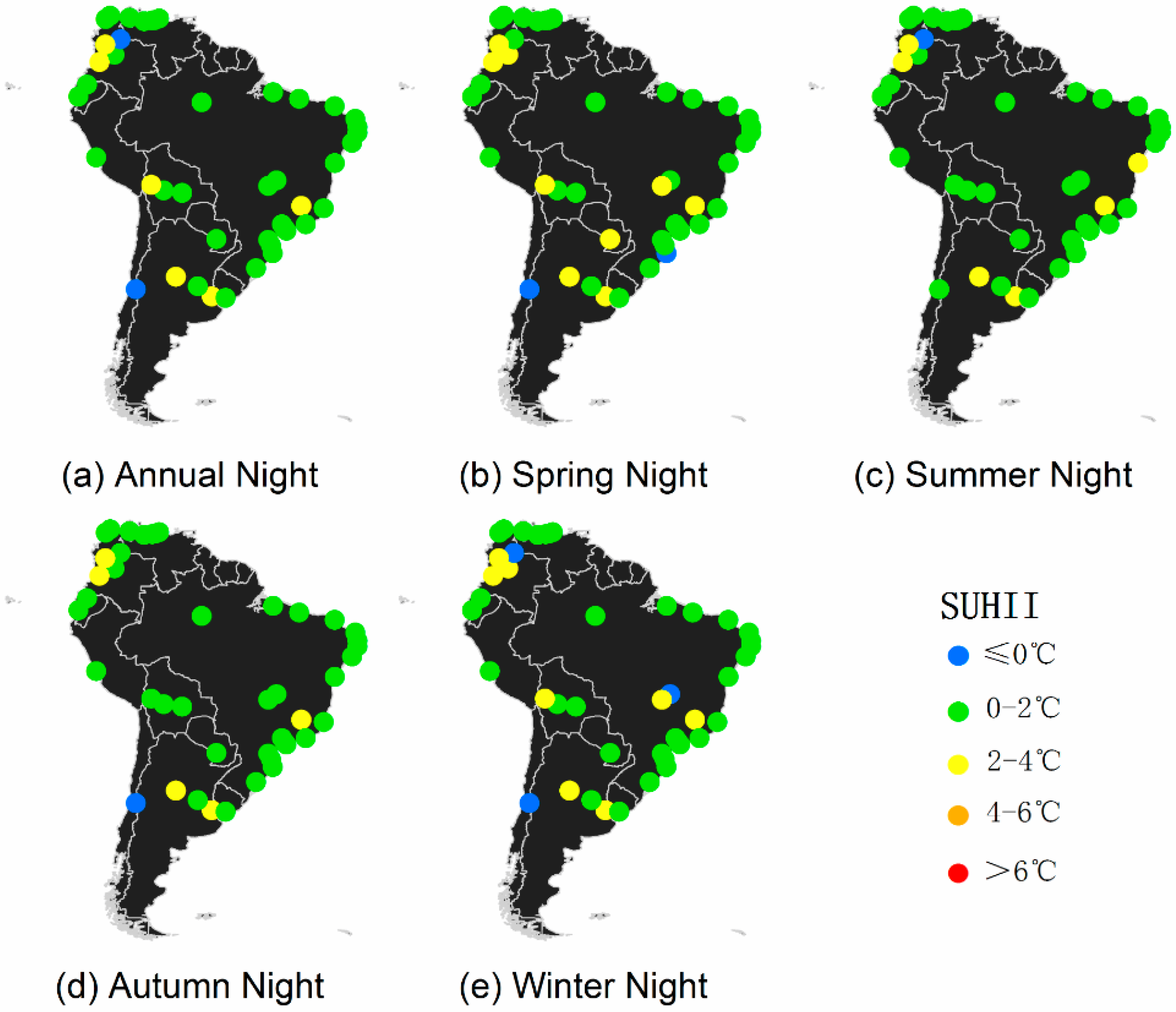
3.1. Diurnal and Seasonal Variations in the SUHII
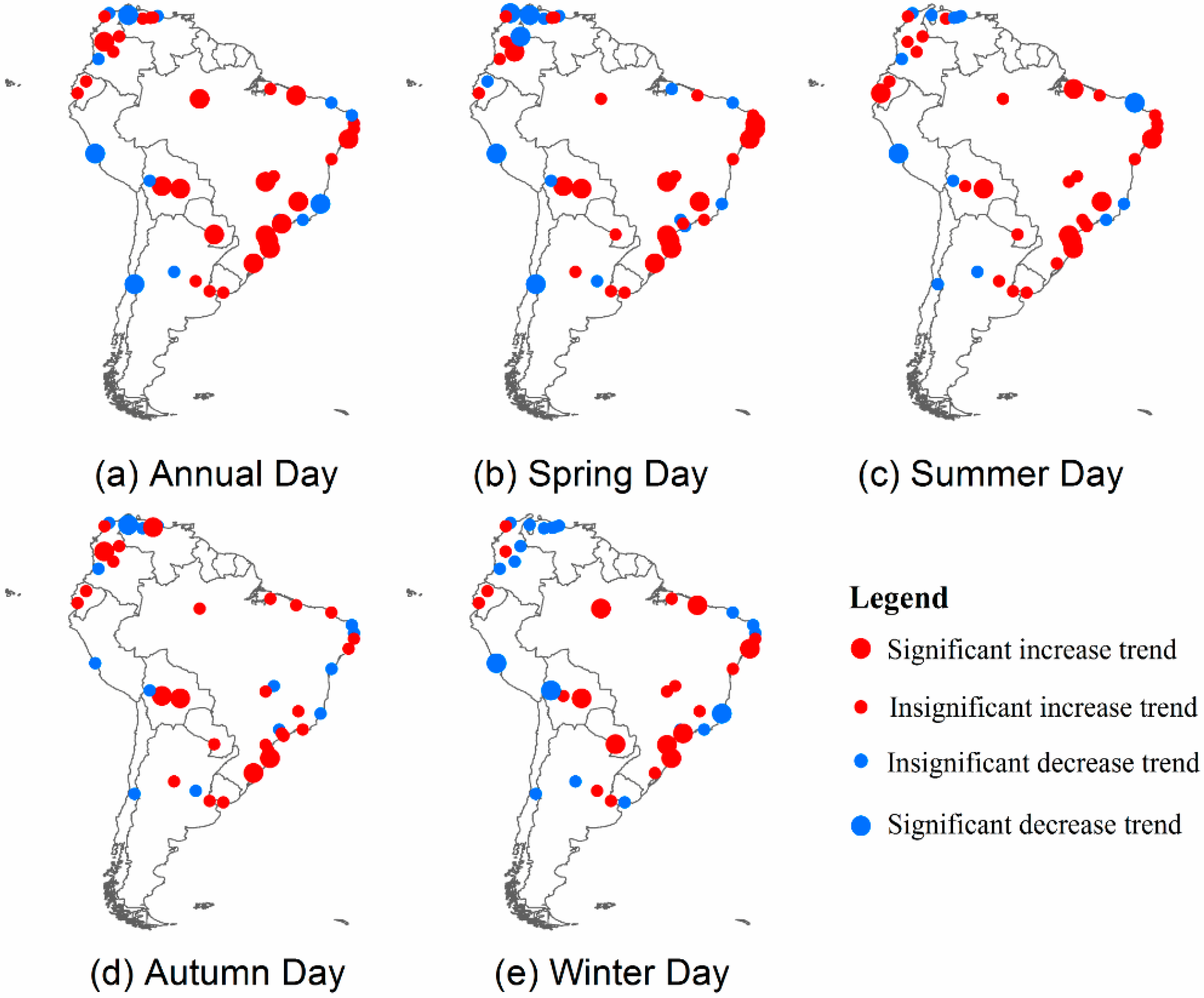
3.2. Temporal Trends in the SUHII in South America from 2003–2016
3.3. Relationships between the SUHII and Its Potential Influencing Factors
4. Discussion
4.1. Diurnal and Seasonal Variations in the SUHII
4.2. The Effects of Each Factor on SUHII
4.3. Uncertainties
5. Conclusions
Author Contributions
Funding
Acknowledgments
Conflicts of Interest
References
- United Nation. World Urbanization Prospects: The 2018 Revision; United Nation: San Francisco, CA, USA, 2017. [Google Scholar]
- Oke, T.R. The Urban Energy Balance. Prog. Phys. Geogr. 1988, 12, 471–508. [Google Scholar] [CrossRef]
- Grimm, N.B.; Faeth, S.H.; Golubiewski, N.E.; Redman, C.L.; Wu, J.G.; Bai, X.M.; Briggs, J.M. Global change and the ecology of cities. Science 2008, 319, 756–760. [Google Scholar] [CrossRef]
- Imhoff, M.L.; Bounoua, L.; DeFries, R.; Lawrence, W.T.; Stutzer, D.; Tucker, C.J.; Ricketts, T. The consequences of urban land transformation on net primary productivity in the United States. Remote Sens. Environ. 2004, 89, 434–443. [Google Scholar] [CrossRef]
- Reid, W.V. Biodiversity hotspots. Trends Ecol. Evol. 1998, 13, 275–280. [Google Scholar] [CrossRef]
- Gong, P.; Liang, S.; Carlton, E.J.; Jiang, Q.; Wu, J.; Wang, L.; Remais, J.V. Urbanisation and health in China. Lancet 2012, 379, 843–852. [Google Scholar] [CrossRef]
- O’Loughlin, J.; Witmer, F.D.; Linke, A.M.; Laing, A.; Gettelman, A.; Dudhia, J. Climate variability and conflict risk in East Africa, 1990–2009. Proc. Natl. Acad. Sci. USA 2012, 109, 18344–18349. [Google Scholar] [CrossRef]
- Patz, J.A.; Campbell-Lendrum, D.; Holloway, T.; Foley, J.A. Impact of regional climate change on human health. Nature 2005, 438, 310–317. [Google Scholar] [CrossRef]
- Arnfield, A.J. Two decades of urban climate research: A review of turbulence, exchanges of energy and water, and the urban heat island. Int. J. Climatol. 2003, 23, 1–26. [Google Scholar] [CrossRef]
- Dixon, P.G.; Mote, T.L. Patterns and causes of Atlanta’s urban heat island-initiated precipitation. J. Appl. Meteorol. 2003, 42, 1273–1284. [Google Scholar] [CrossRef]
- Jin, M.; Dickinson, R.E.; Zhang, D.A. The footprint of urban areas on global climate as characterized by MODIS. J. Clim. 2005, 18, 1551–1565. [Google Scholar] [CrossRef]
- Hung, T.; Uchihama, D.; Ochi, S.; Yasuoka, Y. Assessment with satellite data of the urban heat island effects in Asian mega cities. Int. J. Appl. Earth Obs. Geoinf. 2006, 8, 34–48. [Google Scholar]
- Jin, M.; Shepherd, J.M.; King, M.D. Urban aerosols and their variations with clouds and rainfall: A case 390 study for New York and Houston. J. Geophys. Res. Atmos. 2005. [Google Scholar] [CrossRef]
- Zhou, D.C.; Zhao, S.Q.; Liu, S.G.; Zhang, L.X.; Zhu, C. Surface urban heat island in China’s 32 major cities: Spatial patterns and drivers. Remote Sens. Environ. 2014, 152, 51–61. [Google Scholar] [CrossRef]
- Zhou, D.C.; Zhang, L.X.; Li, D.; Huang, D.; Zhu, C. Climate–vegetation control on the diurnal and seasonal variations of surface urban heat islands in China. Environ. Res. Lett. 2016, 11, 074009. [Google Scholar] [CrossRef]
- Clinton, N.; Gong, P. MODIS detected surface urban heat islands and sinks: Global locations and controls. Remote Sens. Environ. 2013, 134, 294–304. [Google Scholar] [CrossRef]
- Roth, M.; Oke, T.R.; Emery, W.J. Satellite-derived urban heat islands from three coastal cities and the utilization of such data in urban climatology. Int. J. Remote Sens. 1989, 10, 1699–1720. [Google Scholar] [CrossRef]
- Oke, T.R. Canyon geometry and the nocturnal urban heat island: Comparison of scale model and field observations. J. Climatol. 1981, 1, 237–254. [Google Scholar] [CrossRef]
- Voogt, J.A.; Oke, T.R. Thermal remote sensing of urban climates. Remote Sens. Environ. 2003, 86, 370–384. [Google Scholar] [CrossRef]
- Bonafoni, S.; Baldinelli, G.; Verducci, P.; Presciutti, A. Remote Sensing Techniques for Urban Heating Analysis: A Case Study of Sustainable Construction at District Level. Sustainability 2017, 9, 1308. [Google Scholar] [CrossRef]
- Huang, Q.; Lu, Y. Urban heat island research from 1991 to 2015: A bibliometric analysis. Theor. Appl. Climatol. 2017, 131, 1055–1067. [Google Scholar] [CrossRef]
- Tu, L.L.; Qin, Z.H.; Li, W.J.; Geng, J.; Yang, L.C.; Zhao, S.H.; Zhan, W.F.; Wang, F. Surface urban heat island effect and its relationship with urban expansion in Nanjing, China. J. Appl. Remote Sens. 2016, 10, 026037. [Google Scholar] [CrossRef]
- Zhao, M.Y.; Cai, H.Y.; Qiao, Z.; Xu, X.L. Influence of urban expansion on the urban heat island effect in Shanghai. Int. J. Geogr. Inf. Sci. 2016, 30, 2421–2441. [Google Scholar] [CrossRef]
- Parlow, E.; Vogt, R.; Feigenwinter, C. The urban heat island of Basel seen from different perspectives. J. Geogr. Soc. Berl. 2014, 145, 96–110. [Google Scholar]
- Qiao, Z.; Tian, G.; Zhang, L.; Xu, X. Influences of Urban Expansion on Urban Heat Island in Beijing during 1989–2010. Adv. Meteorol. 2014, 2014, 11. [Google Scholar] [CrossRef]
- Pongracz, R.; Bartholy, J.; Dezso, Z. Application of remotely sensed thermal information to urban climatology of Central European cities. Phys. Chem. Earth 2010, 35, 95–99. [Google Scholar] [CrossRef]
- Shastri, H.; Barik, B.; Ghosh, S.; Venkataraman, C.; Sadavarte, P. Flip flop of Day-night and Summer-Winter Surface Urban Heat Island Intensity in India. Sci. Rep. 2017, 7, 40178. [Google Scholar] [CrossRef]
- Wang, J.; Huang, B.; Fu, D.J.; Atkinson, P.M. Spatiotemporal Variation in Surface Urban Heat Island Intensity and Associated Determinants across Major Chinese Cities. Remote Sens. 2015, 7, 3670–3689. [Google Scholar] [CrossRef]
- Chakraborty, T.; Lee, X. A simplified urban-extent algorithm to characterize surface urban heat islands on a global scale and examine vegetation control on their spatiotemporal variability. Int. J. Appl. Earth Obs. Geoinf. 2019, 74, 269–280. [Google Scholar] [CrossRef]
- Yang, Q.; Huang, X.; Tang, Q. The footprint of urban heat island effect in 302 Chinese cities: Temporal trends and associated factors. Sci. Total Environ. 2019, 655, 652–662. [Google Scholar] [CrossRef]
- Weng, Q.H.; Fu, P.; Gao, F. Generating daily land surface temperature at Landsat resolution by fusing Landsat and MODIS data. Remote Sens. Environ. 2014, 145, 55–67. [Google Scholar] [CrossRef]
- Yao, R.; Wang, L.C.; Huang, X.; Niu, Z.G.; Liu, F.F.; Wang, Q. Temporal trends of surface urban heat islands and associated determinants in major Chinese cities. Sci. Total Environ. 2017, 609, 742–754. [Google Scholar] [CrossRef]
- Du, H.; Wang, D.; Wang, Y.; Zhao, X.; Qin, F.; Jiang, H.; Cai, Y. Influences of land cover types, meteorological conditions, anthropogenic heat and urban area on surface urban heat island in the Yangtze River Delta Urban Agglomeration. Sci. Total Environ. 2016, 571, 461–470. [Google Scholar] [CrossRef]
- Peng, S.S.; Piao, S.L.; Ciais, P.; Friedlingstein, P.; Ottle, C.; Breon, F.M.; Nan, H.J.; Zhou, L.M.; Myneni, R.B. Surface Urban Heat Island Across 419 Global Big Cities. Environ. Sci. Technol. 2012, 46, 696–703. [Google Scholar] [CrossRef] [PubMed]
- Weng, Q.; Lu, D.; Schubring, J. Estimation of land surface temperature–vegetation abundance relationship for urban heat island studies. Remote Sens. Environ. 2004, 89, 467–483. [Google Scholar] [CrossRef]
- Yao, R.; Wang, L.; Huang, X.; Gong, W.; Xia, X. Greening in Rural Areas Increases the Surface Urban Heat Island Intensity. Geophys. Res. Lett. 2019, 46, 2204–2212. [Google Scholar] [CrossRef]
- Wang, Y.; Berardi, U.; Akbari, H. Comparing the effects of urban heat island mitigation strategies for Toronto, Canada. Energy Build. 2016, 114, 2–19. [Google Scholar] [CrossRef]
- Fan, H.; Sailor, D. Modeling the impacts of anthropogenic heating on the urban climate of Philadelphia: A comparison of implementations in two PBL schemes. Atmos. Environ. 2005, 39, 73–84. [Google Scholar] [CrossRef]
- Palme, M.; Lobato, A.; Carrasco, C. Quantitative analysis of factors contributing to urban heat island effect in cities of latin-American Pacific coast. Procedia Eng. 2016, 169, 199–206. [Google Scholar] [CrossRef]
- Peres, L.D.; de Lucena, A.J.; Rotunno, O.C.; Franca, J.R.D. The urban heat island in Rio de Janeiro, Brazil, in the last 30 years using remote sensing data. Int. J. Appl. Earth Obs. Geoinf. 2018, 64, 104–116. [Google Scholar] [CrossRef]
- Rubel, F.; Kottek, M. Observed and projected climate shifts 1901-2100 depicted by world maps of the Köppen-Geiger climate classification. Meteorol. Z. 2010, 19, 135–141. [Google Scholar] [CrossRef]
- United Nation Population Division. Available online: https://esa.un.org/unpd/wup/DataQuery/ (accessed on 3 July 2018).
- Wan, Z.M. New refinements and validation of the MODIS Land-Surface Temperature/Emissivity products. Remote Sens. Environ. 2008, 112, 59–74. [Google Scholar] [CrossRef]
- Pablos, M.; Martinez-Fernandez, J.; Piles, M.; Sanchez, N.; Vall-Ilossera, M.; Camps, A. Multi-Temporal Evaluation of Soil Moisture and Land Surface Temperature Dynamics Using in Situ and Satellite Observations. Remote Sens. 2016, 8, 587. [Google Scholar] [CrossRef]
- Dallimer, M.; Tang, Z.; Bibby, P.R.; Brindley, P.; Gaston, K.J.; Davies, Z.G. Temporal changes in greenspace in a highly urbanized region. Biol. Lett. 2011, 7, 763–766. [Google Scholar] [CrossRef]
- Zhou, D.; Zhao, S.; Zhang, L.; Liu, S. Remotely sensed assessment of urbanization effects on vegetation phenology in China’s 32 major cities. Remote Sens. Environ. 2016, 176, 272–281. [Google Scholar] [CrossRef]
- Amaral, S.; Câmara, G.; Monteiro, A.M.V.; Quintanilha, J.A.; Elvidge, C.D. Estimating population and energy consumption in Brazilian Amazonia using DMSP night-time satellite data. Comput. Environ. Urban Syst. 2005, 29, 179–195. [Google Scholar] [CrossRef]
- Zhou, D.; Zhao, S.; Zhang, L.; Sun, G.; Liu, Y. The footprint of urban heat island effect in China. Sci. Rep. 2015, 5, 11160. [Google Scholar] [CrossRef]
- Zhang, X.; Friedl, M.A.; Schaaf, C.B.; Strahler, A.H.; Schneider, A. The footprint of urban climates on vegetation phenology. Geophys. Res. Lett. 2004. [Google Scholar] [CrossRef]
- Yao, R.; Wang, L.C.; Huang, X.; Niu, Y.; Chen, Y.S.; Niu, Z. The influence of different data and method on estimating the surface urban heat island intensity. Ecol. Indic. 2018, 89, 45–55. [Google Scholar] [CrossRef]
- Yao, R.; Wang, L.; Huang, X.; Chen, J.; Li, J.; Niu, Z. Less sensitive of urban surface to climate variability than rural in Northern China. Sci. Total Environ. 2018, 628–629, 650–660. [Google Scholar] [CrossRef]
- Kjelgren, R.; Montague, T. Urban tree transpiration over turf and asphalt surfaces. Atmos. Environ. 1998, 32, 35–41. [Google Scholar] [CrossRef]
- Han, G.; Xu, J. Land surface phenology and land surface temperature changes along an urban-rural gradient in Yangtze River Delta, China. Environ. Manag. 2013, 52, 234–249. [Google Scholar] [CrossRef]
- Hu, Y.; Jia, G. Influence of land use change on urban heat island derived from multi-sensor data. Int. J. Climatol. 2009, 30, 1382–1395. [Google Scholar] [CrossRef]
- Oke, T.R.; Cleugh, H.A.; Grimmond, C.S.B.; Schmid, H.P.; Roth, M. Evaluation of spatially-averaged fluxes of heat, mass and momentum in the urban boundary layer. Weather Clim. 1989, 9, 14–21. [Google Scholar]
- Memon, R.A.; Leung, D.Y.C.; Liu, C.H. An investigation of urban heat island intensity (UHII) as an indicator of urban heating. Atmos. Res. 2009, 94, 491–500. [Google Scholar] [CrossRef]
- Sailor, D.J. A review of methods for estimating anthropogenic heat and moisture emissions in the urban environment. Int. J. Climatol. 2011, 31, 189–199. [Google Scholar] [CrossRef]
- Ye, X.; She, B.; Benya, S. Exploring Regionalization in the Network Urban Space. J. Geovisualization Spat. Anal. 2018, 2, 4. [Google Scholar] [CrossRef]
- Rongali, G.; Keshari, A.K.; Gosain, A.K.; Khosa, R. Split-window algorithm for retrieval of land surface temperature using Landsat 8 thermal infrared data. J. Geovisualization Spat. Anal. 2018, 2, 14. [Google Scholar] [CrossRef]
- Achour, H.; Toujani, A.; Rzigui, T.; Faïz, S. Forest cover in Tunisia before and after the 2011 Tunisian revolution: A spatial analysis approach. J. Geovisualization Spat. Anal. 2018, 2, 10. [Google Scholar] [CrossRef]


| City | Country | Latitude | Longitude | Altitude (m) | Climate Zone | Type of Rural Land |
|---|---|---|---|---|---|---|
| Montevideo | Uruguay | −34.83 | −56.17 | 26.38 | Warm Temperate | Grassland |
| Buenos Aires | Argentina | −34.61 | −58.40 | 21.04 | Warm Temperate | Cropland |
| Santiago | Chile | −33.46 | −70.65 | 570.17 | Warm Temperate | Grassland |
| Rosario | Argentina | −32.95 | −60.64 | 23.47 | Warm Temperate | Cropland |
| Córdoba | Argentina | −31.41 | −64.18 | 451.06 | Warm Temperate | Cropland |
| Pôrto Alegre | Brazil | −30.03 | −51.23 | 42.95 | Warm Temperate | Grassland |
| Florianópolis | Brazil | −27.60 | −48.55 | 18.35 | Warm Temperate | Grassland |
| Joinville | Brazil | −26.30 | −48.85 | 13.28 | Warm Temperate | Forest |
| Curitiba | Brazil | −25.43 | −49.27 | 915.05 | Warm Temperate | Forest |
| Asunción | Paraguay | −25.30 | −57.64 | 110.81 | Warm Temperate | Grassland |
| Baixada Santista | Brazil | −23.96 | −46.33 | 13.69 | Warm Temperate | Forest |
| São Paulo | Brazil | −23.55 | −46.64 | 770.25 | Warm Temperate | Forest |
| Campinas | Brazil | −22.91 | −47.07 | 608.43 | Warm Temperate | Cropland |
| Rio de Janeiro | Brazil | −22.90 | −43.21 | 34.79 | Equatorial | Grassland |
| Grande Vitória | Brazil | −20.31 | −40.31 | 20.19 | Equatorial | Grassland |
| Belo Horizonte | Brazil | −19.92 | −43.94 | 870.04 | Equatorial | Grassland |
| Santa Cruz | Bolivia | −17.80 | −63.17 | 411.61 | Equatorial | Grassland |
| Cochabamba | Bolivia | −17.39 | −66.16 | 2628.62 | Warm Temperate | Grassland |
| Goiânia | Brazil | −16.68 | −49.25 | 782.09 | Equatorial | Grassland |
| La Paz | Bolivia | −16.50 | −68.15 | 3862.25 | Warm Temperate | Grassland |
| Brasília | Brazil | −15.78 | −47.93 | 1116.89 | Equatorial | Grassland |
| Salvador | Brazil | −12.97 | −38.51 | 38.42 | Equatorial | Cropland |
| Lima | Peru | −12.04 | −77.03 | 381.30 | Arid | Bare Soil |
| Maceió | Brazil | −9.67 | −35.74 | 51.37 | Equatorial | Cropland |
| Recife | Brazil | −8.05 | −34.88 | 25.47 | Equatorial | Cropland |
| João Pessoa | Brazil | −7.12 | −34.86 | 41.23 | Equatorial | Cropland |
| Natal | Brazil | −5.80 | −35.21 | 49.52 | Equatorial | Grassland |
| Fortaleza | Brazil | −3.74 | −38.54 | 19.83 | Equatorial | Grassland |
| Manaus | Brazil | −3.10 | −60.03 | 56.26 | Equatorial | Forest |
| Grande São Luís | Brazil | −2.54 | −44.28 | 30.61 | Equatorial | Grassland |
| Guayaquil | Ecuador | −2.17 | −79.90 | 12.91 | Equatorial | Grassland |
| Belém | Brazil | −1.46 | −48.48 | 19.71 | Equatorial | Forest |
| Quito | Ecuador | −0.23 | −78.52 | 2766.80 | Warm Temperate | Grassland |
| Cali | Colombia | 3.44 | −76.52 | 989.71 | Equatorial | Cropland |
| Bogotá | Colombia | 4.61 | −74.08 | 2591.86 | Warm Temperate | Grassland |
| Medellín | Colombia | 6.25 | −75.56 | 1602.91 | Equatorial | Forest |
| Bucaramanga | Colombia | 7.13 | −73.12 | 857.72 | Equatorial | Forest |
| Barquisimeto | Venezuela | 10.07 | −69.32 | 600.40 | Equatorial | Grassland |
| Valencia | Venezuela | 10.16 | −68.01 | 473.51 | Equatorial | Grassland |
| Maracay | Venezuela | 10.25 | −67.60 | 456.26 | Equatorial | Grassland |
| Cartagena | Colombia | 10.40 | −75.51 | 10.98 | Equatorial | Grassland |
| Caracas | Venezuela | 10.49 | −66.88 | 965.61 | Equatorial | Forest |
| Maracaibo | Venezuela | 10.63 | −71.64 | 23.98 | Equatorial | Grassland |
| Barranquilla | Colombia | 10.96 | −74.80 | 35.72 | Equatorial | Grassland |
| Climate Zone | Spring | Summer | Autumn | Winter | Annual | |
|---|---|---|---|---|---|---|
| Daytime | Equatorial | 3.45 | 3.93 | 4.16 | 3.61 | 3.80 |
| Arid | −2.84 | −1.45 | −0.67 | −1.41 | −1.60 | |
| Warm temperate | 2.67 | 4.06 | 2.62 | 1.77 | 2.77 | |
| Night-time | Equatorial | 1.32 | 1.22 | 1.15 | 1.18 | 1.22 |
| Arid | 0.93 | 0.94 | 1.15 | 0.88 | 1.03 | |
| Warm temperate | 1.44 | 1.43 | 1.30 | 1.17 | 1.34 |
| Type of Rural Land | Spring | Summer | Autumn | Winter | Annual | |
|---|---|---|---|---|---|---|
| Daytime | Forest | 5.58 | 6.05 | 5.32 | 4.92 | 5.47 |
| Cropland | 1.96 | 2.60 | 2.09 | 1.59 | 2.06 | |
| Grassland | 2.59 | 3.72 | 3.49 | 2.55 | 3.09 | |
| Bare soil | −6.63 | −6.46 | −6.51 | −5.02 | −6.16 | |
| Night-time | Forest | 1.29 | 1.11 | 1.11 | 1.02 | 1.13 |
| Cropland | 1.85 | 1.85 | 1.60 | 1.54 | 1.71 | |
| Grassland | 1.20 | 1.17 | 1.11 | 1.10 | 1.15 | |
| Bare soil | 0.99 | 0.78 | 1.01 | 0.60 | 0.85 |
| Factors | Daytime | Night-time | ||||||
|---|---|---|---|---|---|---|---|---|
| Spring | Summer | Autumn | Winter | Spring | Summer | Autumn | Winter | |
| ∆EVI | −0.81 a | −0.79 a | −0.78 a | −0.80 a | −0.16 | −0.25 | −0.30 | −0.18 |
| Urban area | 0.04 | 0.14 | −0.04 | −0.10 | 0.20 | 0.36b | 0.25 | 0.13 |
| Population | 0.08 | 0.12 | −0.01 | −0.01 | 0.15 | 0.29 | 0.20 | 0.10 |
| Altitude | 0.17 | 0.24 | 0.20 | 0.13 | 0.02 | −0.08 | −0.02 | 0.01 |
| ∆NL | 0.21 | 0.31 | 0.22 | 0.12 | 0.31 | 0.63a | 0.46 b | 0.51a |
| Spring | Summer | Autumn | Winter | Annual Average | |
|---|---|---|---|---|---|
| Daytime | 2.86 | 3.74 | 3.34 | 2.67 | 3.15 |
| Night-time | 1.34 | 1.28 | 1.21 | 1.16 | 1.25 |
| Spring | Summer | Autumn | Winter | Annual | |
|---|---|---|---|---|---|
| Rural EVI | |||||
| Six cities | 0.43 | 0.46 | 0.44 | 0.43 | 0.44 |
| Equatorial cities | 0.36 | 0.43 | 0.45 | 0.39 | 0.41 |
| Warm temperate cities | 0.32 | 0.42 | 0.38 | 0.30 | 0.36 |
| Arid cities | 0.06 | 0.06 | 0.05 | 0.06 | 0.06 |
| ∆EVI | |||||
| Six cities | −0.19 | −0.20 | −0.19 | −0.19 | −0.20 |
| Equatorial cities | −0.12 | −0.15 | −0.16 | −0.14 | −0.14 |
| Warm temperate cities | −0.09 | −0.13 | −0.12 | −0.10 | −0.11 |
| Arid cities | 0.01 | 0.01 | 0.02 | 0.00 | 0.01 |
© 2019 by the authors. Licensee MDPI, Basel, Switzerland. This article is an open access article distributed under the terms and conditions of the Creative Commons Attribution (CC BY) license (http://creativecommons.org/licenses/by/4.0/).
Share and Cite
Wu, X.; Wang, G.; Yao, R.; Wang, L.; Yu, D.; Gui, X. Investigating Surface Urban Heat Islands in South America Based on MODIS Data from 2003–2016. Remote Sens. 2019, 11, 1212. https://doi.org/10.3390/rs11101212
Wu X, Wang G, Yao R, Wang L, Yu D, Gui X. Investigating Surface Urban Heat Islands in South America Based on MODIS Data from 2003–2016. Remote Sensing. 2019; 11(10):1212. https://doi.org/10.3390/rs11101212
Chicago/Turabian StyleWu, Xiaojun, Guangxing Wang, Rui Yao, Lunche Wang, Deqing Yu, and Xuan Gui. 2019. "Investigating Surface Urban Heat Islands in South America Based on MODIS Data from 2003–2016" Remote Sensing 11, no. 10: 1212. https://doi.org/10.3390/rs11101212
APA StyleWu, X., Wang, G., Yao, R., Wang, L., Yu, D., & Gui, X. (2019). Investigating Surface Urban Heat Islands in South America Based on MODIS Data from 2003–2016. Remote Sensing, 11(10), 1212. https://doi.org/10.3390/rs11101212