An Improved Ball Pivot Algorithm-Based Ground Filtering Mechanism for LiDAR Data


Abstract
1. Introduction
2. Methods
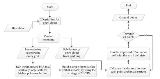
2.1. Overview
2.2. BPA and Its Limitation for Point Cloud Filtering
2.3. Improved Ball Pivoting Algorithm Based on Spatial Sorting
| Algorithm 1: the improved ball-pivoting algorithm for ground point filtering |
| Input: A set of points . Output: ground points and none-ground points . While is not empty:
|
3. Area of Interest and Data Set
4. Experimental Results and Discussion
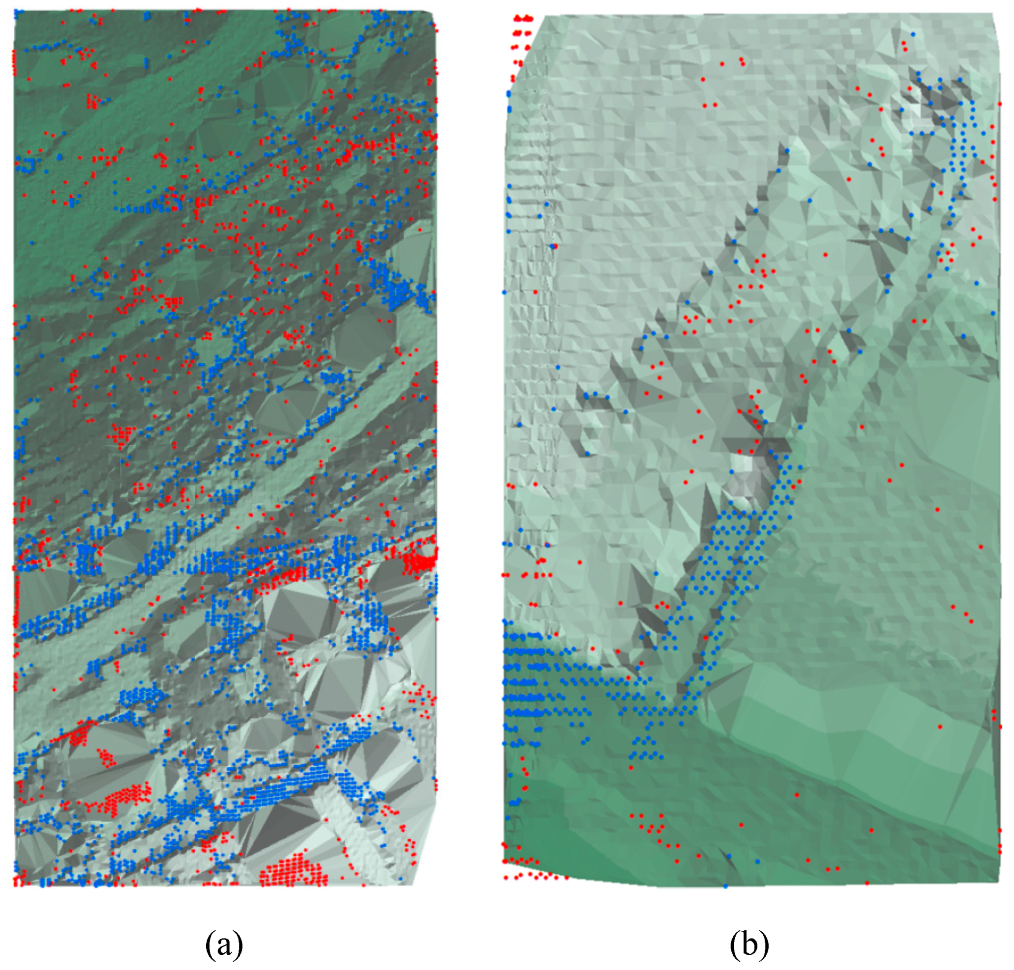
4.1. Experimental Results
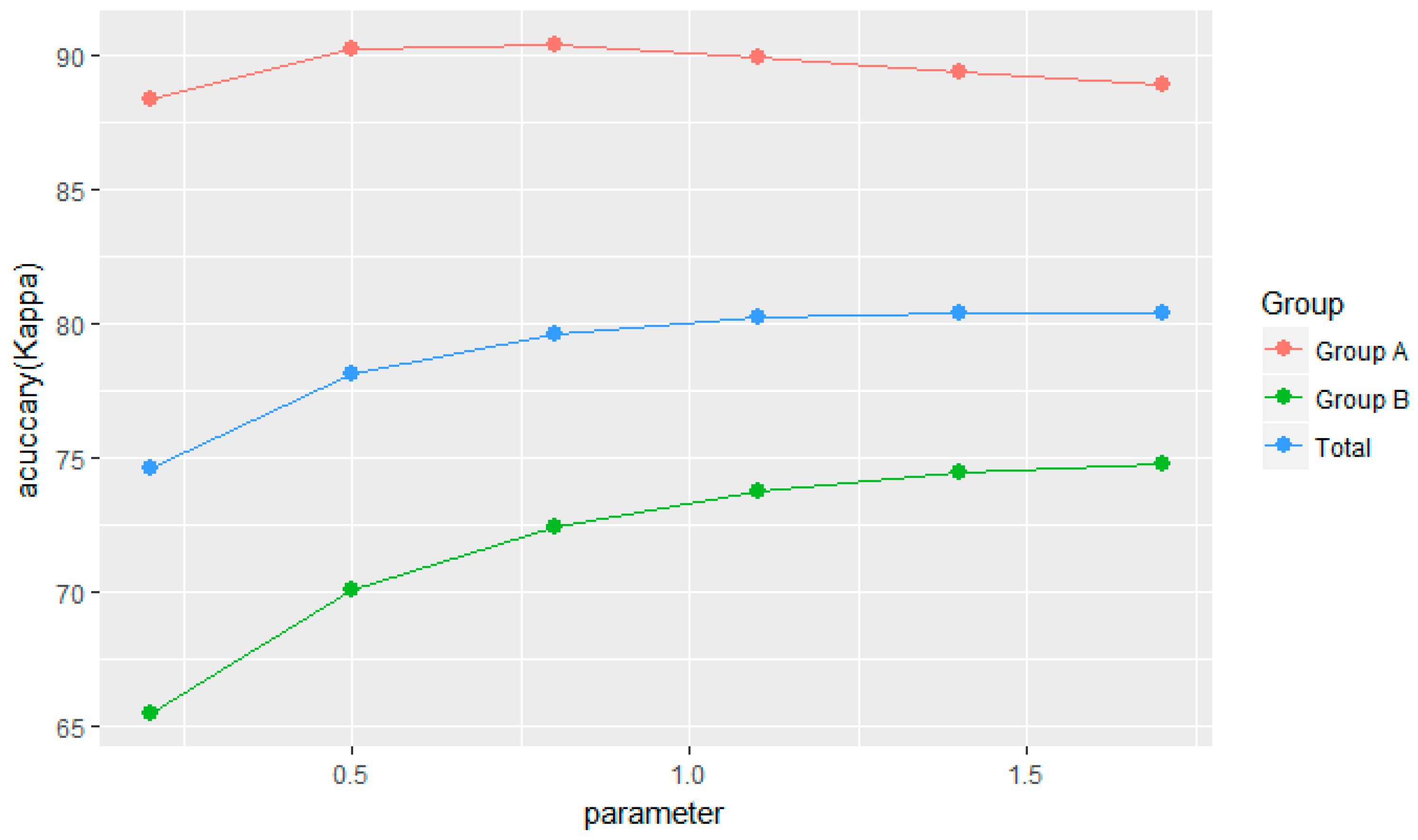
4.2. Discussion
5. Conclusions and Future Work
Author Contributions
Funding
Acknowledgments
Conflicts of Interest
References
- Sheng, N.; Cheng, W.; Dong, P.; Xi, X.; Luo, S.; Qin, H. A revised progressive TIN densification for filtering airborne LiDAR data. Measurement 2017, 104, 70–77. [Google Scholar]
- Zhang, J.; Lin, X. Filtering airborne LiDAR data by embedding smoothness-constrained segmentation in progressive TIN densification. ISPRS J. Photogramm. Remote Sens. 2013, 81, 44–59. [Google Scholar] [CrossRef]
- Hu, H.; Ding, Y.; Zhu, Q.; Wu, B.; Lin, H.; Du, Z.; Zhang, Y.; Zhang, Y. An adaptive surface filter for airborne laser scanning point clouds by means of regularization and bending energy. ISPRS J. Photogramm. Remote Sens. 2014, 92, 98–111. [Google Scholar] [CrossRef]
- Chen, Y.; Jiang, H.; Li, C.; Jia, X.; Ghamisi, P. Deep Feature Extraction and Classification of Hyperspectral Images Based on Convolutional Neural Networks. IEEE Trans. Geosci. Remote Sens. 2016, 54, 6232–6251. [Google Scholar] [CrossRef]
- Chen, Z.; Gao, B.; Devereux, B. State-of-the-Art: DTM Generation Using Airborne LIDAR Data. Sensors 2017, 17, 150. [Google Scholar] [CrossRef]
- Mou, L.; Bruzzone, L.; Xiao, X.Z. Learning Spectral-Spatial-Temporal Features via a Recurrent Convolutional Neural Network for Change Detection in Multispectral Imagery. IEEE Trans. Geosci. Remote Sens. 2018, 57, 1–12. [Google Scholar] [CrossRef]
- Ghamisi, P.; Chen, Y.; Xiao, X.Z. A Self-Improving Convolution Neural Network for the Classification of Hyperspectral Data. IEEE Geosci. Remote Sens. Lett. 2017, 13, 1537–1541. [Google Scholar] [CrossRef]
- Hughes, L.H.; Schmitt, M.; Mou, L.C.; Wang, Y.; Zhu, X. Identifying Corresponding Patches in SAR and Optical Images with a Pseudo-Siamese CNN. IEEE Geosci. Remote Sens. Lett. 2017, 15, 1–5. [Google Scholar] [CrossRef]
- Chen, C.; Li, Y.; Wei, L.; Dai, H. A multiresolution hierarchical classification algorithm for filtering airborne LiDAR data. ISPRS J. Photogramm. Remote Sens. 2013, 82, 1–9. [Google Scholar] [CrossRef]
- Hu, X.; Yuan, Y. Deep-Learning-Based Classification for DTM Extraction from ALS Point Cloud. Remote Sens. 2016, 8, 730. [Google Scholar] [CrossRef]
- Mou, L.; Ghamisi, P.; Zhu, X. Unsupervised Spectral-Spatial Feature Learning via Deep Residual Conv-Deconv Network for Hyperspectral Image Classification. IEEE Trans. Geosci. Remote Sens. 2018, 56, 1–16. [Google Scholar] [CrossRef]
- Lin, Z.; Chen, Y.; Ghamisi, P.; Benediktsson, J.A. Generative Adversarial Networks for Hyperspectral Image Classification. IEEE Trans. Geosci. Remote Sens. 2018, 56, 1–18. [Google Scholar]
- Axelsson, P. DEM Generation from Laser Scanner Data Using Adaptive TIN Models. Int. Arch. Photogramm. Remote Sens. Spatial Inf. Sci. 2000, 33, 110–117. [Google Scholar]
- Zhao, X.; Guo, Q.; Su, Y.; Xue, B. Improved progressive TIN densification filtering algorithm for airborne LiDAR data in forested areas. ISPRS J. Photogramm. Remote Sens. 2016, 117, 79–91. [Google Scholar] [CrossRef]
- Sohn, G.; Dowman, I. Terrain surface reconstruction by the use of tetrahedron model with the MDL criterion. Int. Arch. Photogramm. Remote Sens. Spatial Inf. Sci. 2002, 34, 336–344. [Google Scholar]
- Sithole, G.; Vosselman, G. Experimental comparison of filter algorithms for bare-Earth extraction from airborne laser scanning point clouds ☆. ISPRS J. Photogramm. Remote Sens. 2004, 59, 85–101. [Google Scholar] [CrossRef]
- Axelsson, P. Processing of laser scanner data—algorithms and applications. ISPRS J. Photogramm. Remote Sens. 1999, 54, 138–147. [Google Scholar] [CrossRef]
- Lin, X.; Zhang, J. Segmentation-Based Filtering of Airborne LiDAR Point Clouds by Progressive Densification of Terrain Segments. Remote Sens. 2014, 6, 1294–1326. [Google Scholar] [CrossRef]
- Quan, Y.; Song, J.; Xue, G.; Miao, Q.; Yun, Y. Filtering LiDAR data based on adjacent triangle of triangulated irregular network. Multimed. Tools Appl. 2016, 76, 1–13. [Google Scholar] [CrossRef]
- Zhe, Z.; Wan, J.; Hui, L. An entropy-based filtering approach for airborne laser scanning data. Infrared Phys. Technol. 2016, 75, 87–92. [Google Scholar]
- Kilian, J.; Haala, N.; Englich, M. Capture and evaluation of airborne laser scanner data. ISPRS Photogramm. Remote Sens. Spatial Inf. Sci. 1996, 31, 383–388. [Google Scholar]
- Zhang, K.; Whitman, D. Comparison of Three Algorithms for Filtering Airborne Lidar Data. Photogramm. Eng. Remote Sens. 2005, 71, 313–324. [Google Scholar] [CrossRef]
- Yong, L.; Yong, B.; Wu, H.; Ru, A.; Xu, H. An Improved Top-Hat Filter with Sloped Brim for Extracting Ground Points from Airborne Lidar Point Clouds. Remote Sens. 2014, 6, 12885–12908. [Google Scholar]
- Susaki, J. Adaptive Slope Filtering of Airborne LiDAR Data in Urban Areas for Digital Terrain Model (DTM) Generation. Remote Sens. 2012, 4, 1804–1819. [Google Scholar] [CrossRef]
- Mongus, D.; Žalik, B. Parameter-free ground filtering of LiDAR data for automatic DTM generation. ISPRS J. Photogramm. Remote Sens. 2012, 67, 1–12. [Google Scholar] [CrossRef]
- Mongus, D.; Lukač, N.; Žalik, B. Ground and building extraction from LiDAR data based on differential morphological profiles and locally fitted surfaces. ISPRS J. Photogramm. Remote Sens. 2014, 93, 145–156. [Google Scholar] [CrossRef]
- Hui, Z.; Hu, Y.; Yao, Z.Y.; Yu, X. An Improved Morphological Algorithm for Filtering Airborne LiDAR Point Cloud Based on Multi-Level Kriging Interpolation. Remote Sens. 2016, 8, 35. [Google Scholar] [CrossRef]
- Qi, C.; Peng, G.; Baldocchi, D.; Xie, G. Filtering Airborne Laser Scanning Data with Morphological Methods. Photogramm. Eng. Remote Sens. 2007, 73, 175–185. [Google Scholar]
- Evans, J.S.; Hudak, A.T. A multiscale curvature algorithm for classifying discrete return LiDAR in forested environments. IEEE Trans. Geosci. Remote Sens. 2007, 45, 1029–1038. [Google Scholar] [CrossRef]
- Lee, H.S.; Younan, N.H. DTM extraction of LiDAR returns via adaptive processing. IEEE Trans. Geosci. Remote Sens. 2003, 41, 2063–2069. [Google Scholar] [CrossRef]
- Zhang, W.; Qi, J.; Peng, W.; Wang, H.; Xie, D.; Wang, X.; Yan, G. An Easy-to-Use Airborne LiDAR Data Filtering Method Based on Cloth Simulation. Remote Sens. 2016, 8, 501. [Google Scholar] [CrossRef]
- Wang, L.; Xu, Y.; Li, Y. Aerial Lidar Point Cloud Voxelization with its 3D Ground Filtering Application. Photogramm. Eng. Remote Sens. 2017, 83, 95–107. [Google Scholar] [CrossRef]
- Edelsbrunner, H.; Kirkpatrick, D.; Seidel, R. On the Shape of a Set of Points in the Plane. IEEE Trans. Inf. Theory 1983, 29, 551–559. [Google Scholar] [CrossRef]
- Edelsbrunner, H.; Mücke, E.P. Three-dimensional Alpha Shapes. Acm Trans. Graph. 1994, 13, 43–72. [Google Scholar] [CrossRef]
- Bernardini, F.M.J.; Rushmeier, H. The ball-pivoting algorithm for surface reconstruction. IEEE Trans. Vis. Comput. Graph. 2002, 5, 349–359. [Google Scholar] [CrossRef]
- Edelsbrunner, H. Tessellations in the Sciences; Virtues, Techniques and Applications of Geometric Tilings. In Alpha Shapes—A Survey; Springer: Heidelberg, Germany, 2010. [Google Scholar]
- Demir, N. Use of Airborne Laser Scanning Data and Image-based Three-dimensional (3-D) Edges for Automated Planar Roof Reconstruction. Lasers Eng. (Old City Publ.) 2015, 32, 173–205. [Google Scholar]
- Paavo, N.; Maarit, M.; Raimo, S.; Jukka, H.; Tapio, P. Detecting Terrain Stoniness From Airborne Laser Scanning Data. Remote Sens. 2016, 8, 720. [Google Scholar] [CrossRef]
- Wu, B.; Yu, B.; Chang, H.; Wu, Q.; Wu, J. Automated extraction of ground surface along urban roads from mobile laser scanning point clouds. Remote Sens. Lett. 2016, 7, 170–179. [Google Scholar] [CrossRef]
- Digne, J. An Analysis and Implementation of a Parallel Ball Pivoting Algorithm. Image Process. Line 2014, 4, 149–168. [Google Scholar] [CrossRef]
- Dong, C.; Zhang, L.Q.; Zhen, W.; Hao, D. A mathematical morphology-based multi-level filter of LiDAR data for generating DTMs. Sci. China Inf. Sci. 2013, 56, 1–14. [Google Scholar]
- Yong, L.; Wu, H.; Xu, H.; Ru, A.; Jia, X.; He, Q. A gradient-constrained morphological filtering algorithm for airborne LiDAR. Opt. Laser Technol. 2013, 54, 288–296. [Google Scholar]
- Jahromi, A.B.; Zoej, M.J.V.; Mohammadzadeh, A.; Sadeghian, S. A Novel Filtering Algorithm for Bare-Earth Extraction from Airborne Laser Scanning Data Using an Artificial Neural Network. IEEE J. Sel. Top. Appl. Earth Obs. Remote Sens. 2011, 4, 836–843. [Google Scholar] [CrossRef]
- Pingel, T.J.; Clarke, K.C.; Mcbride, W.A. An improved simple morphological filter for the terrain classification of airborne LIDAR data. ISPRS J. Photogramm. Remote Sens. 2013, 77, 21–30. [Google Scholar] [CrossRef]


| Group | Feature | Samples |
|---|---|---|
| A | Flat terrain or gentle slope, few steep slopes | 12,21,31,42,51,54 |
| B | With steep or terraced slopes (e.g., river bank, ditch, terrace, pit, cliff) | 11,22,23,24,41,52,53,61,71 |
| Sample | |||||||
|---|---|---|---|---|---|---|---|
| Total Errors(%) | Kappa(%) | Total Errors(%) | Kappa(%) | Total Errors(%) | Kappa(%) | ||
| 2.5 | 11 | 13.96 | 72.08 | 13.95 | 72.12 | 14.66 | 70.81 |
| 12 | 4.43 | 91.14 | 4.57 | 90.86 | 4.48 | 91.04 | |
| 21 | 4.32 | 87.83 | 4.29 | 87.98 | 4.30 | 87.92 | |
| 22 | 13.53 | 67.87 | 8.50 | 80.96 | 7.41 | 83.37 | |
| 23 | 11.13 | 77.82 | 10.29 | 79.49 | 10.18 | 79.72 | |
| 24 | 10.26 | 75.66 | 10.77 | 74.91 | 10.89 | 74.61 | |
| 31 | 5.95 | 87.94 | 4.23 | 91.44 | 3.52 | 92.89 | |
| 41 | 8.52 | 82.95 | 8.25 | 83.49 | 9.03 | 81.94 | |
| 42 | 4.04 | 90.38 | 2.74 | 93.37 | 2.78 | 93.26 | |
| 5 | 51 | 3.41 | 89.62 | 3.28 | 90.00 | 3.38 | 89.71 |
| 52 | 6.64 | 68.99 | 6.38 | 70.35 | 6.58 | 69.46 | |
| 53 | 10.91 | 34.78 | 11.68 | 33.20 | 13.07 | 30.30 | |
| 54 | 6.28 | 87.44 | 6.10 | 87.81 | 6.33 | 87.35 | |
| 61 | 4.27 | 58.18 | 4.58 | 56.22 | 4.79 | 55.22 | |
| 71 | 4.59 | 78.13 | 4.44 | 79.35 | 4.74 | 78.61 | |
| Mean | 7.48 | 76.72 | 6.94 | 78.10 | 7.08 | 77.75 | |
| Min | 3.41 | 34.78 | 2.74 | 33.20 | 2.78 | 30.30 | |
| Max | 13.96 | 91.14 | 13.95 | 93.37 | 14.66 | 93.26 | |
| Std | 3.50 | 14.68 | 3.32 | 15.38 | 3.58 | 16.18 | |
| Sample | φ = 0.2 Kappa(%) | φ = 0.5 Kappa(%) | φ = 0.8 Kappa(%) | φ = 1.1 Kappa(%) | φ = 1.4 Kappa(%) | φ = 1.7 Kappa(%) | |
|---|---|---|---|---|---|---|---|
| 2.5 | 11 | 67.45 | 72.12 | 74.08 | 74.73 | 74.86 | 74.21 |
| 12 | 87.91 | 90.86 | 91. 06 | 91.02 | 90.38 | 90.16 | |
| 21 | 84.54 | 87.98 | 89.50 | 89.10 | 88.63 | 88.37 | |
| 22 | 77.47 | 80.96 | 81.82 | 82.77 | 83.26 | 83.44 | |
| 23 | 75.90 | 79.49 | 81.49 | 82.44 | 83.49 | 83.93 | |
| 24 | 72.37 | 74.91 | 74.86 | 74.88 | 75.10 | 75.25 | |
| 31 | 91.02 | 91.44 | 90.28 | 89.10 | 88.36 | 87.42 | |
| 41 | 81.06 | 83.49 | 84.91 | 86.82 | 87.35 | 87.44 | |
| 42 | 91.61 | 93.37 | 93.88 | 93.50 | 92.81 | 92.15 | |
| 5 | 51 | 87.69 | 90.00 | 89.97 | 89.78 | 89.43 | 88.92 |
| 52 | 64.49 | 70.35 | 72.47 | 73.79 | 74.31 | 74.18 | |
| 53 | 29.38 | 33.20 | 35.76 | 37.49 | 39.02 | 40.26 | |
| 54 | 87.47 | 87.81 | 87.63 | 86.93 | 86.47 | 86.16 | |
| 61 | 50.35 | 56.22 | 61.76 | 64.99 | 66.98 | 68.05 | |
| 71 | 70.26 | 79.35 | 84.61 | 85.47 | 85.32 | 85.63 | |
| Mean | 74.60 | 78.10 | 79.61 | 80.19 | 80.38 | 80.37 | |
| Min | 29.38 | 33.20 | 35.76 | 37.49 | 39.02 | 40.26 | |
| Max | 91.61 | 93.37 | 93.88 | 93.50 | 92.81 | 92.15 | |
| Std | 16.40 | 15.38 | 14.43 | 13.73 | 13.12 | 12.70 |
| Sample | φ = 0.2 Total Errors(%) | φ = 0.5 Total Errors(%) | φ = 0.8 Total Errors(%) | φ = 1.1 Total Errors(%) | φ = 1.4 Total Errors(%) | φ = 1.7 Total Errors(%) | |
|---|---|---|---|---|---|---|---|
| 2.5 | 11 | 17.73 | 13.95 | 13.33 | 12.50 | 12.38 | 12.66 |
| 12 | 6.05 | 4.57 | 4.69 | 4.49 | 4.81 | 4.93 | |
| 21 | 5.65 | 4.29 | 3.67 | 3.79 | 3.94 | 4.03 | |
| 22 | 10.68 | 8.50 | 8.26 | 7.54 | 7.31 | 7.11 | |
| 23 | 13.97 | 10.29 | 10.28 | 8.79 | 8.86 | 8.51 | |
| 24 | 12.09 | 10.77 | 10.69 | 10.50 | 10.33 | 10.17 | |
| 31 | 4.97 | 4.23 | 4.89 | 5.38 | 5.77 | 6.21 | |
| 41 | 10.04 | 8.25 | 7.72 | 6.59 | 6.49 | 6.45 | |
| 42 | 3.43 | 2.74 | 2.54 | 2.72 | 3.01 | 3.30 | |
| 5 | 51 | 5.18 | 3.28 | 3.27 | 3.32 | 3.86 | 4.04 |
| 52 | 8.16 | 6.38 | 5.59 | 5.35 | 5.24 | 5.15 | |
| 53 | 14.45 | 11.68 | 10.96 | 9.75 | 9.46 | 9.00 | |
| 54 | 6.24 | 6.10 | 6.18 | 6.55 | 6.57 | 6.73 | |
| 61 | 6.19 | 4.58 | 3.96 | 3.20 | 3.12 | 2.92 | |
| 71 | 7.00 | 4.44 | 3.11 | 2.87 | 2.85 | 2.76 | |
| Mean | 8.79 | 6.94 | 6.61 | 6.22 | 6.27 | 6.26 | |
| Min | 3.43 | 2.74 | 2.54 | 2.72 | 3.01 | 3.30 | |
| Max | 17.73 | 13.95 | 13.33 | 12.50 | 12.92 | 12.92 | |
| Std | 4.19 | 3.32 | 3.40 | 2.95 | 2.91 | 2.86 |
| Sample | Type I(%) | Type II(%) | Total Errors(%) | Kappa(%) | |
|---|---|---|---|---|---|
| 2.5 | 11 | 14.17 | 10.26 | 12.50 | 74.73 |
| 12 | 3.81 | 5.20 | 4.49 | 91.02 | |
| 21 | 2.71 | 7.58 | 3.79 | 89.10 | |
| 22 | 7.07 | 8.57 | 7.54 | 82.77 | |
| 23 | 11.74 | 5.50 | 8.79 | 82.44 | |
| 24 | 10.25 | 11.18 | 10.50 | 74.88 | |
| 31 | 7.20 | 10.82 | 5.38 | 89.10 | |
| 41 | 9.62 | 3.57 | 6.59 | 86.82 | |
| 42 | 3.05 | 2.58 | 2.72 | 93.50 | |
| 5 | 51 | 0.30 | 14.15 | 3.32 | 89.78 |
| 52 | 4.13 | 15.75 | 5.35 | 73.79 | |
| 53 | 9.53 | 15.05 | 9.75 | 37.49 | |
| 54 | 1.10 | 11.24 | 6.55 | 86.93 | |
| 61 | 3.05 | 7.55 | 3.20 | 64.99 | |
| 71 | 1.39 | 14.46 | 2.87 | 85.47 | |
| Mean | 5.94 | 9.56 | 6.22 | 80.19 | |
| Min | 0.30 | 2.58 | 2.72 | 37.49 | |
| Max | 14.17 | 15.75 | 12.50 | 93.50 | |
| Std | 4.16 | 4.08 | 2.95 | 13.73 |
| Author | Total Errors(%) |
|---|---|
| Chen et al. (2007) [28] | 7.23 |
| Jahromi et al. (2011) [43] | 7.7 |
| Mongus and Žalik (2012) [25] | 5.62 |
| Susaki(2012) [24] | 7.39 |
| Chen et al. (2013) [9] | 4.11 |
| Pingel et al. (2013) [44] | 4.4 |
| Li et al. (2013) [42] | 6.19 |
| Li et al. (2014) [23] | 6.58 |
| Hui et al. (2016) [27] | 5.33 |
| Wang et al. (2017) [32] | 5.13 |
| Proposed algorithm | 6.22 |
© 2019 by the authors. Licensee MDPI, Basel, Switzerland. This article is an open access article distributed under the terms and conditions of the Creative Commons Attribution (CC BY) license (http://creativecommons.org/licenses/by/4.0/).
Share and Cite
Ma, W.; Li, Q. An Improved Ball Pivot Algorithm-Based Ground Filtering Mechanism for LiDAR Data. Remote Sens. 2019, 11, 1179. https://doi.org/10.3390/rs11101179
Ma W, Li Q. An Improved Ball Pivot Algorithm-Based Ground Filtering Mechanism for LiDAR Data. Remote Sensing. 2019; 11(10):1179. https://doi.org/10.3390/rs11101179
Chicago/Turabian StyleMa, Wei, and Qingquan Li. 2019. "An Improved Ball Pivot Algorithm-Based Ground Filtering Mechanism for LiDAR Data" Remote Sensing 11, no. 10: 1179. https://doi.org/10.3390/rs11101179
APA StyleMa, W., & Li, Q. (2019). An Improved Ball Pivot Algorithm-Based Ground Filtering Mechanism for LiDAR Data. Remote Sensing, 11(10), 1179. https://doi.org/10.3390/rs11101179