SenDiT: The Sentinel-2 Displacement Toolbox with Application to Glacier Surface Velocities

Abstract

Satellite imagery represents a unique opportunity to quantify the spatial and temporal changes of glaciers world-wide. Glacier velocity has been measured from repeat satellite scenes for decades now, yet a range of satellite missions, feature tracking programs, and user approaches have made it a laborious task. To date, there has been no tool developed that would allow a user to obtain displacement maps of any specified glacier simply by establishing the key temporal, spatial and feature tracking parameters. This work presents the application and development of a unique, semi-automatic, open-source, flexible processing toolbox for the retrieval of displacement maps with a focus on obtaining glacier surface velocities. SenDiT combines the download, pre-processing, feature tracking, and postprocessing of the highest resolution Sentinel-2A and Sentinel-2B satellite images into a semi-automatic toolbox, leaving a user with a set of rasterized and georeferenced glacier flow magnitude and direction maps for their further analyses. The solution is freely available and is tailored so that non-glaciologists and people with limited geographic information system (GIS) knowledge can also benefit from it. The system can be used to provide both regional and global sets of ice velocities. The system was tested and applied on a range of glaciers in mainland Norway, Iceland, Greenland and New Zealand. It was also tested on areas of stable terrain in Libya and Australia, where sources of error involved in the feature tracking using Sentinel-2 imagery are thoroughly described and quantified.

1. Introduction

Satellite imagery, with its repeated acquisition and global coverage, represents a unique opportunity to quantify spatial and temporal changes in the dynamics of mountain glaciers and ice caps [1]. The ability to process a large amount of satellite imagery efficiently, and retrieve time series of ice displacement is key for understanding past, present, and future changes in ice dynamics. With the increase of freely available medium to high resolution optical satellite imagery from Landsat and Sentinel missions [2], obtaining surface displacement measurements through image matching has become popular. The large amount of freely available optical imagery nowadays enables the community to undertake research at a higher spatial and temporal scale than ever before. When first used, satellite image matching was done by manually looking for the displacement of features at the Byrd Glacier in Antarctica [3]. This process was later automated and first appeared in a work by Bindschadler and Scambos [4] that applied it to the movement detection of the Ice Stream D and Ice Stream E in the West Antarctica, using the normalized cross-correlation method as first described by Bernstein [5]. In the following two decades, new methods were explored and introduced, including orientation correlation [6] and phase correlation methods [7]. The first software used to retrieve ice velocities via feature tracking was Image Correlation software (IMCORR) [8]. Since then, other software packages for feature tracking have been developed and are frequently used in the glaciological community. These include Co-registration of Optically Sensed Images and Correlation software (COSI-Corr) [9] and Image GeoRectification And Feature Tracking toolbox (ImGRAFT) [10]. A review by Heid and Kääb [11] summarized the methods and approaches most often used in processing. Since its first application, image matching has been used on small mountain glaciers and ice sheets alike. Image matching has been performed on smaller spatial and temporal scales, such as on single glaciers [12,13], and also on larger spatio-temporal datasets that include entire glaciated regions [1] and ice sheets [14,15].

Currently, free glacier velocity data is available from multiple services. The ice sheet outlet glacier service run by the Centre for Polar Observation and Modelling (CPOM), is a data portal providing users with velocity maps for five key outlet glaciers in Antarctica and Greenland using Sentinel-1 satellite data [16]. The Global Land Ice Velocity Extraction (GoLIVE) system distributes global ice velocity data derived from Landsat 8 imagery of 15 m ground resolution [17]. GoLIVE produces velocity maps using imagery from as early as May 2013, but only over glaciers larger than 5 km², at a fixed temporal baseline of 16, 32, 48, 64, 80, and 96 days and grid spacing of 300 m [17]. Both GoLIVE and CPOM provide continually updated velocity maps. There are other services, which provide velocity data for specific regions at a specific temporal resolution, albeit with no continual updating. For instance the Making Earth System Data Records for Use in Research Environments (MEaSURE) project offers available velocity data for Antarctica and Greenland including monthly Ice Sheet velocity mosaics covering all of Greenland using Synthetic Aperture Radar (SAR) and Landsat satellites beginning in December 2014 through to November 2017 [14].

The global combination of the Sentinel 2A-2B constellation yields an observation every five days at the equator and more frequently in higher latitudes, which makes the Sentinel 2A-2B constellation superior to other missions such as Landsat 8 with longer revisit times [2]. Sentinel-2A and Sentinel-2B satellites also currently provide the highest ground resolution (10 m) freely-available imagery. The Sentinel-2A and Sentinel-2B missions carry a multi spectral instrument (MSI), which provides 13 reflective wavelength bands; four 10m visible and near-infrared (NIR) bands, six 20 m near-infrared and short-wave infrared (SWIR) bands, and three 60 m bands [18,19]. On the other hand, the Landsat 8 mission carries an operational land imager (OLI) and thermal infrared sensor (TIRS) and has nine reflective wavelength bands designed for land use, with the highest panchromatic band ground pixel resolution being 15 m, compared to the Sentinel 2A-2B constellation’s 10 m [20,21]. The availability of a 10 m band as opposed to a 15 m band is an improvement as many of the glacier features such as crevasses or ash layers can be on the order of a few meters wide, thus using the bands with highest possible resolution is favourable (Figure 1).

Until now, computing displacement maps from satellite imagery has been a lengthy process involving individual challenges in the selection, download, organisation, processing and visualizing stages. Equally, the process of computing displacement maps is usually time consuming, laborious and one that must be repeated for each individual area as well as a time window. To date, no tools or systems have been developed to address the flexible semi-automatic acquisition of glacier displacement maps world-wide, specifically utilising optical imagery. The goal of this work is to create a unique, semi-automatic, open-source, flexible processing toolbox for the retrieval of surface displacement maps with specific application to glaciers. The launch of the Sentinel-2B satellite and formation of the Sentinel 2A-2B constellation is a major stepping stone for the development of a semi-automatic processing system for surface displacement maps, using freely-available imagery of the highest possible resolution. Due to the superior temporal density of observations and the higher spatial resolution of the Sentinel-2A and Sentinel-2B to other non-commercial satellite missions, the Sentinel-2 constellation forms an ideal basis for automated processing. Sentinel-2 imagery alongside Python 3.6 as programming language, and IMCORR feature tracking software are all free for the public and were therefore chosen for this open source tool. This paper introduces the toolbox setup, describes the user input requirements and the toolbox output, and presents its applicability using Sentinel-2 imagery on the key study sites in mainland Norway, Greenland, Iceland, New Zealand, Libya and Australia.

2. SenDiT

The SenDiT structure can be separated into four stages: installation, data download, data processing and visualization (Figure 2). Installation involves downloading the toolbox and installing individual components in line with the provided instructions. Data download involves creating a text file specific to each study, and initiating the download of all imagery adhering to the criteria specified in the input text file. Processing involves establishing the pairs, performing feature tracking, and calculating displacement magnitude and displacement direction of all the pairs that adhere to the conditions set in the download section. Output presentation involves the rasterizing and storing of the results in a format so that they can be visualized in a GIS software. The requirements and installation instructions are provided in detail as a part of the ‘00_readme.txt’ file. The toolbox was created using Python 3.6 due to its free world-wide availability and no license burden. Running of the toolbox requires that the Python 3.6 console is installed and the IMCORR feature tracking software compiled individually [8]. The building block of the system is the Sentinelhub package developed by the European Space Agency (ESA), allowing users to make web requests to download and process satellite images within Python 3.6 scripts, supporting amongst other sources the Sentinel-2 imagery.

2.1. Data Download and Input Parameters

The number of input parameters has been kept to a minimum yet still allows for the full versatility of SenDiT. After the installation is complete, the toolbox only requires a text file input (‘init.txt’) composed of 21 lines to be run. Input parameters are subdivided into user and site specific. The two user specific variables are the user ID and the band ID. Both are acquired through step by step instructions in the ‘00_readme.txt’ file account set up section. These do not change with spatial or temporal surveying constraints. The other 19 parameters in the text file are study specific where the user sets spatial, temporal, cloud and feature tracking parameters. File ‘02_GetStarted.txt’ guides a user in detail through every step of the formation of the ‘init.txt’ file and file ‘03_example_init.txt’ can be consulted for an example input over Rhonegletscher in Switzerland.

2.1.1. Spatial Parameters

The spatial parameters determine the extent of the matched area and coordinate system for registration of the imagery as well as final rasterized output maps. Currently, the maximum size of the downloadable image through the Sentinelhub is 50 × 50 km (5000 × 5000 pixels with the Sentinel band 8). This condition satisfies the vast majority of glacier sizes. The dimensions of a box around the glacier can therefore not exceed 50 × 50 km. This size limit should not be an issue when focusing on single glaciers, as even large glaciers such as the Bering Glacier in Alaska, Skeiðarárjökull in Iceland, and Jostedalsbreen in Norway fit within the limit (Figure 3A,B). This requisite is only to be kept in mind if the aim is to focus on a larger glaciated area with many individual glaciers in focus. Mosaicking of the imagery is done automatically, hence unburdening the user from additional pre-analytical task. Users can use the ‘GE_TILING_SENTINEL.kmz’ file to take out pairs of lower left and upper right coordinates of the specified area of interest.

2.1.2. Temporal Parameters

One of the goals for the toolbox functionality has been to exploit as long a time span of imagery as possible. The Sentinel-2A satellite was launched into an orbit on 23.06.2015 [22]. After the launch of the Sentinel-2B satellite on 07.03.2017 [23], the wealth of data has doubled and therefore imagery collected after this date can be utilized for denser displacement observations. The toolbox uses both the Sentinel-2A and Sentinel-2B data and therefore there is a higher potential for useful image pairs for summer seasons from 2017 than for the summer seasons of 2015 and 2016. The desired start date and end date of acquisitions are specified by the user in the ‘init.txt’ file.

2.1.3. Cloud Coverage Parameter

The system downloads all imagery within the specified timeframe that adheres to the maximum cloud cover threshold. Such a selection criterion is useful as it helps to eliminate imagery that may not be useful for the analysis. The maximum cloud cover is calculated with respect to the whole Sentinel-2 109 × 109 km tile and not a sub-scene specified by the toolbox. As the sub-scene can only reach the maximum dimension of 50 × 50 km, in theory even scene cloud cover of ~75% may leave the sub-scene cloudless. However, it is often the case that cloud cover tends to spread more evenly and while values of 0.7 or 0.8 (70 and 80% respectively) can yield reasonably clear imagery (Figure 3A,C), it is advised to use lower thresholds. The exact threshold depends on overall cloudiness of the area of interest. For instance, a threshold of 0.5 corresponding to maximum cloud cover of 50% is often a good enough threshold for generally cloudier areas in higher latitudes, such as mainland Norway. Using a threshold of 0–15% will likely limit the available imagery in higher latitudes to a minimum (Figure 3B,D). Though, a low threshold can also contain a sub-scene that is entirely covered in clouds. It is advisable to run the software multiple times, each time with a varying cloud threshold to achieve an optimal set of results. Inclusion of imagery with a threshold of over 75% can still provide smooth displacement results over sections of glaciers, such as over Tunsbergdalsbreen, an outlet glacier of Jostedalsbreen in mainland Norway (Figure 3C).

2.2. Toolbox Output

The toolbox produces maps of displacement as well as maps of flow direction. Also important is the produced ‘pair_file.txt’ file that lists all valid pair combinations composed of imagery from the same relative orbit that is always a descending orbit. The maps are generated for all possible pairs regardless of the relative orbit of acquisition of either image and regardless of the 2A–2B acquisition satellite mission. The maps are therefore generated for every possible pair adhering with areal, temporal, cloud and feature tracking temporal parameters as described in Section 2.1. The files can be imported into a GIS system, such as open-source QGIS as well as ArcGIS where they can be processed further (e.g., filtered, color-enhanced). As the maps are already registered to a user-defined coordinate reference system, there is no need for reprojection to be done. The nomenclature of each of the resulting tiff files is specific to a matched pair. Filtering of the results is not a part of the toolbox functionality. Filtering of the results will vary for each glacier and glaciated region. To minimize the omission of reliable results and maximize the omission of unreliable results, each glacier must be checked individually. Even within a single glacier, there can be sections with diametrically different flow directions and displacement magnitudes. This requires a selective approach to filtering. Correlation strength and vector direction maps can be used alongside the magnitude of displacement to remove the erroneous matches and filter the final velocity field.

Sentinel 2A–2B acquires imagery along 143 orbits world-wide. The intra-orbital spacing decreases towards the poles. With a swath of approximately 290 km, some areas will be more densely imaged due to closer spacing between the orbit paths. As glaciers tend to be present mostly in the higher latitudes, glaciers in mainland Norway for instance are likely to be imaged from more than one relative orbit. While some areas in the European Alps will be imaged from two different relative orbits, others will be surveyed from a single orbit. At the latitude of 46°, the space between the orbits is ~190 km. With a half-swath width of approximately 145 km, the overlap area is ~100 km wide. This corresponds to ~53% of all coverage. Doubling the number of acquisitions means potential for better time series and more useful imagery to be matched. At the latitude of the European Alps, there is therefore approximately a 50% chance of having an opportunity to work with data from different orbits. Orthorectification errors can be less of an issue with very fast-moving glaciers, where the error magnitude is only a fraction of the total displacement. Regardless, by providing the list of images from the same orbit, pairs with an orthorectification error component can be separated.

3. Performance of SenDiT

Initially, the system was run over the stable ground as any calculated displacement over the stable ground was thought to be an error, provided that there was no expected movement of the stable ground. The toolbox was run over the stable ground in Libya and Australia, with high potential for useful cloudless acquisitions. The areas were primarily used to understand the effect of mission combination on displacement magnitude estimation, and the effect of the sensor health on displacement magnitude estimation.

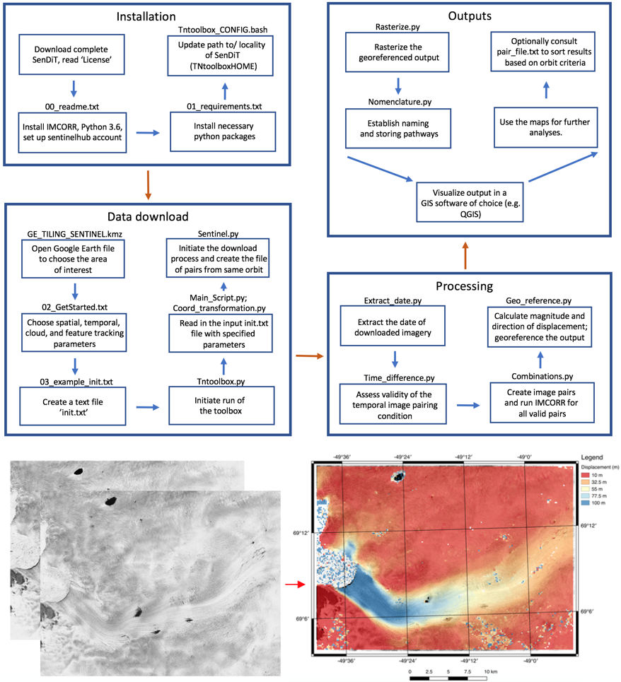
SenDiT provides displacement fields for all image pairs adhering with specified temporal feature tracking parameters. The pairs with the same-orbit imagery were later identified and information was supplied to a user in a separate text file. Within the toolbox, there is no distinction between the imagery from the 2A and 2B missions. The primary intention of the toolbox is for it to be used over moving targets, specifically glaciers, but also other mass wasting movements such as major landslides. To test the toolbox functionality over moving targets, outlet glaciers Engabreen, Nigardsbreen, Tunsbergdalsbreen, Stigaholtbreen and Rembedalskåka (mainland Norway) alongside with Skeiðarárjökull (Iceland), Jakobshavn Isbræ (Greenland), and Tasman Glacier (New Zealand) were selected for analysis.

3.1. Performance over Stable Ground

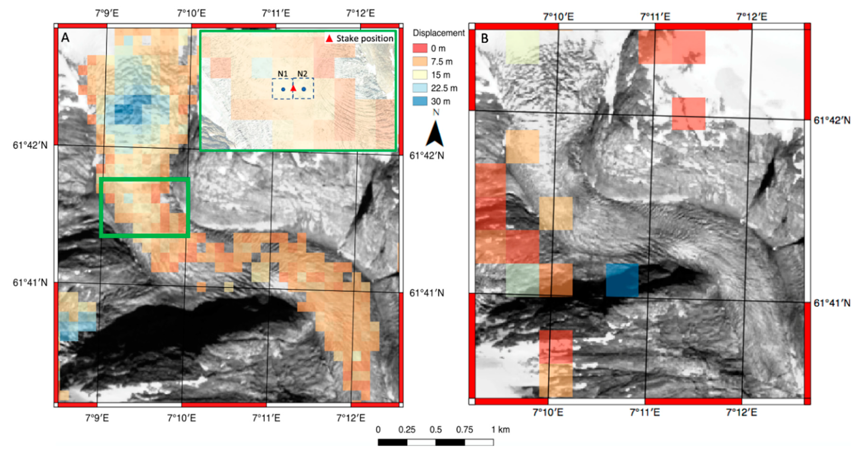
The arid areas in Libya and Australia were chosen as they offer superior quality due to good visual contrast, richness of terrain features, no expected terrain changes, no snow, low probability of cloud cover and remoteness from inhabited areas, or worked farmland. The coverage of potentially moving targets such as rivers, and coverage of homogeneous surfaces such as pure sand was minimized and eliminated by visual inspection where possible. We attempted to maximize spatial coverage of both stable areas, while avoiding homogeneous sand, farmed land, rivers, and water bodies. The arid areas in Libya and Australia were thought to be superior to areas of stable terrain in the proximity to glaciers due to absence of snow cover, cloud cover, and absence of large bodies of water such as proglacial lakes hindering the performance of feature tracking and maximizing the size of the sample for the analysis. The first stable area (Figure 4A) was located in the Northern Territory state of Australia and was dominated by several prominent ridges, surrounded by flat and rugged terrain. The second stable area in Libya (Figure 4B), was dominated by a series of valleys cutting through the rugged terrain, with a minimal extent of the homogeneous sand cover.

Only imagery with less than 1% cloud cover was used for analysis. This imagery was further manually inspected and filtered to eliminate imagery with even minimal presence of clouds. Imagery across both stable areas was paired using the same feature tracking parameters to make the two areas statistically comparable. The effect of seasonality on image pairing is known and studies have underlined importance of keeping the temporal separation to minimum in order to avoid changes in illumination conditions, shadowing, snow cover, but also vegetation [1,24]. Hence, the temporal difference was kept to a minimum; 10 days for single mission combination and 5 days for a 2A–2B mission combination to keep the influence of varying lighting conditions to a minimum. To analyze the role of mission pairing, we used results of 20 pairs over the stable ground in Libya and 28 pairs over the stable ground in Australia. Out of 48 pairs, 23 pairs were paired using Sentinel 2A–2B combination and 25 pairs were paired using either Sentinel 2A–2A or Sentinel 2B–2B combination. Twenty-one out of 25 pairs using a combination of imagery from the same mission were found to have mean displacement, within a 95% confidence interval (2σ) of less than 4 m, which corresponds to less than 0.4 pixels of the 10 m band. On the other hand, only three out of 23 pairs using Sentinel 2A–2B imagery combination led to a mean of less than 4 m within a 95% confidence interval (2σ). From the analysis using a limited number of pairs, it became clear that displacement magnitude of the pairs with a combination of Sentinel-2A and Sentinel-2B imagery was higher than when using single mission acquisitions for the pair.

Many glaciated areas are located in the steep mountainous terrain where shadowing can affect feature tracking. Shadowing can (a) be misrepresented as a moving feature and introduce outliers, as well as (b) result in a complete loss of trackable features due to a change of the pixel intensity values. Shadowing on glacier surface can be due to crevassing, large debris, or the surrounding mountainous topography and it is advantageous to understand how displacement estimation can change in response to changes in illumination conditions. To analyze the effect of the temporal differences on displacement estimation, we used pairs with a wide range of temporal separation (20–140 days), which closely resembled the minimum and maximum separation within a typical melt season, with useful imagery. Using the linear regression for the relationship between the temporal difference and displacement, we found a degree of dependence (R² = 0.44) for 25 pairs over the stable area in Libya. Increase in the displacement over stable ground with increasing time separation of the image pair was likely due to the changing lighting conditions manifesting by introduced shadowing that becomes more extensive with larger temporal gaps. This suggests that the number of outliers can increase with an increase in the temporal separation of the image pair.

The health of the optical sensor is critical for the usefulness of acquired imagery. Most satellite imagery is obtained using push-broom or whiskbroom systems, which can be subjected to jitter [25], or sensor misalignment [26]. Problems with sensor geometry have been identified in the Sentinel-2A satellite [27] and are found to be present in other systems such as ASTER [25], but also Quickbird and SPOT satellites [26]. Satellite imagery can also be subjected to data voids due to failure of the scan line corrector (SLC), as has been the case of the Landsat 7 ETM+ mission for acquisitions since 2003. This resulted in ~22% of pixels not being scanned [28]. While studies have tried to correct for the missing or erroneous data [25,28], other studies have taken a non-inclusive data approach, eliminating the faulty images [29]. Satellite platform vibration induced by the onboard dynamic components and exterior perturbation deteriorates platform stability and causes attitude jitter, resulting in image distortion and geometric accuracy degradation [30]. The multi spectral instrument of the Sentinel 2A-2B constellation operates with a push-broom concept, where the push-broom sensor works by collecting rows of image data across the orbital swath and utilizes the forward motion of the spacecraft along the path of the orbit [31]. With 12 push-broom modules covering each swath, the misregistration of the push-broom data can lead to bias and characteristic stripe pattern of the images. Each swath is approximately 290 km wide [31] and this pattern can therefore be visible in orbit direction mimicking the orbit track each ~24 km.

Our analysis showed the presence of images with a detrimental effect on the displacement measurement results via jitter manifesting in bands of differential displacement within a single push-broom module as well as across more push-broom modules within a single scene (Figure 4D). The bands of differential displacement were found to reach magnitudes of up to 16 m and wavelengths of ~2.5–6 km. Considering the orbital speed of ~7 km/second of the Sentinel 2A satellite [31], the jitter undulations could have been occurring with a period of ~0.33–0.87 s per undulation. Also, the analysis found image pairs (Figure 4C) to be subjected to striping at ~24 km width in the orbit direction, corresponding to the width of each of the 12 adjacent push-broom sensor modules. Equally, [27] reported some image pairs to be subjected to striping at ~20 km width in the orbit direction that was interpreted to be due to misalignments in the overlap areas of 12 adjacent push-broom modules covering the Sentinel-2 swath width of 290 km. Given the maximum cloud cover threshold of 30%, only two images with significant jitter effect were found for the stable area in Libya from 06.09.2015 and 04.01.2016, respectively. No image pairs with push-broom and in-push-broom error patterns attributed to jitter were found after June 2016 in the stable area in Libya, for either the Sentinel-2A or the Sentinel-2B mission, confirming that the jitter error has been rectified by ESA after that date [31].

3.2. Main Sources of Error

When considering sources of movement in a displacement map, there are three main components of it: true movement over a number of days of the pair; co-registration accuracy error; and orthorectification error. Displacement maps can also be affected by jitter as well as failures of parts of the system as explained in Section 3.1. Correction of the Sentinel-2A jitter effect after June 2016 improves the co-registration accuracy that could have reached 18 m before that date [32]. However, it is worth noting that this error did not affect all scenes up to June 2016. According to Castriotta and Knowelden [23], the relative co-registration accuracy of any two images should at the moment be less or equal to 1.12-pixel size (11.2 m for the 10 m bands), with a 95% (2σ) confidence interval. In our analysis of 48 pairs over the stable areas in Libya and Australia, the largest co-registration accuracy error was found to be 10.9 m (2σ), corresponding to ca. 1.09 pixels. Co-registration error will often manifest itself as a homogeneous translation with almost uniform displacement magnitude and displacement vector direction. When using imagery from the same orbit, the co-registration error should be the main source of error [27].

Sentinel-2A and Sentinel-2B scenes are provided as the orthorectified L1C (Level-1 Corrected) products. Two types of errors contribute to vertical offsets between the terrain and its approximation by a Digital Elevation Model (DEM): a) measurement or production errors where DEM elevation does not agree with terrain elevation at the time of acquisition of the elevation data; and b) changes in terrain elevation over time between elevation measurement and satellite scene acquisition [27]. To quantify glacier displacement over time, the latter error is the most prominent one, often encountered as the glaciers can lose tens of meters of elevation between the DEM acquisition date and the date a satellite scene is ingested and orthorectified. Equally, the first error type can be also prominent, especially in glaciated regions with steep mountainous terrain where elevation of the slopes immediately bordering the glaciers can affect the elevation detected, depending on the ground resolution and terrain ruggedness. When co-registering the images from the same relative orbit, the DEM effects and most of the orthorectification error will be eliminated [27].

Co-registration accuracy of the images from two different, usually immediately adjacent orbits will be influenced by the orthorectification as well as co-registration errors. The orthorectification error will reach its maximum in steep mountainous areas, where the terrain itself induces errors in the DEM, and over the ablation zones of alpine glaciers, especially glacier tongues where extensive melting may have occurred in the time gap between the DEM acquisition and satellite image orthorectification. Sentinel-2A and Sentinel-2B constellation imagery is orthorectified using the Planet DEM 90, and other non-specified DEMs for the areas outside the Shuttle Radar Topography Mission (SRTM) coverage (North of 60° latitude) [27]. The Planet DEM 90 is of 90 m resolution, and it is mainly derived from SRTM DEM, which was acquired in February 2000 [33]. There is very limited documentation on the Planet DEM 90 and other DEMs used for the orthorectification of Sentinel-2 imagery. The uncertainty of the Planet DEM 90 is 16 m (2σ) [32]. Unavailability of the Planet DEM 90 makes it hard to understand exact magnitude of DEM errors as well as the mechanisms used to fill in the voids left in the SRTM data.

To test the orthorectification error in practice, we used a pair with a minimal temporal baseline difference of two days over Skeiðarárjökull glacier (64°07’N 17°15’W) in Iceland (Figure 5A). The measured displacement reached magnitudes of over 35 m around the glacier lateral margins and terminus. The mean of apparent displacement of the stable area West of the glacier was ~6.7 m. The prominent vector direction of movement in the stable area was ~180–215°, so the co-registration error shift was in the south direction (Figure 5B). Considering the orthorectification error component alone, the terminal portion of the glacier tongue where such error is expected to be at its maximum can be looked at in detail. In the case of this pair, the apparent displacement magnitude appeared to gradually increase within 1–4 km from the terminal and East lateral glacier margins from ~16–18 m to ~35 m or more (Figure 5C). The temporal gap between the SRTM DEM acquisition in February 2000 and imagery acquisition in August 2017 was ~17.5 years. In this time, the glacier had retreated up to 3 km from its position in summer 1999 to where it was in August 2017 (Figure 5C). A large portion of the displacement seen in Figure 5A,C can be attributed to the orthorectification error as the areas with the highest error magnitude are within the space where the glacier has retreated.. The gradual nature of the error increase towards the terminus suggests continuous thinning with a maximum at the termini. While the DEM used for orthorectification of the Icelandic imagery may not have necessarily come from 2000, the nature of the error and its largest magnitude in areas where the retreat occurred suggest that orthorectification was performed with a regional DEM from a similar point in time. Considering the movement over the two days in the glacier terminus as negligible, the orthorectification error alone is the dominant source of error. Though, in parts of the glacier with less elevation change over the period between the DEM acquisition and date of imagery acquisition the orthorectification error component will be reduced. However, a magnitude of error is unacceptable in most studies and therefore results from using pairs with imagery from different orbits must be treated with caution. With the trend of glacier thinning and retreat over the past ~19 years, the displacement maps of the glacier termini using the imagery sourced from different orbits will present a major source of error. If Sentinel-2 imagery will continue to be orthorectified by Planet DEM 90, which is mostly based on the SRTM DEM acquired in 2000, but also on other regional DEMs [27], the magnitude of orthorectification error component will keep increasing if glacier thinning continues. However, the elevation changes of each glacier will vary. In the case of Skeiðarárjökull, the orthorectification error component is reduced further upstream. To further analyze the orthorectification error component, pairs from 22.08.2017–25.08.2017 and 25.08.2017–27.08.2017 were used to record the maxima of the displacement at glacier termini of Nigardsbreen and Stigaholtbreen in mainland Norway, which retreated 367 m and 130 m respectively in period 2007–2017 [34]. The maxima reached 17.6 m for Nigardsbreen and 18.4 m for Stigaholtsbreen. Having analyzed the displacement over the 22.08.2017–16.09.2017 pair, it was clear that such a large displacement at the glacier termini was due to imagery coming from different relative orbit introducing orthorectification error. The orthorectification errors over Skeiðarárjökull, Nigardsbreen and Stigaholtsbreen were comparable to errors reported by Kääb et al. [27] for Aletschgletscher, Findelengletscher and Gornergletscher in the Swiss Alps, where in all cases, magnitude of displacement reaches tens of meters.

3.3. Application over Glaciers

A range of glaciers was selected to include glaciers with diverse dynamics, dimensions and ice cover characteristics. Using a fast-moving glacier was required to test the maximum magnitude of observable displacement using the toolbox. Jakobshavn Isbræ (69°06’N 49°20’W) was the fastest outlet glacier of the Greenland ice sheet, and can reach velocities of 14,000–16,000 m/year [35]. The velocities were at the highest near the terminus at the grounding line, where Lemos et al. [16] reported an average velocity of ~13,000 m/year for the period between 2014 and 2017, translating to a maximum of approximately 35 m/day. Application of the toolbox over Jakobshavn Isbræ illustrated the practicality of having prior knowledge of maximum expected displacement for the analysis. With a range of different feature tracking parameters, displacement at the short 5-day temporal gap and longest possible 25-day temporal gap was calculated. The temporal difference of 25 days was found to be the maximum baseline for Jakobshavn Isbræ. While the displacement field was, in the case of a 5-day temporal difference, only affected by the presence of supraglacial lakes and changes in the appearance of calved ice behind the grounding line (Figure 6A), in the latter case, it is believed to have been affected by one or a combination of: a) a change in the direction of the ice flow causing decorrelation and non-translational change to feature appearance; b) a displacement too large, which falls outside the search window region (Figure 6B). Therefore, as the specific region has a good coverage from four different orbits, it is more likely to obtain smooth displacement fields using pairs with the shortest time gap possible of 5 and 10 days respectively. The certain true observable maximum of the movement of any glacier, detectable with the toolbox is 620 m but this can reach ca. 880 m in cases of NE, SE, SW, and NW movement.

Analysis over the Tasman glacier was performed to study the possibility of obtaining the displacement field over a debris covered glacier. The Tasman glacier (43°36’S 170°13’E) is New Zealand’s longest and largest glacier fed by numerous tributaries, and extensively covered by debris in its lower portion [13]. The displacement field over the debris covered parts has a smooth appearance (Figure 6C). The quality of the result over debris covered glaciers is in general likely to be influenced by the distribution and appearance of the debris. A perfectly smooth, homogeneous debris cover will likely yield no useful results. On the other hand, variety in distribution of the debris, certain roughness of the terrain as well as the presence of supraglacial lakes, such as in the case of the Tasman glacier, all help to form the features that are both trackable and resistant to change. Figure 6C also illustrates the differences in the level of noise in an image pair. While there was a generally homogeneous apparent displacement over the stable area in the valley adjacent east of the glacier, the magnitude of outliers in the snow-covered parts of the glacier can reach over 60 m.

To illustrate the system performance over the narrow, alpine glaciers, Nigardsbreen, Engabreen and Rembedalskåka glaciers from mainland Norway were selected. All three glaciers have long mass balance measurement time series [34]. The glaciers also belong to a group that have stake velocity measurement data in Norway, which can serve for ground truthing. Rembedalskåka (60°32’N 7°21’E) is a southwestern outlet glacier flowing from the Hardangerjøkulen ice cap, Nigardsbreen (61°42’N 7°09’E) is a southern outlet of the Jostedalsbreen ice cap and Engabreen (66°40’N 13°48’E) is a northwestern outlet of West Svartisen ice cap [34].

Stake point measurement data was available only for a handful of mass balance stakes on each of the trio of glaciers. The stakes were usually located in the interior of the glaciers, not in the termini or outlets, where crevassing is predominant. While this crevassing offers potentially good targets for feature tracking, heavy crevassing, relatively fast flow of the outlets and large mass turnover do not offer good conditions for long-term stake surveying. To compare the results of feature tracking obtained by SenDiT with the in situ measurements, three stakes were selected, which maximize a spatial overlap with feature tracking results, as well as a temporal overlap over the surveyed periods (

Table 1. Comparison of velocities from Sentinel-2 feature tracking using SenDiT and stake in-situ measurements.

Glacier	Point	Period (stake)	Velocity (m/day)	Flow Direction (°)	Distance to FT res. (m)	Period (Sentinel)	Velocity (m/day)	Flow Direction (°)
Nigardsbreen	N1	23.08.2017–18.10.2017	0.567+/−0.005	162	44.07	27.08.2017–16.09.2017	0.624+/−0.175	172
	N2				38.60		0.580+/−0.175	187
Rembedalskåka	R1	15.09.2016–24.05.2018	0.141+/−0.0005	241	104.01	22.08.2017–28.07.2018	0.130+/−0.009	236
	R2				116.59		0.148+/−0.009	238
Engabreen	E1	18.10.2016–25.10.2018	0,122+/−0.0004	358	266.77	22.08.2016–26.09.2017	0.155+/−0.016	341
	E2				306.54		0.149+/−0.016	358

).

Displacement at points N1 and N2 on Nigardsbreen was measured using a pair, which has a complete temporal overlap with the stake measurement temporal window (Figure 7A). The resulting feature tracking velocity was found to be within the error limit of the stake measurement. In the case of Nigardsbreen, the displacement field was relatively smooth, with spatially limited sections with no data (Figure 7A). The magnitude of displacement in raster cells surrounding the position of the stake (Figure 7A) was also relatively uniform. Out of a trio of glacier stakes, the stake measurement on Nigardsbreen was closest to the measured displacement (ca. 39 and 44 m away), which likely factors in the overlap of velocity derived by stake measurements and SenDiT. For Rembedalskåka, there was only a partial temporal overlap of approximately 9 months, accounting for ca. half of the total surveying time. With a limited temporal and spatial overlap (stakes positioned ca. 104 and 117 m away) the resulting feature tracking velocity as well as flow direction were found to be very close to data indicated by stake measurement. At the point R2, the result of the feature tracking was within the limit suggested by the stake measurement. On the other hand, the result of feature tracking was just outside the velocity spread suggested by stake measurement at the point R1. On Engabreen, there was a partial overlap of ca. 11 months between the two time periods, which could together with a longer distance (up to ca. 307 m) between the stake and feature tracking measurements account for a fact that stake measurement did not fall within the displacement range of points E1 and E2 indicated by feature tracking results. However, both the flow direction and displacement magnitude differences of ca. 17° and 0.03 m/day at the point E1 were relatively minor and indicated a good performance of SenDiT. Moreover, at the point E2, flow direction of the stake measurement conformed with the result of feature tracking using SenDiT.

To illustrate the system performance compared to other services, we conducted analyses using Nigardsbreen and Jakobshaven Isbræ. First, an analysis was conducted over the outlet of Nigardsbreen using the results of SenDiT and GoLIVE service. The GoLIVE service is currently the only service providing continuously updated velocity data for the glaciated areas outside the Ice Sheets. For the ablation season of 2017, we were able to identify only one pair from the GoLIVE service with a temporal separation of 32 days, using images from 22.08.2017 and 23.09.2017, respectively. Given the full temporal overlap of the pair used by SenDiT (Figure 7A) with the pair from the GoLIVE service (Figure 7B), we compared their spatial coverage over Nigardsbreen outlet south of 61°43’N. While SenDiT results spatially covered ca. 2.15 km², the resulting velocity field of the GoLIVE product covered ca. 0.36 km². Unlike the SenDiT result (Figure 7A), the GoLIVE’s result (Figure 7B) was reduced to four data points, that could be attributed to noise, compared to ca. 240 data points using SenDiT.

To address the comparison of GoLIVE, MEaSURE, and SenDiT performance over a single site, further analysis was conducted over Jakobshaven Isbræ. When acquiring the velocity maps, close attention was paid to maximization of the temporal overlap among the pairs to provide the best possible results for a comparison. The smoothest velocity fields were provided by the pair J3 derived by SenDiT (Figure 8A) and J6 from the MEaSURE service (Figure 8D). Pairs J4 (Figure 8B) and J5 (Figure 8C) also provided smooth velocity fields, though decorrelated sections were present, corresponding to less than ca. 5% of the entire study area of Jakobshaven Isbræ. Velocity differences between the SenDiT pair J3 (18.07.2017–28.07.2017) and (1) GoLIVE pair J5 (18.07.2017–03.08.2017) and (2) MEaSURE pair J6 (01.07.2017–31.07.2017) were less than 0.5 m/day for most of the studied area. Larger differences occurred in the areas of a fast ice flow and reached up to ca. 2.5 m/day. The velocity difference analysis between the SenDiT derived pair J4 (18.07.2017–03.08.2017) using imagery from different relative orbits and GoLIVE pair J5 (18.07.2017–03.08.2017) with the same temporal separation and the complete temporal overlap, showed large differences of 2–3.5 m/day for most of the area, reaching up to ca. 5 m/day (Figure 8G). Considering the fast nature of the movement of Jakobshaven Isbræ and only a partial temporal overlap, SenDiT produced comparable results to both GoLIVE and MEaSURE services, when using a pair, composed of imagery from the same orbit (Figure 8E,F). Large differences of up to 5 m/day (ca. 80 m displacement) depicted by the Figure 8G can be attributed to the orthorectification error.

4. Discussion

There are several available tools for feature tracking of imagery and derivation of displacement maps. However, there is currently no available tool that would allow for the same degree of flexibility as SenDiT. Compared to the CPOM service, the toolbox allows for acquisition of glacier displacement over any area of the world within a coverage of the Sentinel-2 missions. While GoLIVE system provides world-wide glacier velocity maps, it only includes glaciers larger than 5 km², which excludes many of the alpine glaciers. Unlike GoLIVE, SenDiT also offers flexibility in choosing the temporal separation between the two images, as well as feature tracking parameters, both of which must have the ability to vary as they are highly-individual for each glacier or glaciated region. The GoLIVE system, which is currently the only service that regularly updates velocity maps outside the Ice Sheets, processes imagery acquired by Landsat 8 every 16 days, which makes SenDiT ca. three times more likely to work with a useful image. On the other hand, while SenDiT uses imagery of higher 10 m resolution, GoLIVE system’s output includes also displacement maps from seasons 2013 and 2014, which is not possible for SenDiT using earliest Sentinel-2A imagery from 2015. The spatially superior performance of SenDiT to GoLIVE using Nigardsbreen as the test site showed that flexibility in adjusting feature tracking parameters is key for acquiring valuable displacement information over alpine glaciers. The SenDiT derived velocity field over Jakobshaven Isbræ showed differences of less than 0.5 m/day for most of the studied area, when compared to the MEaSURE and GoLIVE velocity fields. This indicates that SenDiT also performs well over the fast-flowing ice on the Ice Sheet and provides comparable results to currently available MEaSURE and GoLIVE data for Jakobshaven Isbræ.

SenDiT is a novel open-source toolbox with no licensing burden, which automatizes the entire process of acquisition of the displacement maps, except for the filtering of the results, which is left to the user. The degree of flexibility is higher than offered by other services such as CPOM, GoLIVE, and MEaSURE. Automatisation of the process is novel and is not offered by other feature tracking tools such as ImGRAFT or COSI-Corr. SenDiT can yield an unprecedented number of displacement maps in a short time, while giving the user full control over the result, but also provides a balance by requiring only the most essential data input. Creating a tool, which is easy to install and operate was a priority, so that the acquiring of the terrain displacement data from optical imagery can be presented to both skilled, and less experienced users. By making a toolbox attractive to a wider audience, SenDiT has the potential to be used by a larger number of users than previously developed feature tracking software. With the increased number of the users, the toolbox can kindle more widespread research activity.

The toolbox is demonstrated to work successfully over a range of glaciers. It was applied to the Engabreen, Nigardsbreen, Tunsbergdalsbreen, Stigaholtbreen and Rembedalskåka glaciers in Norway, as well as Skeiðarárjökull in Iceland, Jakobshavn Isbræ in Greenland and the Tasman Glacier in New Zealand, with results over narrow, debris covered and fast-moving glaciers (

Table 2. Summary of maximum velocities from Sentinel-2 feature tracking using SenDiT on example glaciers.

Glacier	Country	Period (Sentinel)	Max. Velocity (m/day)	Flow Direction	Debris Cover
Nigardsbreen	Norway	27.08.2017–16.09.2017	1.62+/−0.175	S/SE	No
Rembedalskåka	Norway	22.08.2017–28.07.2018	0.15+/−0.009	W	No
Engabreen	Norway	22.08.2016–26.09.2017	0.16+/−0.016	N/NW	No
Jakobshaven I. 1	Greenland	29.07.2017–03.08.2017	32.4	W/NW	No
Jakobshaven I. 2	Greenland	21.07.2017–15.08.2017	29.8	W/NW	No
Jakobshaven I. 3	Greenland	18.07.2017–28.07.2017	32.5	W/NW	No
Jakobshaven I. 4	Greenland	18.07.2017–03.08.2017	33.1	W/NW	No
Tasman Glacier	New Zealand	29.09.2017–11.02.2018	0.51+/−0.08	S/SE	Yes

Error for Jakobshaven Isbræ pairs is omitted due to small sample of a stable area.

). Using selected stake measurement data over a trio of Norwegian glaciers (Nigardsbreen, Engabreen, Rembedalskåka), the stake velocity was found to be within the error margin of the feature tracking measurements provided by SenDiT for Nigardsbreen and Rembedalskåka. Partial disagreement between the measured stake velocity and results of SenDiT for Engabreen are likely due to a reduced spatial and temporal overlap between the two measurements. Overall, this indicates a good performance of the toolbox despite the differences in the case of Engabreen that should be thought of as relatively minor. Maximum velocities for a range of glaciers that we used SenDiT for were approximately 33 m/day for Jakobshavn Isbræ, 0.5 m/day for Tasman Glacier, and 1.6 m/day for Nigardsbreen (Table 2).

The current version of the toolbox exclusively supports the Sentinel-2 imagery, with the highest resolution being 10 m. With the onset of new Landsat and Sentinel missions in the coming years, this may change as the wealth of data increases. The current version of the toolbox does not include result filtering, leaving that additional step to the user. Filtering of the output is subjective to each application of the tool.

While there are limitations that predetermine the accuracy of the toolbox, the user is given full control over the choice of parameters. The quality of the displacement results from SenDiT will in the first instance depend on the choice of pairs coming from the same versus different relative orbit. If a pair comprised of images from two different orbits is used, it will be more prone to orthorectification error, which was shown to be prominent over Skeiðarárjökull, where it amounted to over 35 m. The results over Nigardsbreen and Stigaholtbreen termini reaching magnitudes of 17.6 and 18.4 m further confirmed that the error magnitude can be in tens of meters. These results agree with results of Kääb et al. [27] that reported orthorectification error magnitudes of several tens of meters over glaciers in the Swiss Alps. Additionally, the velocity difference of up to ca. 5 m/day corresponding to ca. 80 m of displacement observed comparing the SenDiT derived pair J4 and GoLIVE pair J5 suggests that the magnitude of the orthorectification error can be substantially larger over the sections of the Ice Sheet. Co-registration error, using imagery from the same orbit was found to be larger than 4 m (2σ) for 87% of image pairs using the Sentinel 2A–2B combination and 16% with either the Sentinel 2A-2A or Sentinel 2B–2B combination. While in the current version of the toolbox the user has no control over the ‘in-pair’ mission combination criteria, our results suggest that pairs coming from the same mission may need to be prioritized when acquiring displacement fields, in particular over slow moving glaciers. Temporal separation of a matched pair can also affect quality of matching. Using 25 pairs over the stable area in Libya with temporal separation of 20–140 days, we observed an increasing trend of mean displacement with increasing temporal separation, likely caused by shadowing induced outliers. Images from before June 2016 may be subjected to jitter error resulting in pairs of limited value [23]. Using 41 pairs over the stable area in Libya, we identified only two images subjected to jitter error, of which the latest one came from 04.01.2016. While some image pairs from before June 2016 can be affected [32], there is still plenty of unaffected imagery from the summer and winter season 2015.

5. Conclusions

This work presents the application and development of a semi-automatic toolbox for retrieving displacement maps, which automatically downloads, and processes imagery given the set of input requirements specified by individual user. Currently, there is no available tool that would allow for the same degree of flexibility as SenDiT. The toolbox uses the current highest resolution freely-available imagery from the Sentinel 2A–2B constellation and it is free to use and can be applied to track the movement of glaciers as well as other mass movements, with sufficient magnitude of displacement. The number of key input parameters has been kept to minimum. The key parameters that are used for the toolbox to run are: extent of the surveyed area, time of acquisitions, time window for image pairing, and feature tracking parameters. The main output are rasterized georeferenced maps of displacement and direction of the movement. The system currently processes the Sentinel-2A and Sentinel-2B imagery, with the earliest imagery acquired after 23.06.2015. The amount of available acquisitions has doubled after the launch of Sentinel-2B mission on 07.03.2017. The user is provided with all displacement maps and vector direction maps adhering to the specified temporal criteria. The text file supplied with the output provides a list of pairs from the same relative orbit, which should be the first ones to be consulted. The SenDiT is demonstrated to work successfully over a range of glaciers. This work presents its application over Engabreen, Nigardsbreen, Tunsbergdalsbreen, Stigaholtbreen and Rembedalskåka glaciers in Norway as well as, Skeiðarárjökull in Iceland, Jakobshavn Isbræ in Greenland and Tasman Glacier in New Zealand, with results over narrow, clean and debris covered as well as fast glaciers. It is also tested on areas of stable terrain in Libya and Australia, where sources of error involved in the feature tracking using Sentinel-2 imagery are thoroughly described and quantified. The toolbox can be used further to provide a regional and global set of ice velocity change over specified timeframes. It can be also modified for analyses of future higher resolution imagery.

References

1. Dehecq, A.; Gourmelen, N.; Trouve, E. Deriving large-scale glacier velocities from a complete satellite archive: Application to the Pamir–Karakoram–Himalaya. Remote Sens. Environ. 2015, 162, 55–66. [Google Scholar] [CrossRef] [Green Version]
2. Li, J.; Roy, D.P. A global analysis of Sentinel-2A, Sentinel-2B and Landsat-8 data revisit intervals and implications for terrestrial monitoring. Remote Sens. 2017, 9, 902. [Google Scholar] [CrossRef]
3. Lucchitta, B.K.; Ferguson, H.M. Antarctica: Measuring glacier velocity from satellite images. Science 1986, 234, 1105–1108. [Google Scholar] [CrossRef] [PubMed]
4. Bindschadler, R.; Scambos, T. Satellite-image-derived velocity field of an Antarctic ice stream. Science 1991, 252, 242–246. [Google Scholar] [CrossRef]
5. Bernstein, R. Image geometry and rectification. In Manual of Remote Sensing; American Society of Photogrammetry: Falls Chyrch, VR, USA, 1983; pp. 881–884. [Google Scholar]
6. Fitch, A.J.; Kadyrov, A.; Christmas, W.J.; Kittler, J. Orientation correlation. In Proceedings of the British Machine Vision Conference, Cardiff, UK, 2–5 September 2002; pp. 133–142. [Google Scholar]
7. Michel, R.; Rignot, E. Flow of Glaciar Moreno, Argentina, from repeatpass shuttle imaging radar images: Comparison of the phase correlation method with radar interferometry. J. Glaciol. 1999, 45, 93–100. [Google Scholar] [CrossRef]
8. Fahnestock, M.; Scambos, T.; Bindschadler, R.A. Semi-automated ice velocity determination from satellite imagery. EOS 1992, 73, 493. [Google Scholar]
9. Leprince, S.; Barbot, S.M.; Ayoub, F.; Avouac, J.P. Automatic and precise orthorectification, coregistration, and sub-pixel correlation of satellite images, application to ground deformation measurements. IEEE Trans. Geosci. Remote Sens. 2007, 46, 1529–1558. [Google Scholar] [CrossRef]
10. Messerli, A.; Grinsted, A. Image georectification and feature tracking toolbox: ImGRAFT. Geosci. Instrum. Methods Data Syst. 2015, 4, 23–34. [Google Scholar] [CrossRef] [Green Version]
11. Heid, T.; Kääb, A. Evaluation of existing image matching methods for deriving glacier surface displacements globally from optical satellite imagery. Remote Sens. Environ. 2012, 118, 339–355. [Google Scholar] [CrossRef]
12. O’Neel, S.; Pfeffer, W.T.; Krimmel, R.; Meier, M. Evolving force balance at Columbia Glacier, Alaska, during its rapid retreat. J. Geophys. Res. 2005, 110, F03012. [Google Scholar] [CrossRef]
13. Redpath, T.A.N.; Sirguey, P.; Fitzsimons, S.J.; Kääb, A. Accuracy assessment for mapping glacier flow velocity and detecting flow dynamics from ASTER satellite imagery: Tasman Glacier, New Zealand. Remote Sens. Environ. 2013, 133, 90–101. [Google Scholar] [CrossRef]
14. Joughin, I.; Smith, B.; Howat, I.; Scambos, T.; Moon, T. Greenland flow variability from ice-sheet-wide velocity mapping. J. Glaciol. 2010, 56, 415–430. [Google Scholar] [CrossRef]
15. Fahnestock, M.; Scambos, T.; Moon, T.; Gardner, A.; Haran, T.; Klinger, M. Rapid large-area mapping of ice flow using Landsat 8. Remote Sens. Environ. 2016, 185, 84–94. [Google Scholar] [CrossRef] [Green Version]
16. Lemos, A.; Shepherd, A.; McMillan, M.; Hogg, A.E.; Hatton, E.; Joughin, I. Ice velocity of Jakobshavn Isbrae, Petermann Glacier, Nioghalvfjerdsfjorden, and Zachariae Isstrom, 2015-2017, from Sentinel 1-a/b SAR imagery. Cryosphere 2018, 12, 2087–2097. [Google Scholar] [CrossRef]
17. Scambos, T.; Fahnestock, M.; Moon, T.; Gardner, A.; Klinger, M. Global Land Ice Velocity Extraction from Landsat 8 (GoLIVE), Version 1; National Snow and Ice Data Center: Boulder, CO, USA, 2016. [Google Scholar] [CrossRef]
18. Drusch, M.; Del Bello, U.; Carlier, S.; Colin, O.; Fernandez, V.; Gascon, F.; Hoersch, B.; Isola, C.; Laberinti, P.; Martimort, P.; et al. Sentinel-2: ESA's optical high-resolution mission for GMES operational services. Remote Sens. Environ. 2012, 120, 25–36. [Google Scholar] [CrossRef]
19. Zhang, H.K.; Roy, D.P.; Yan, L.; Li, Z.; Huang, H.; Vermote, E.; Skakun, S.; Roger, J. Characterization of Sentinel-2A and Landsat-8 top of atmosphere, surface, and nadir BRDF adjusted reflectance and NDVI differences. Remote Sens. Environ. 2018, 215, 482–494. [Google Scholar] [CrossRef]
20. Irons, J.R.; Dwyer, J.L.; Barsi, J.A. The Next Landsat Satellite: The Landsat Data Continuity Mission. Remote Sens. Environ. 2012, 122, 11–21. [Google Scholar] [CrossRef]
21. Loveland, T.R.; Irons, J.R. Landsat 8: The plans, the reality, and the legacy. Remote Sens. Environ. 2016, 185, 1–6. [Google Scholar] [CrossRef]
22. Paul, F.; Winsvold, S.H.; Kääb, A.; Nagler, T. Glacier remote sensing using Sentinel-2. Part II: Mapping glacier extents and surface facies, and comparison to Landsat-8. Remote Sens. 2016, 8, 575. [Google Scholar] [CrossRef]
23. Castriotta, A.G.; Knowelden, R. Sentinel Data Access 2017 annual report. Unpublished.
24. Moon, T.; Joughin, I.; Smith, B. Seasonal to multiyear variability of glacier surface velocity, terminus position, and sea ice/ice melange in northwest Greenland. J. Geophys. Res. Earth Surf. 2015, 120, 818–833. [Google Scholar] [CrossRef]
25. Iwasaki, A. Detection and Estimation Satellite Attitude Jitter Using Remote Sensing Imagery. In Advances in Spacecraft Technologies; Hall, J., Ed.; InTech: Rijeka, Croatia, 2011; Volume 13, pp. 257–272. [Google Scholar]
26. Ayoub, F.; Leprince, S.; Binety, R.; Lewis, K.W.; Aharonson, O.; Avouac, J.P. Influence of camera distortions on satellite image registration and change detection applications. In Proceedings of the 2008 IEEE International Geoscience and Remote Sensing Symposium, Boston, MA, USA, 6–11 July 2008. [Google Scholar]
27. Kääb, A.; Winsvold, S.; Altena, B.; Nuth, C.; Nagler, T.; Wuite, J. Glacier Remote Sensing Using Sentinel-2. Part I: Radiometric and Geometric Performance, and Application to Ice Velocity. Remote Sens. 2016, 8, 598. [Google Scholar] [CrossRef]
28. Zeng, C.; Shen, H.; Zhang, L. Recovering missing pixels for Landsat ETM+ SLC-off imagery using multi-temporal regression analysis and regularization method. Remote Sens. Environ. 2013, 131, 182–194. [Google Scholar] [CrossRef]
29. Winsvold, S.H.; Kääb, A.; Nuth, C. Regional Glacier Mapping Using Optical Satellite Data Time Series. IEEE J. Sel. Top. Appl. Earth Observ. Remote Sens. 2016, 9, 3698–3711. [Google Scholar] [CrossRef] [Green Version]
30. Liu, S.; Tong, X.; Wang, F.; Sun, W.; Guo, C.; Ye, Z.; Jin, Y.; Xie, H.; Chen, P. Attitude Jitter Detection Based on Remotely Sensed Images and Dense Ground Controls: A Case Study for Chinese ZY-3 Satellite. IEEE J. Sel. Top. Appl. Earth Observ. Remote Sens. 2016, 9, 5760–5766. [Google Scholar] [CrossRef]
31. Castriotta, A.G. Sentinel Data Access 2016 annual report. Unpublished.
32. Stumpf, A.; Michéa, D.; Malet, J.-P. Improved Co-Registration of Sentinel-2 and Landsat-8 Imagery for Earth Surface Motion Measurements. Remote Sens. 2018, 10, 160. [Google Scholar] [CrossRef]
33. Ressl, C.; Pfeifer, N. Evaluation of the elevation model influence on the orthorectification of Sentinel-2 satellite images over Austria. Eur. J. of Remote Sens. 2018, 51, 693–709. [Google Scholar] [CrossRef]
34. Kjøllmoen, B.; Andreassen, L.M.; Elvehøy, H.; Jackson, M. Glaciological investigations in Norway in 2017; Norges vassdrags- og energidirektorat (NVE): Oslo, Norway, 2018; pp. 1–82. [Google Scholar]
35. Joughin, I.; Smith, B.E.; Shean, D.E.; Floricioiu, D. Brief Communication: Further summer speedup of Jakobshavn Isbrae. Cryosphere 2014, 8, 209–214. [Google Scholar] [CrossRef]
Figure 1. Comparison of Landsat 8 (L8) with Sentinel-2 (S2) and ortophoto (OR) of Nigardsbreen tongue and terminus using imagery acquired on 22.08.2017 (S2 and L8) and on 26.08.2017 (OR). (A) L8 band 8 image of 15 m ground resolution over the area of interest; (B) S2 band 8 image of 10 m ground resolution over the area of interest; (C) Close-up of the image A displaying minimal signs of crevassing; (D) Close-up of ortophoto displaying heavy crevassing in the upstream and lateral sections at 0.25 m ground resolution; (E) Close-up of the image B displaying clear crevassing in the upstream and lateral parts.
Remotesensing 11 01151 g001
Figure 2. Schematic diagram of SenDiT processing chain.
Remotesensing 11 01151 g002
Figure 3. (A) Sentinel-2 image of the Jostedalsbreen ice cap from 11.09.2016 with >75% cloud cover; (B) Sentinel-2 image of the Jostedalsbreen ice cap from 23.07.2016 with minimal cloud cover; (C) Displacement map using pair 23.07.2016–11.09.2016 over a close-up image of a section of Tunsbergdalsbreen with less cloud coverage than overall scene of 11.09.2016; (D) Close-up image of a section of Tunsbergdalsbreen with minimal snow cover and no cloud cover conditions.
Remotesensing 11 01151 g003
Figure 4. (A) Stable area in Australia; (B) Stable area in Libya; (C) Map of displacement of pair 04.01.2016–14.01.2016 over the stable area in Libya displaying striping in the orbit direction; (D) Map of displacement of pair 06.09.2016–06.10.2016 over the stable area in Libya displaying bands of differential displacement in the cross orbit direction. Arrows in (C) and (D) indicate position of striping in the along track direction.
Remotesensing 11 01151 g004
Figure 5. (A) Displacement map of pair 20.08.2017–22.08.2017 over Skeiðarárjökull displaying increased magnitude of displacement at the terminus and lateral regions; (B) Flow direction map of pair 20.08.2017–22.08.2017 over Skeiðarárjökull displaying dominant eastward direction of displacement field over the glacier; (C) Close-up displacement map of the terminus of Skeiðarárjökull and position of the snout on 22.08.2017 and 06.08.1999. Pixels with no displacement data are left blank.
Remotesensing 11 01151 g005
Figure 6. (A) Displacement map of pair J1: 29.07.2017–03.08.2017 over Jakobshavn Isbræ displaying smooth displacement signal over entire glacier with maxima of over 155 m at the terminus; (B) Displacement map of pair J2: 21.07.2017–15.08.2017 over Jakobshavn Isbræ displaying decorrelated displacement signal at the terminus and at the sharp change in flow direction; (C) Displacement map of pair 29.09.2017–11.02.2018 over the Tasman Glacier showing smooth displacement signal across the debris covered part of the glacier.
Remotesensing 11 01151 g006
Figure 7. (A) SenDiT derived displacement map of pair 27.08.2017–16.09.2017 over Nigardsbreen outlet glacier with a close-up image of a position of the stake and points N1 and N2 over orthophoto from 26.08.2017 with 0,25 m ground resolution; (B) GoLIVE service displacement map of pair 22.08.2017–23.09.2017 over Nigardsbreen outlet.
Remotesensing 11 01151 g007
Figure 8. Velocity maps of Jakobshaven Isbræ for: (A) pair J3: 18.07.2017–28.07.2018 using SenDiT; (B) pair J4: 18.07.2017–03.08.2017 using SenDiT; (C) pair J5: 18.07.2017–03.08.2017 using GoLIVE; (D) pair J6: 01.07.2017–31.07.2017 using MEaSURE. Velocity difference maps for: (E) pairs J3 and J5; (F) pairs J3 and J6; (G) pairs J4 and J5.
Remotesensing 11 01151 g008