Article

Parcel-Based Crop Classification Using Multi-Temporal TerraSAR-X Dual Polarimetric Data

Faculty of Agriculture, Shizuoka University, Shizuoka 422-8529, Japan
Remote Sens. 2019, 11(10), 1148; https://doi.org/10.3390/rs11101148
Submission received: 17 April 2019 / Revised: 7 May 2019 / Accepted: 11 May 2019 / Published: 14 May 2019
(This article belongs to the Special Issue Radar Remote Sensing for Agriculture)

Abstract

:
Cropland maps are useful for the management of agricultural fields and the estimation of harvest yield. Some local governments have documented field properties, including crop type and location, based on site investigations. This process, which is generally done manually, is labor-intensive, and remote-sensing techniques can be used as alternatives. In this study, eight crop types (beans, beetroot, grass, maize, potatoes, squash, winter wheat, and yams) were identified using gamma naught values and polarimetric parameters calculated from TerraSAR-X (or TanDEM-X) dual-polarimetric (HH/VV) data. Three indices (difference (D-type), simple ratio (SR), and normalized difference (ND)) were calculated using gamma naught values and m-chi decomposition parameters and were evaluated in terms of crop classification. We also evaluated the classification accuracy of four widely used machine-learning algorithms (kernel-based extreme learning machine, support vector machine, multilayer feedforward neural network (FNN), and random forest) and two multiple-kernel methods (multiple kernel extreme learning machine (MKELM) and multiple kernel learning (MKL)). MKL performed best, achieving an overall accuracy of 92.1%, and proved useful for the identification of crops with small sample sizes. The difference (raw or normalized) between double-bounce scattering and odd-bounce scattering helped to improve the identification of squash and yams fields.

1. Introduction

The extent of a cultivated area is an important factor in estimating crop harvest. Crop maps, documenting field properties, including crop type and location, have been generated by some local governments in Japan. However, the documentation of field properties is generally done manually, and the development of easier methods, such as techniques based on satellite remote sensing, is required due to the high cost of existing methods [1].
Optical remote sensing is one of the most attractive options; in particular, Landsat series data have potential in land characterization applications due to their spatial, spectral, and radiometric qualities [2,3,4,5]. Furthermore, the Sentinel-2 satellites have contributed to create greater opportunities for monitoring plant constituents, such as pigments, leaf water contents, and biochemicals [6,7], and the vegetation indices calculated from Sentinel-2 Multispectral Instrument (MSI) data were useful to identify the specific crop types [8,9]. However, optical data are influenced by atmospheric or weather conditions, and the number of available scenes may be restricted. Data from synthetic aperture radar (SAR) systems are an alternative, offering a significant amount of information related to plant phenology, soil moisture, which affects the timing of seeding, transplanting, and harvesting, and vegetation parameters, such as crop height or crop cover rate [10,11,12,13]. SARs are not subject to atmospheric influences or weather conditions, making them suitable in multi-temporal classification approaches [14,15]. Previous studies have shown the potential of C and L-band SAR data to discriminate crop types [16,17], and a significant improvement in classification accuracy has been reported when SAR data and a Landsat8 satellite image time series were integrated [2,18]. Sentinel-1 data have been applied for mapping crop fields with the support of Sentinel-2 data or Landsat-8 data [19,20,21,22]. Besides these, TerraSAR-X and TanDEM-X provide X-band SAR data of high geometric accuracy at a high spatial resolution of 2.5–6 m in 30-km swaths in Stripmap mode [23]. X-band SAR data are now widely available. The backscattering coefficient calculated from SAR data is a function of the geometry and dielectric properties of the target and the amount of biomass in agricultural fields [24]. Therefore, temporal changes can be distinguished using multi-temporal SAR data. The major change in backscatter intensity occurs as a result of ploughing and seeding; smaller changes occur due to variations in the biomass and plant water content, and, for X-band SAR data, in plant structure. Harvesting also causes large backscatter intensity changes [25]. At times, however, no change in backscatter intensity is observed despite geometric changes; this is typically observed for dense vegetation, such as grasslands, and for high-frequency SAR data, such as C-band data [25], and this feature could help us to discriminate some specific crop types, such as grasslands and wheat fields.
Polarimetric decomposition is a promising technique for resolving this problem. In particular, quad-polarimetric observations provide more information than a single polarization and show potential for monitoring and mapping various crops. Several polarimetric decomposition methods have been developed to obtain more information about scattering. However, the doubled pulse repetition frequency leads to a reduced swath width when scanning all polarizations, which limits the opportunities to obtain quad-polarization SAR data. To overcome these problems, compact polarimetric techniques, such as m-chi decomposition [26,27] and dual polarization entropy/alpha decomposition [28], have been proposed. In this study, we examined crop classifications using the polarimetric parameters obtained from the TerraSAR-X dual-polarimetric data (HH and VV polarization).
The radar vegetation index (RVI) is another technique that enhances the characteristic features of vegetation based on SAR data [29,30]. The original RVI is calculated from backscattering coefficients of HH, HV, and VV polarization; this index cannot be extracted from TerraSAR-X dual polarimetric data. However, based on the concept of vegetation indices (VIs) based on optical data that are calculated from simple formulas consisting of a combination of two or more reflectance wavebands, some indices can be calculated using gamma naught or m-chi decomposition parameters. In this study, indices based on differences (D-type index), simple ratios (SRs), and normalized differences (NDs), as well as combinations of these, were considered.
In addition to effective predictors, some supervised learning models may allow for accurate classification; however, different classification algorithms produce different results, even when the same training data are used [31,32]. Support vector machine (SVM) and random forests (RF) are the most effective classification approaches, and some previous studies have shown the strong potential of these techniques for identification of vegetation or soil types using remote-sensing data [33,34]. Extreme learning machines (ELMs) [35] have also exhibited strong performances in terms of classification and regression, and kernel-based ELMs (KELMs) may offer the highest accuracy [32,36,37,38]. In addition to these techniques, recent major advances in Deep Learning Neural Networks are making it possible to solve problems that have resisted the best attempts of the artificial intelligence community [39,40]. Deep learning has a powerful learning capability feature that has been applied to optical remote-sensing data. Other recent techniques based on machine learning are multiple kernel methods, which consist of a convex combination of kernels, with the weight of each kernel optimized during training, and the multiple kernel learning (MKL) [41,42] and multiple kernel extreme learning machines (MKELMs) have been proposed [43]. Although some previous studies provided a comparison of results among various machine-learning algorithms [32], imbalanced data may result in poor classification results, providing worse results than those reported in other studies. In the present study, the abilities of six classification algorithms to identify imbalanced data were evaluated and compared.
The main objectives of this paper are (1) to evaluate the potential of TerraSAR-X data with respect to crop type classification and (2) to identify which algorithms are most suitable for classification in the study area.

2. Materials and Methods
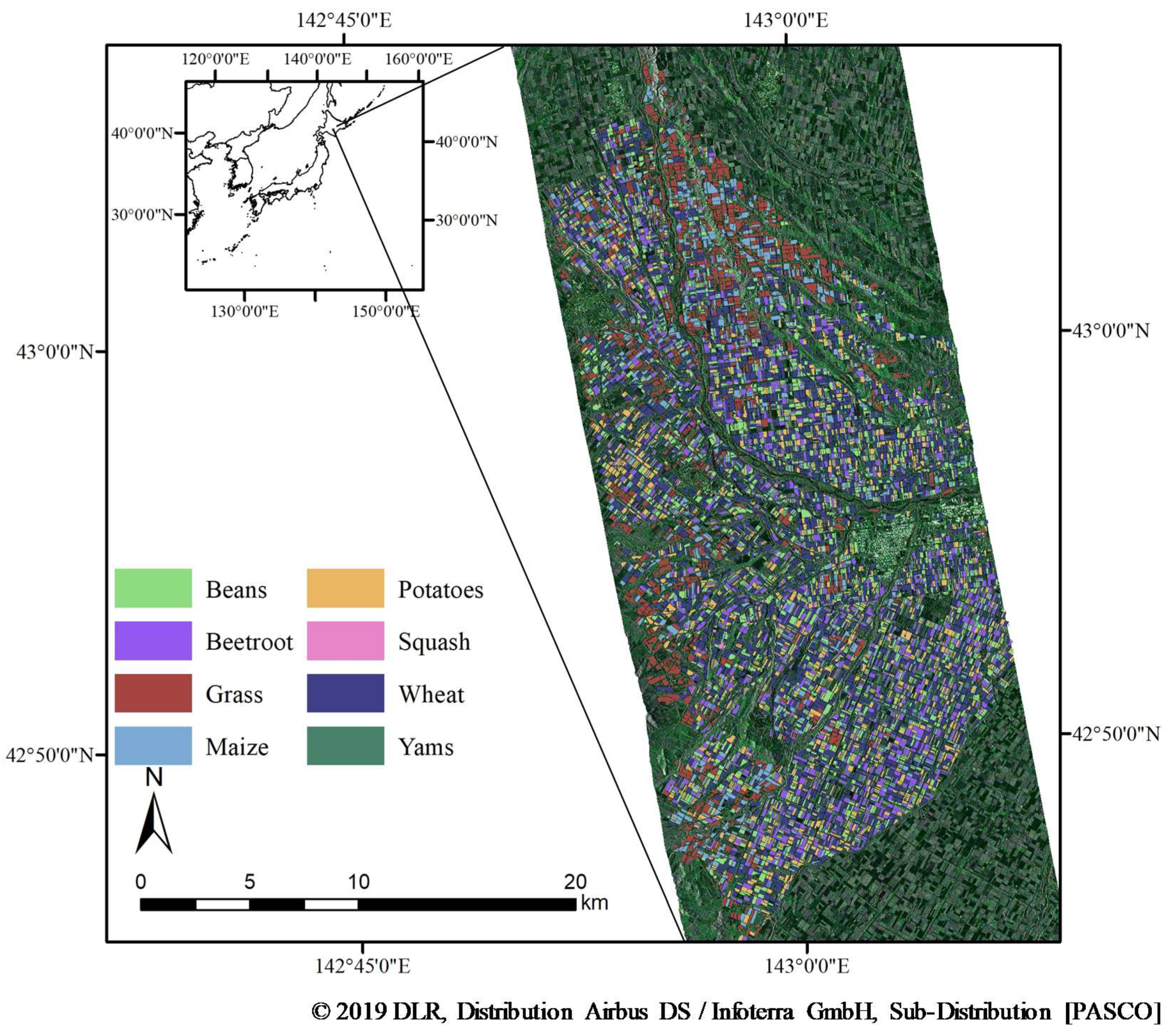
2.1. Study Area

The experimental area of this study is the farming area of the western Tokachi Plain, Hokkaido, Japan (142°42′51″ to 143°08′47″ E, 42°43′20″ to 43°07′24″ N, Figure 1). The study area has a humid continental climate characterized by warm summers and cold winters. The average annual temperature was 6 °C and annual precipitation was 920 mm. The precipitation during the snow-covered period accounts for 32.5%. The cultivated land area per farmhouse is 41.7 ha, which is twice the average area in Hokkaido; however, the agricultural fields are highly fragmented, with many smaller than 1 ha. The dominant crops are beans, beetroot, grassland, maize, potatoes, and winter wheat. Some new crop types have recently been confirmed, although on a much smaller proportion of fields. In particular, squash and yam have become increasingly important crops, with the latter increasing rapidly and having been exported to Taiwan since 1999. The cultivation calendar for this study area is shown in Table 1. For most of the crop types, seeding or transplanting is conducted in late April to mid-May, except for winter wheat (September) and grass (not defined). The harvesting periods are late September to early November for beans, November for beetroot, late August to September for maize and potatoes, mid-September for squash, early to mid-August for winter wheat, and late October for yams. There are two harvesting periods for grasses (timothy and orchard grass), with the first harvest in late June to early July and the second in late August.

2.2. Reference Data

Field location and attribute data, including crop types and area, were obtained based on manual surveys conducted by Tokachi Nosai (Obihiro, Hokkaido), and recorded in a polygon shape file. TerraSAR-X data covered a total of 10,712 fields (1884 bean fields, 1426 beetroot fields, 1445 grasslands, 1029 maize fields, 1564 potato fields, 131 squash fields, 3035 winter wheat fields, and 135 yam fields) that covered the area in 2013. The field size was 0.22–14.85 ha (median 1.88 ha) for beans, 0.25–9.68 ha (median 2.38 ha) for beetroot, 0.20–17.99 ha (median 2.21 ha) for grassland, 0.17–18.72 ha (median 2.56 ha) for maize, 0.26–16.00 ha (median 1.93 ha) for potatoes, 0.21–5.57 ha (median 2.56 ha) for squash, 0.15–17.03 ha (median 2.50 ha) for wheat, and 0.36–6.35 ha (median 1.77 ha) for yams.

2.3. Satellite Data

Ten TerraSAR-X images were acquired in StripMap mode (incidence angle of 42.3°) during ascending passes between 15 May 2013 and 11 August 2013 with an 11-day interval (Table 2). Gamma naught (γº) images (equally spaced, radiometrically calibrated power images) were used, since they are better suited for crop classification than σº images and are less dependent on the incidence angle. In addition to the γº values of HH (γºHH) and VV(γºVV), the polarimetric parameters of the m-chi decomposition (single- or odd-bounce (Odd), double- or even-bounce (Dbl), and randomly oriented (Rnd) scattering) [26,27] and the dual polarization entropy/alpha decomposition (averaged alpha angle and entropy) [28] were obtained using the European Space Agency (ESA)’s PolSARpro SAR Data Processing Educational Tool [44]. The polarimetric parameters were orthorectified using the Alaska Satellite Facility’s MapReady Remote Sensing Toolkit [45], the 10-m mesh digital elevation model (DEM) produced by the Geospatial Information Authority of Japan (GSI), and the Earth Gravitational Model 2008 (EGM2008). The German Aerospace Centre (DLR) commissioning results indicate a geolocation accuracy of 0.3 m in range and 0.53 m in azimuth for TerraSAR-X data [46]; thus, further geometric correction was not conducted. However, all fields were buffered inward by 10 m to avoid selecting training pixels from the edge of a field, which would create a mixed signal and would affect assessment accuracy [15]. To compensate for spatial variability and to avoid problems related to uncertainty in georeferencing, average values of SAR data were calculated for the fields and for each observation using field polygons (shape file format) provided by Tokachi Nosai (http://www.tokachi-nosai.or.jp/). These processes were conducted using QGIS software (version 2.18.27).
Some radar vegetation indices have been proposed for more accurate estimation of vegetation properties, such as height, leaf area index, dry biomass [47], and water content [30]. Difference (D-type), simple ratio (SR), and normalized difference (ND) indices have been widely applied for the development of vegetation indices, including in optical remote sensing. These indices were calculated using gamma naught (γºHH and γºVV) values and m-chi decomposition parameters (Odd, Dbl, and Rnd):
D ( λ 1 , λ 2 ) = P a r a m e t e r   1 P a r a m e t e r   2 ,
SR ( λ 1 , λ 2 ) = P a r a m e t e r   1 / P a r a m e t e r   2 ,
ND ( λ 1 , λ 2 ) = ( P a r a m e t e r   1 P a r a m e t e r   2 ) / ( P a r a m e t e r   1 + P a r a m e t e r   2 ) ,
where Parameter 1 and 2 are one of two gamma naught values or m-chi decomposition parameters, and all 10 combinations were calculated for each index type for all TerraSAR-X data acquired between 16 May 2013 and 22 August 2013.
For dimensionality reduction, which is one of the most popular techniques to remove noisy data, linear discriminant analysis (LDA) was adopted following a previous study [48] using the ‘stepclass’ algorithm, which is included in the ‘klaR’ package [49], before generating classification models. LDA is one of the linear transformation techniques that represents the axes that maximize the separation among multiple classes. At first, the d-dimensional mean vectors are calculated for each class. Next, the eigenvectors and corresponding eigenvalues are calculated from the scatter matrices. After that, the eigenvectors are sorted in descending order and k eigenvectors with the largest eigenvalues are chosen to form a d×k dimensional matrix. Finally, this d×k eigenvector matrix is used to transform the samples onto the new subspace [50].

2.4. Classification Procedure

Based on a previous study [51], a stratified random sampling approach was applied, and the samples were divided into three datasets: a training set (50%), which was used to fit the models; a validation set (25%) used to estimate the prediction error for model selection; and a test set (25%) used for assessing the generalization error in the final selected model (Table 3). This procedure was repeated 10 times (hereinafter, referred to as 1–10 rounds) to produce robust results.
Performance evaluation was carried out for the six algorithms: support vector machine (SVM), random forest (RF), multilayer feedforward neural network (FNN), kernel-based extreme learning machine (KELM), multiple kernel learning (MKL), and multiple kernel extreme learning machine (MKELM). All processes were implemented using R version 3.5.0. [52].
SVM was applied with a Gaussian radial basis function (RBF) kernel, which has two hyperparameters that control the flexibility of the classifier: the regularization parameter C, which is the trade-off parameter between error and margin, and the kernel bandwidth γ, which defines the reach of a single training example. RF is an ensemble classifier that builds multiple decision trees using bootstrapped sampling and a randomly selected subset of the training dataset. In this study, five hyperparameters were optimized: the number of trees (ntree), the number of variables used to split the nodes (mtry), the minimum number of unique cases in a terminal node (nodesize), the maximum depth of tree growth (nodedepth), and the number of random splits (nsplit). Classification approaches based on RF and SVM are equally reliable [53]. Artificial neural network (ANN) and FNN, a neural network trained to a back-propagation learning algorithm, are the most commonly used neural networks and are composed of neurons that are ordered into layers. As a regularization method, dropout was used, and the learning rate and momentum were tuned to overcome the poor convergence of standard back-propagation [54]. In this study, the following parameters were optimized: number of hidden layers (num_layer), number of units (num_unit), dropout ratio (dropout) for each layer, learning rate (learning.rate), momentum (momentum), batch size (batch.size), and number of iterations of training data needed to train the model (num.round). Although the extreme learning machine (ELM) is expressed as a single hidden layer FNN, a vast number of nonlinear nodes and the hidden layer bias are defined randomly in this algorithm; consequently, it is not necessary to tune the initial parameters of the hidden layer and almost all non-linear piecewise continuous functions [55]. We applied the RBF kernel, which is similar to SVM, and the hyperparameters of the regulation coefficient (Cr) and kernel parameter (Kp) were optimized. In some previous studies, grid search strategies have been applied to optimize the hyperparameters of machine-learning algorithms [56]. However, Bergstra and Bengio [57] pointed out that grid search strategies may constitute a poor choice for configuring algorithms for new data sets and the use of Bayesian optimization, which is a framework for sequential optimization of the hyperparameters of noisy, expansive black-box functions and represents one possible method to unify hyperparameter tuning for performance comparison among machine-learning algorithms, has been suggested. In this study, Bayesian optimization with a Gaussian process [58] was applied for optimizing the hyperparameters of the machine-learning algorithms.
In addition, two multiple kernel methods were evaluated in this study. MKL obtains suitable combinations of several kernels over several features in the framework of SVMs, and again great performances have been reported [59]. In this study, a localized multiple kernel learning (LMKL) algorithm [42], which has been claimed to achieve a higher accuracy compared with canonical MKL with classification problems, was applied with the Gaussian radial basis function (RBF) kernel, the polynomial kernel, the linear kernel, the hyperbolic tangent kernel, the Laplacian kernel, the Bessel kernel, the ANOVA RBF kernel, the spline kernel, and the string kernel, with kernel parameters optimized for each kernel. In the LMKL framework, multiple kernels are used instead of a single kernel, but local weights are computed for kernels in the training phase, unlike canonical MKL where fixed weights for kernels are computed in the training phase and the weighted sum of kernels is computed [60]. The second method was MKELM, whose main concept is based on MKL; details can be found in [43].

2.5. Accuracy Assessment

The classification results were evaluated based on their overall accuracy (OA) and two simple measures: quantity disagreement (QD) and allocation disagreement (AD). The sum of QD and AD indicates the total disagreement [61]. QD and AD are both defined as the difference between the reference data and the classified data; however, QD evaluates the mismatch of class proportion, while AD evaluates incorrect spatial allocations. An effective summary can thus be provided in a cross-tabulation matrix. Since imbalanced data were used in this study, the F1 score was also calculated based on the producer accuracy (PA) and user accuracy (UA).

2.6. Statistical Comparison

McNemar’s test [62] and the Z-test [63] have previously been used to compare the accuracy of classification methods. The Z-test determines whether the independently computed kappa is better than one based on a random model and whether two independently computed kappa values are significantly different [64]. However, numerous studies point out the weaknesses associated with kappa values [61]. McNemar’s test, which considers the use of non-independent samples by focusing on how each point is either correctly or incorrectly classified in the two classifications being compared, was applied to identify whether there were significant differences between the two classification results [62]. A χ2 value greater than 3.84 indicates a significant difference between the two classification results at the 95% level of significance.

2.7. Sensitivity Analysis

Data-based sensitivity analysis (DSA) [65], which assumes that the fitted models are pure black boxes, was used to query the fitted models and to record their responses to evaluate the sensitivity of predictors in the classification models. In this study, training data were used to evaluate the sensitivity.

3. Results and Discussion

3.1. Acquired Data

The seasonal changes in the TerraSAR-X data are shown in Figure 2. After 26 May 2013, the highest gamma naught values were confirmed for beetroot fields due to the rosette leaves, and persisted until the end of August, the end of the beetroot-growing season. Beans, maize, and squash continued to grow until the middle of August. As a result, the temporal changes in the predictors of these crops were similar.
Although a decrease in both gamma naught values was confirmed from 6 June 2013 to 17 June 2013 for wheat, increases were confirmed for other crops. The absorption of microwave radiation with growth was reported for wheat and barley fields [66] since they can be assumed to represent aggregate polarization. This period was the peak of the wheat-growing season in this study area, and the plant density continued to increase. As a result, Odd, Dbl, Rnd and the gamma naught values decreased due to absorption, although volume scattering was the main scattering pattern associated with increased biomass. While grass also possessed low gamma naught values due to a similar structure to wheat, the grasslands were mainly composed of two types of grass (timothy and orchard grass), and various types of other vegetation, such as dandelion and goosefoot, were mixed in due to low weed control. Such conditions reduced the microwave absorption ability.
Peak gamma naught values occurred on June 17 for potato but later for most of the other crops. Pronounced furrow ridges (30–35 cm in height) were generated in potato fields between 6 June 2013 and 17 June 2013, and direct reflections from the ridges led to an increase in the simple scattering patterns. The increase in Rnd was almost the same as for other crops, and a high alpha angle occurred on 9 July 2013, which corresponds to the peak of the potato-growing season.
The gamma naught values for yam fields increased over the whole period. For yams, meshing was applied from June and led to an increase in backscattering that stabilized at the end of June; the next increase occurred after 20 July 2013 due to the high coverage rate.

3.2. Selected Indices Based on LDA

The selected predictors calculated from TerraSAR-X data for each round are listed in Table 4. The numbers of predictors ranged from 8 to 11. Four predictors (γºVV acquired on 26 May 2013 and 9 July 2013; Rnd acquired on 28 June 2013; and ND (Dbl, Rnd) acquired on 6 June 2013) were selected for all repetitions. Dbl acquired on 22 August 2013 was selected except for Round 6, and Entropy acquired on 11 August 2013 was selected except for Rounds 5 and 6. Some combinations of gamma naught values and Raney decomposition parameters were frequently selected, especially ND (γºHH, Dbl) or ND(γºVV, Dbl), except for Round 7. Therefore, the usage of radar vegetation indices was more effective than the use of only original backscattering coefficients or polarimetric parameters.

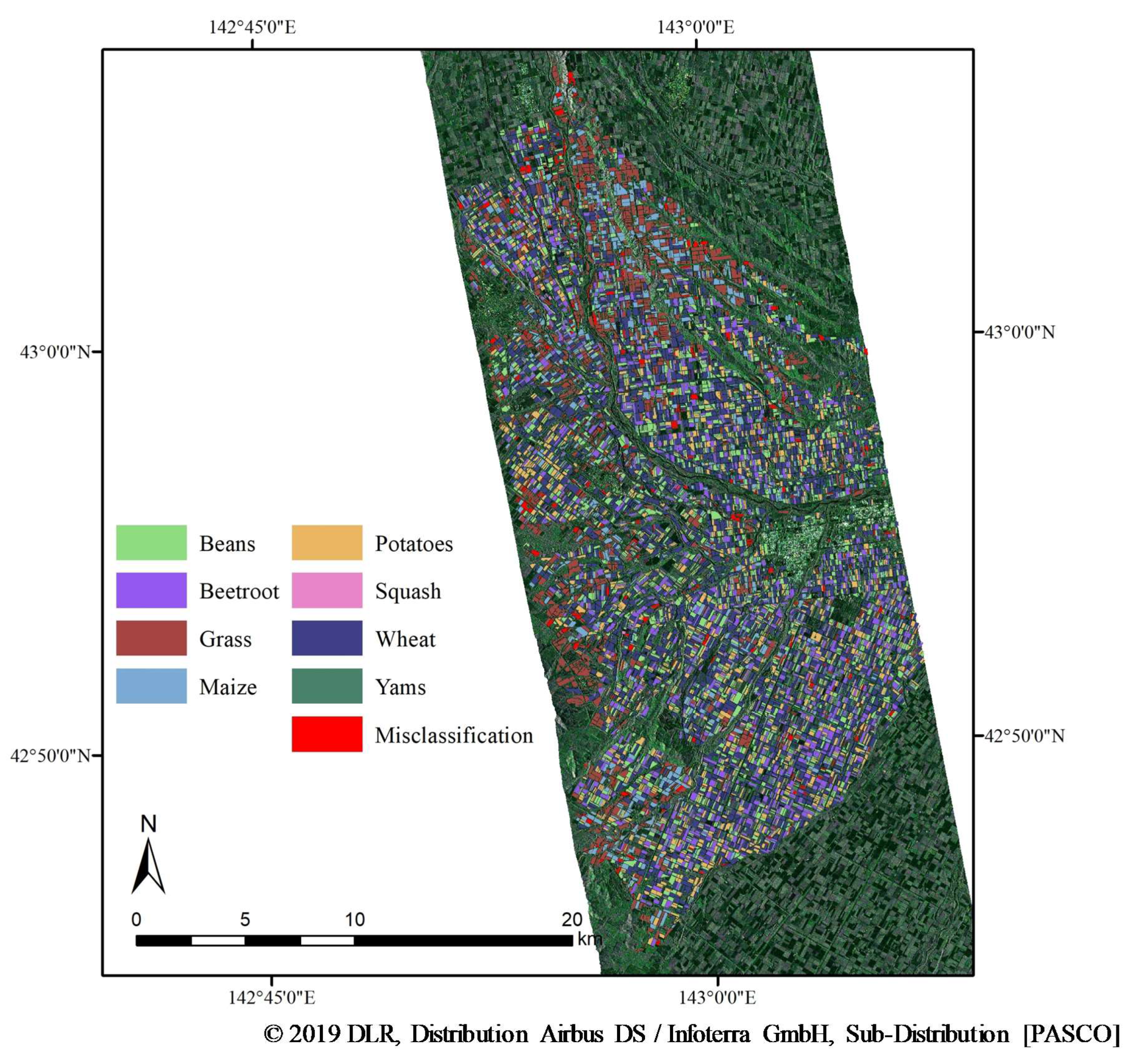
3.3. Accuracy Assessment

The accuracies of the crop classification results, based on 10 repetitions, are shown in Table 5. All algorithms achieved an OA higher than 91.5 % and performed well in classifying the agricultural crops and MKL had the lowest overall AD+QD.
Identification of beetroot, grass, potatoes, and wheat was accurate for all algorithms, and their PA, UA, and F1 scores were higher than 0.9. By contrast, some squash and maize fields were misclassified as beans, and associated accuracies were relatively low since they exhibited similar trends for their predictors and the sample size of the bean fields was the largest. FNN and MKL were somewhat robust in identifying crops whose sample sizes were very small. However, the four other algorithms had PAs less than 0.5 for squash. When the small-sized fields (squash and yam) were ignored and the number of crop types was equal to six, KELM performed more effectively than CART, SVM, RF, and FNN [32,67]. However, the results showed that this algorithm was relatively weak with respect to the addition of small fields. Slight improvements were observed in the identification of squash when the multiple kernel version (MKELM) was applied, but the accuracy was not higher than that observed for SVM and MKL. MKELM also had a poor ability to identify yam fields compared with KELM.

3.4. Statistical Comparison

The McNemar’s test results were used to compare classification accuracies (Table 6). The differences in classification results were significant among the six algorithms (p < 0.05) and MKL, which possessed the lowest overall AD+QD, emerged as the best algorithm for crop classification in this area (Figure 3).

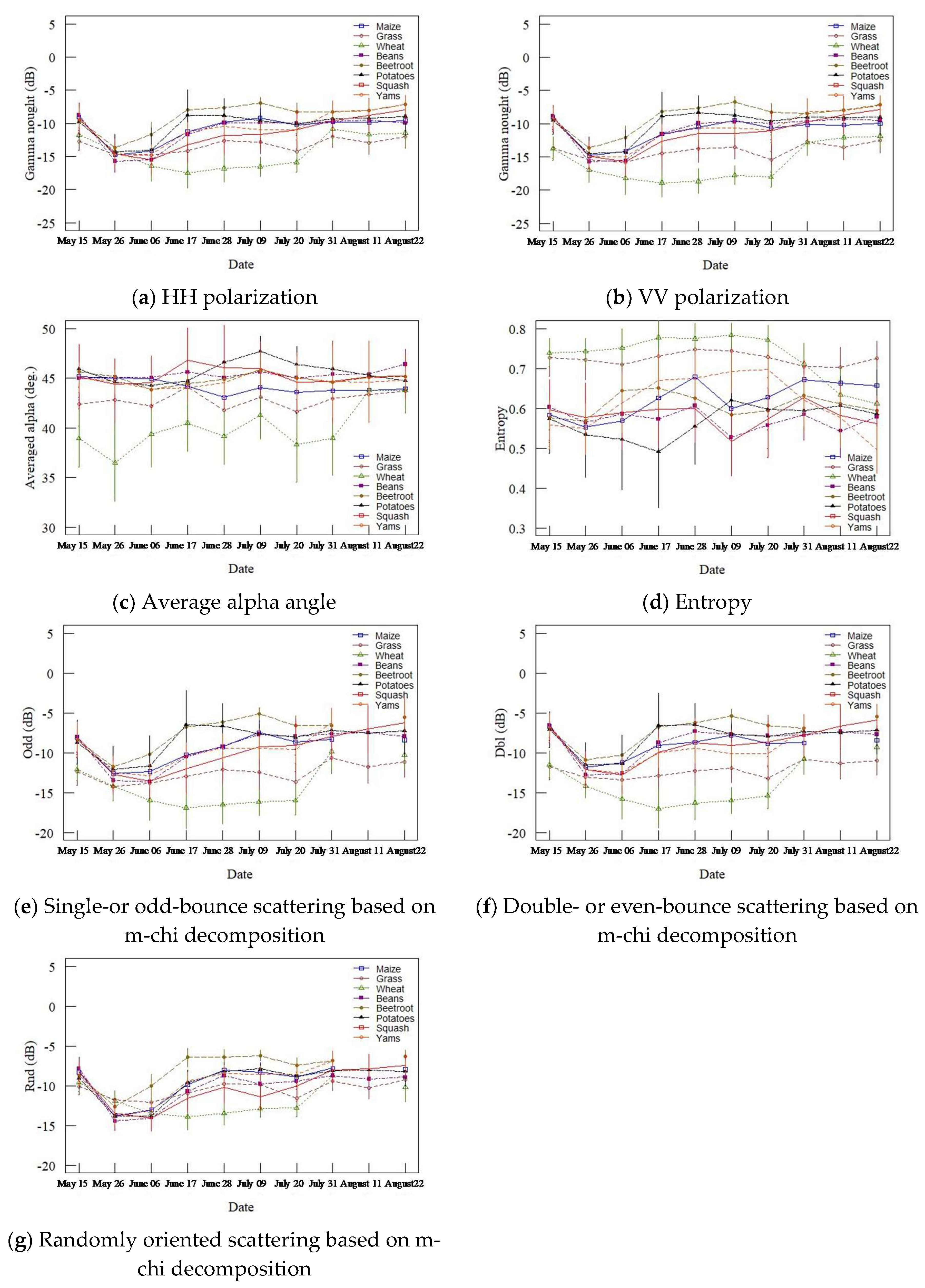
3.5. Sensitivity Analysis

DSA was conducted to clarify which predictors contributed to crop identification within the classification models based on MKL (Figure 4). Although γºVV acquired on 9 July 2013 was the most important metric for identifying wheat fields, Rnd acquired on 28 June 2013 was the most important metric for identifying beans, beetroot, and grassland and the second most important metric for identifying squash, wheat, and yams. On 28 June 2013, which was the start of the growth period for most crops except wheat, the differences in vegetation structure directly influenced the strength of volume scattering from each crop type; the respective highest and lowest Rnd values were confirmed for beetroot, whose rosettes caused efficient backscattering, and wheat, whose structure resulted in microwave absorption. It was easy to observe the differences between crop types due to the different plant heights, except for the combination of maize and potato (Figure 2g). Dbl acquired on 22 August 2013 was another effective m-chi decomposition parameter and was the most important variable to identify squash fields. The contribution of Entropy acquired on 11 August 2013, when beans reached their maximum height and entered the ripening period, and the very small differences in scattering patterns among soy, azuki, and kidney beans, were effective for bean field identification.
The contributions of some RVIs were also confirmed, and the importance of D(Dbl, Odd) acquired on 17 June 2013 was 11.9%, 7.7%, 8.6%, 7.2%, and 4.4% for identifying beans, potato, squash, wheat, and yam fields, respectively. Similarly, the values for ND (Dbl, Rnd) acquired on 6 June 2013 were 14.0% (beetroot) and 8.0% (maize field identification), that for ND (Dbl, Rnd) acquired on 28 June 2013 was 6.5% (for squash), and that for ND (γºHH, Dbl) acquired on 28 June 2013 was 6.4% for wheat.

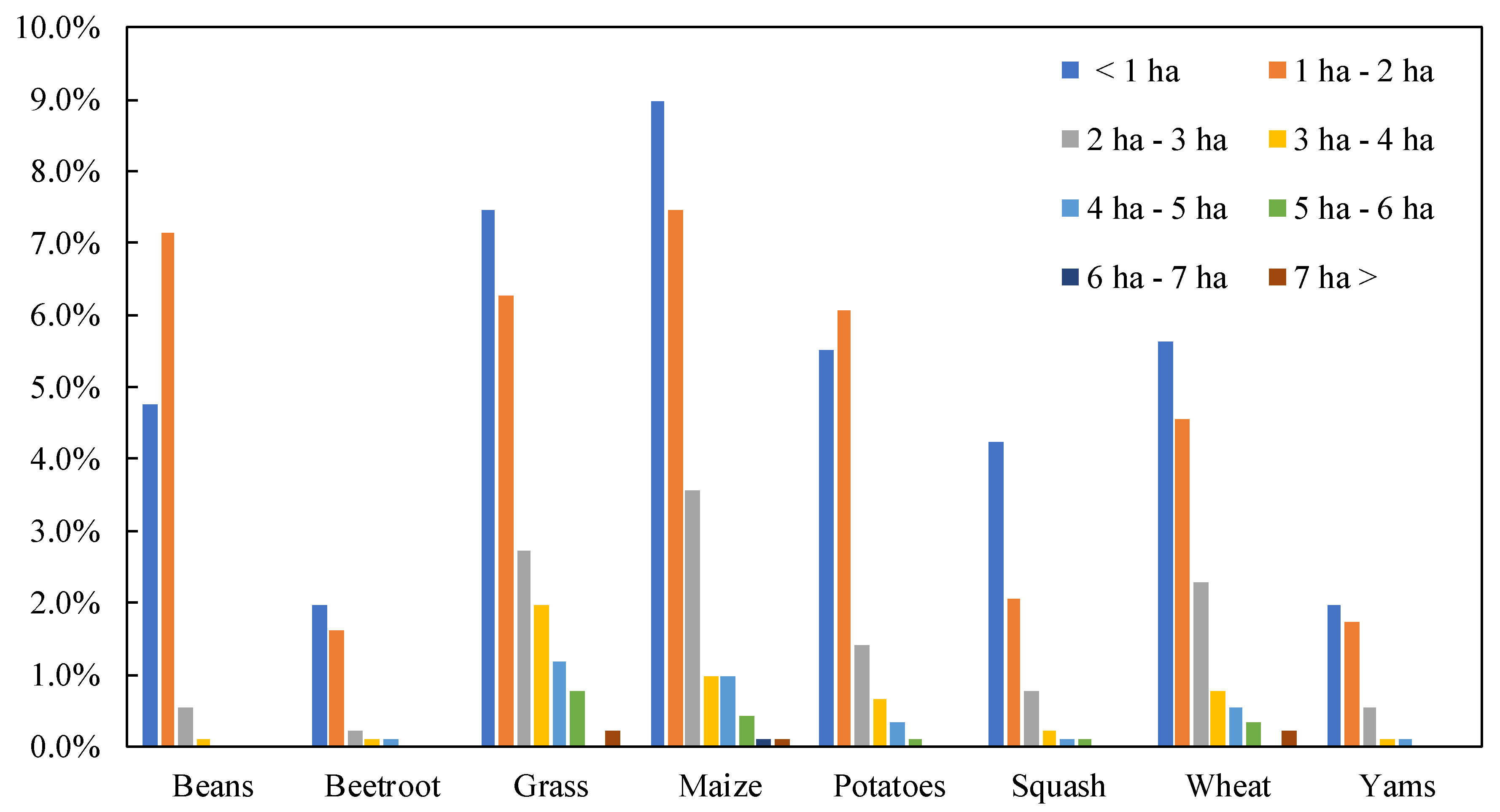
3.6. Relationship between Field Area and Misclassified Fields

Figure 5 shows the relationship between field area and misclassified fields when MKL was applied. In total, 40.5% of the misclassified fields were less than 1 ha, 36.9% were 1–2 ha in area. Therefore, a limitation related to the area of fields could improve the reliability of the classification maps, which could then be particularly effective for identifying grasslands and maize fields. However, smaller fields should not be ignored and some problems related to the borders of fields remain to be resolved. Some studies have shown that the use of a few sets of optical data contributed to the improvement of classification accuracies [32], and future research is planned to evaluate the degree of certainty related to the edges.
Although a few misclassified fields were confirmed to cover an area greater than 5 ha, many grass fields were misclassified since fewer cultivation control methods were employed, and numerous weeds were present in the grasslands.

4. Conclusions

Certain decomposition techniques were applied to TerraSAR-X dual-polarimetric data, and polarimetric parameters were used for crop classification as well as gamma naught values of HH and VV polarization. Furthermore, radar vegetation indices (RVIs), which were calculated from gamma naught values and m-chi decomposition parameters, were also considered. Linear discriminant analysis allowed for the selection of several well-performing RVIs, which can improve classification accuracies. Six types of machine-learning algorithms were tested. While each algorithm achieved an OA value higher than 91.5% and all performed well in classifying agricultural crops, significant differences in classification results were observed. In this study area, the sample sizes of squash and yams fields were very small, occupying ca. 1.2% of the total area; most algorithms failed to identify these crops, especially squash. Of the tested algorithms, multiple kernel learning performed best, achieving an F1 score of 0.62 for the identification of squash fields, as well as an overall accuracy of 92.1%. However, meshing was applied over the yam fields from June and wilting related to chemical treatments was conducted over the potato fields in the study area. Therefore, agricultural practices should be paid attention when the method proposed in this study is handled.

Author Contributions

All analysis and the writing of the paper have been performed by the author.

Funding

This work was supported by JSPS KAKENHI [grant number 19K06313].

Acknowledgments

The authors would like to thank Hiroshi Tani from Hokkaido University, Tokachi Nosai for providing the field data, and the PASCO corporation for providing the TerraSAR-X images.

Conflicts of Interest

The authors declare no conflict of interest.

References

  1. Ministry of Agriculture, Forestry and Fisheries. Available online: http://www8.cao.go.jp/space/comittee/dai36/siryou3-5.pdf (accessed on 1 April 2019).
  2. Demarez, V.; Helen, F.; Marais-Sicre, C.; Baup, F. In-Season Mapping of Irrigated Crops Using Landsat 8 and Sentinel-1 Time Series. Remote Sens. 2019, 11, 118. [Google Scholar] [CrossRef]
  3. Sonobe, R.; Yamaya, Y.; Tani, H.; Wang, X.F.; Kobayashi, N.; Mochizuki, K.I. Evaluating metrics derived from Landsat 8 OLI imagery to map crop cover. Geocarto Int. 2018, 1–17. [Google Scholar] [CrossRef]
  4. Sonobe, R.; Yamaya, Y.; Tani, H.; Wang, X.F.; Kobayashi, N.; Mochizuki, K. Mapping crop cover using multi-temporal Landsat 8 OLI imagery. Int. J. Remote Sens. 2017, 38, 4348–4361. [Google Scholar] [CrossRef] [Green Version]
  5. Liu, J.H.; Zhu, W.Q.; Atzberger, C.; Zhao, A.Z.; Pan, Y.Z.; Huang, X. A Phenology-Based Method to Map Cropping Patterns under a Wheat-Maize Rotation Using Remotely Sensed Time-Series Data. Remote Sens. 2018, 10, 25. [Google Scholar] [CrossRef]
  6. Pan, H.Z.; Chen, Z.X.; Ren, J.Q.; Li, H.; Wu, S.R. Modeling Winter Wheat Leaf Area Index and Canopy Water Content With Three Different Approaches Using Sentinel-2 Multispectral Instrument Data. IEEE J. Sel. Top. Appl. Earth Obs. Remote Sens. 2019, 12, 482–492. [Google Scholar] [CrossRef]
  7. Chemura, A.; Mutanga, O.; Odindi, J. Empirical Modeling of Leaf Chlorophyll Content in Coffee (Coffea Arabica) Plantations with Sentinel-2 MSI Data: Effects of Spectral Settings, Spatial Resolution, and Crop Canopy Cover. IEEE J. Sel. Top. Appl. Earth Obs. Remote Sens. 2017, 10, 5541–5550. [Google Scholar] [CrossRef]
  8. Sonobe, R.; Yamaya, Y.; Tani, H.; Wang, X.F.; Kobayashi, N.; Mochizuki, K. Crop classification from Sentinel-2-derived vegetation indices using ensemble learning. J. Appl. Remote Sens. 2018, 12, 026019. [Google Scholar] [CrossRef]
  9. Ottosen, T.B.; Lommen, S.T.E.; Skjoth, C.A. Remote sensing of cropping practice in Northern Italy using time-series from Sentinel-2. Comput. Electron. Agric. 2019, 157, 232–238. [Google Scholar] [CrossRef]
  10. McNairn, H.; Jiao, X.F.; Pacheco, A.; Sinha, A.; Tan, W.K.; Li, Y.F. Estimating canola phenology using synthetic aperture radar. Remote Sens. Environ. 2018, 219, 196–205. [Google Scholar] [CrossRef]
  11. Sonobe, R.; Tani, H. Application of the Sahebi model using ALOS/PALSAR and 66.3 cm long surface profile data. Int. J. Remote Sens. 2009, 30, 6069–6074. [Google Scholar] [CrossRef] [Green Version]
  12. Gao, Q.; Zribi, M.; Escorihuela, M.J.; Baghdadi, N.; Segui, P.Q. Irrigation Mapping Using Sentinel-1 Time Series at Field Scale. Remote Sens. 2018, 10, 1495. [Google Scholar] [CrossRef]
  13. Amazirh, A.; Merlin, O.; Er-Raki, S.; Gao, Q.; Rivalland, V.; Malbeteau, Y.; Khabba, S.; Escorihuela, M.J. Retrieving surface soil moisture at high spatio-temporal resolution from a synergy between Sentinel-1 radar and Landsat thermal data: A study case over bare soil. Remote Sens. Environ. 2018, 211, 321–337. [Google Scholar] [CrossRef]
  14. Bargiel, D.; Herrmann, S. Multi-temporal land-cover classification of agricultural areas in two European regions with high resolution Spotlight TerraSAR-X data. Remote Sens. 2011, 3, 859–877. [Google Scholar] [CrossRef]
  15. Sonobe, R.; Tani, H.; Wang, X.; Kobayashi, N.; Shimamura, H. Discrimination of crop types with TerraSAR-X-derived information. Phys. Chem. Earth 2015, 83–84, 2–13. [Google Scholar] [CrossRef]
  16. Song, Y.; Wang, J. Mapping Winter Wheat Planting Area and Monitoring Its Phenology Using Sentinel-1 Backscatter Time Series. Remote Sens. 2019, 11, 449. [Google Scholar] [CrossRef]
  17. Xu, L.; Zhang, H.; Wang, C.; Zhang, B.; Liu, M. Crop Classification Based on Temporal Information Using Sentinel-1 SAR Time-Series Data. Remote Sens. 2019, 11, 53. [Google Scholar] [CrossRef]
  18. Park, S.; Im, J.; Yoo, C.; Han, H.; Rhee, J. Classification and Mapping of Paddy Rice by Combining Landsat and SAR Time Series Data. Remote Sens. 2018, 10, 22. [Google Scholar] [CrossRef]
  19. Stendardi, L.; Karlsen, S.R.; Niedrist, G.; Gerdol, R.; Zebisch, M.; Rossi, M.; Notarnicola, C. Exploiting Time Series of Sentinel-1 and Sentinel-2 Imagery to Detect Meadow Phenology in Mountain Regions. Remote Sens. 2019, 11, 542. [Google Scholar] [CrossRef]
  20. Carrasco, L.; O’Neil, A.W.; Morton, R.D.; Rowland, C.S. Evaluating Combinations of Temporally Aggregated Sentinel-1, Sentinel-2 and Landsat 8 for Land Cover Mapping with Google Earth Engine. Remote Sens. 2019, 11, 288. [Google Scholar] [CrossRef]
  21. Santos, C.; Lamparelli, R.A.C.; Figueiredo, G.; Dupuy, S.; Boury, J.; Luciano, A.C.D.; Torres, R.D.; Maire, G. Classification of Crops, Pastures, and Tree Plantations along the Season with Multi-Sensor Image Time Series in a Subtropical Agricultural Region. Remote Sens. 2019, 11, 334. [Google Scholar] [CrossRef]
  22. Bousbih, S.; Zribi, M.; El Hajj, M.; Baghdadi, N.; Lili-Chabaane, Z.; Gao, Q.; Fanise, P. Soil Moisture and Irrigation Mapping in A Semi-Arid Region, Based on the Synergetic Use of Sentinel-1 and Sentinel-2 Data. Remote Sens. 2018, 10, 1953. [Google Scholar] [CrossRef]
  23. Ager, T.P.; Bresnahan, P.C. Geometric precision in space radar imaging: Results from TerraSAR-X. In Proceedings of the ASPRS Annual Conference, Baltimore, ML, USA, 27–31 January 2009; pp. 9–13. [Google Scholar]
  24. Dabrowska-Zielinska, K.; Inoue, Y.; Kowalik, W.; Gruszczynska, M. Inferring the effect of plant and soil variables on C- and L-band SAR backscatter over agricultural fields, based on model analysis. Adv. Space Res. 2007, 39, 139–148. [Google Scholar] [CrossRef]
  25. Blaes, X.; Defourny, P. Retrieving crop parameters based on tandem ERS 1/2 interferometric coherence images. Remote Sens. Environ. 2003, 88, 374–385. [Google Scholar] [CrossRef]
  26. Raney, R.K. Hybrid-polarity SAR architecture. IEEE Trans. Geosci. Remote Sens. 2007, 45, 3397–3404. [Google Scholar] [CrossRef]
  27. Raney, R.K.; Cahill, J.T.S.; Patterson, G.W.; Bussey, D.B.J. The m-chi decomposition of hybrid dual-polarimetric radar data. In Proceedings of the IEEE International Geoscience and Remote Sensing Symposium (IGARSS’12), Munich, Germany, 22–27 July 2012; pp. 5093–5096. [Google Scholar]
  28. Cloude, S.R. The dual polarization entropy/alpha decomposition: A PALSAR case study. In Proceedings of the 3rd International Workshop on Science and Applications of SAR Polarimetry and Polarimetric Interferometry, Frascati, Italy, 22–26 January 2007. [Google Scholar]
  29. Arii, M.; van Zyl, J.J.; Kim, Y. A General Characterization for Polarimetric Scattering From Vegetation Canopies. IEEE Trans. Geosci. Remote Sens. 2010, 48, 3349–3357. [Google Scholar] [CrossRef]
  30. Kim, Y.; Jackson, T.; Bindlish, R.; Lee, H.; Hong, S. Radar Vegetation Index for Estimating the Vegetation Water Content of Rice and Soybean. IEEE Geosci. Remote Sens. Lett. 2012, 9, 564–568. [Google Scholar] [CrossRef]
  31. Hartfield, K.; Marsh, S.; Kirk, C.; Carriere, Y. Contemporary and historical classification of crop types in Arizona. Int. J. Remote Sens. 2013, 34, 6024–6036. [Google Scholar] [CrossRef]
  32. Sonobe, R.; Yamaya, Y.; Tani, H.; Wang, X.F.; Kobayashi, N.; Mochizuki, K.I. Assessing the suitability of data from Sentinel-1A and 2A for crop classification. GISci. Remote Sens. 2017, 54, 918–938. [Google Scholar] [CrossRef]
  33. Foody, G.; Mathur, A. A relative evaluation of multiclass image classification by support vector machines. IEEE Trans. Geosci. Remote Sens. 2004, 42, 1335–1343. [Google Scholar] [CrossRef] [Green Version]
  34. Biau, G.; Scornet, E. A random forest guided tour. Test 2016, 25, 197–227. [Google Scholar] [CrossRef]
  35. Huang, G.B.; Zhou, H.M.; Ding, X.J.; Zhang, R. Extreme learning machine for regression and multiclass classification. IEEE Trans. Syst. Man Cybern. Part B-Cybern. 2012, 42, 513–529. [Google Scholar] [CrossRef]
  36. Sonobe, R.; Sano, T.; Horie, H. Using spectral reflectance to estimate leaf chlorophyll content of tea with shading treatments. Biosyst. Eng. 2018, 175, 168–182. [Google Scholar] [CrossRef]
  37. Sonobe, R.; Miura, Y.; Sano, T.; Horie, H. Monitoring Photosynthetic Pigments of Shade-Grown Tea from Hyperspectral Reflectance. Can. J. Remote Sens. 2018, 44, 104–112. [Google Scholar] [CrossRef]
  38. Pal, M.; Maxwell, A.E.; Warner, T.A. Kernel-based extreme learning machine for remote-sensing image classification. Remote Sens. Lett. 2013, 4, 853–862. [Google Scholar] [CrossRef]
  39. Bengio, Y. Learning deep architectures for ai. Found. Trends Mach. Learn. 2009, 2, 1–127. [Google Scholar] [CrossRef]
  40. LeCun, Y.; Bengio, Y.; Hinton, G. Deep learning. Nature 2015, 521, 436–444. [Google Scholar] [CrossRef] [PubMed]
  41. Gonen, M.; Alpaydin, E. Multiple Kernel Learning Algorithms. J. Mach. Learn. Res. 2011, 12, 2211–2268. [Google Scholar]
  42. Gonen, M.; Alpaydin, E. Localized algorithms for multiple kernel learning. Pattern Recognit. 2013, 46, 795–807. [Google Scholar] [CrossRef]
  43. Liu, X.W.; Wang, L.; Huang, G.B.; Zhang, J.; Yin, J.P. Multiple kernel extreme learning machine. Neurocomputing 2015, 149, 253–264. [Google Scholar] [CrossRef]
  44. Pottier, E.; Ferro-Famil, L.; Allain, S.; Cloude, S.R.; Hajnsek, I.; Papathanassiou, K.; Moreira, A.; Williams, M.; Minchella, A.; Lavalle, M.; et al. Overview of the PolSARpro v4.0: The open source toolbox for polarimetric and interferometric polarimetric SAR data processing. In Proceedings of the IGARSS, Cape Town, South Africa, 12–17 July 2009; pp. 936–939. [Google Scholar]
  45. Gens, R.; Logan, T. Alaska Satellite Facility Software Tools: Manual; Geophysical Institute, University of Alaska: Fairbanks, AK, USA, 2003. [Google Scholar]
  46. Buckreuss, S.; Werninghaus, R.; Pitz, W. The German satellite mission TerraSAR-X. In Proceedings of the IEEE Radar Conference (RadarCon), Rome, Italy, 26–30 May 2008; pp. 1–5. [Google Scholar]
  47. Betbeder, J.; Fieuzal, R.; Philippets, Y.; Ferro-Famil, L.; Baup, F. Contribution of multitemporal polarimetric synthetic aperture radar data for monitoring winter wheat and rapeseed crops. J. Appl. Remote Sens. 2016, 10, 19. [Google Scholar] [CrossRef]
  48. Phalke, A.R.; Ozdogan, M. Large area cropland extent mapping with Landsat data and a generalized classifier. Remote Sens. Environ. 2018, 219, 180–195. [Google Scholar] [CrossRef]
  49. Roever, C.; Raabe, N.; Luebke, K.; Ligges, U.; Szepannek, G.; Zentgraf, M. Classification and Visualization. Available online: https://cran.r-project.org/web/packages/klaR/klaR.pdf (accessed on 12 December 2018).
  50. Raschka, S. Linear Discriminant Analysis Bit by Bit. Available online: https://sebastianraschka.com/Articles/2014_python_lda.html (accessed on 1 April 2019).
  51. Hastie, T.; Tibshirani, R.; Friedman, J. The Elements of Statistical Learning: Data Mining, Inference, and Prediction, 2nd ed.; Springer: New York, NY, USA, 2009; p. 745. [Google Scholar]
  52. R core team R: A Language and Environment for Statistical Computing. R Foundation for Statistical Computing. Available online: https://www.R-project.org/ (accessed on 1 April 2019).
  53. Ghosh, A.; Fassnacht, F.E.; Joshi, P.K.; Koch, B. A framework for mapping tree species combining hyperspectral and LiDAR data: Role of selected classifiers and sensor across three spatial scales. Int. J. Appl. Earth Obs. Geoinf. 2014, 26, 49–63. [Google Scholar] [CrossRef]
  54. Svozil, D.; Kvasnicka, V.; Pospichal, J. Introduction to multi-layer feed-forward neural networks. Chemom. Intell. Lab. Syst. 1997, 39, 43–62. [Google Scholar] [CrossRef]
  55. Huang, G.B.; Zhu, Q.Y.; Siew, C.K. Extreme learning machine: Theory and applications. Neurocomputing 2006, 70, 489–501. [Google Scholar] [CrossRef] [Green Version]
  56. Puertas, O.; Brenning, A.; Meza, F. Balancing misclassification errors of land cover classification maps using support vector machines and Landsat imagery in the Maipo river basin (Central Chile, 1975–2010). Remote Sens. Environ. 2013, 137, 112–123. [Google Scholar] [CrossRef]
  57. Bergstra, J.; Bengio, Y. Random Search for Hyper-Parameter Optimization. J. Mach. Learn. Res. 2012, 13, 281–305. [Google Scholar]
  58. Snoek, J.; Rippel, O.; Swersky, K.; Kiros, R.; Satish, N.; Sundaram, N.; Patwary, M.M.A.; Prabhat; Adams, R.P. Scalable Bayesian optimization using deep neural networks. In Proceedings of the 32nd International Conference on Machine Learning (ICML), Paris, France, 6–11 July 2015; pp. 2171–2180. [Google Scholar]
  59. Cusano, C.; Napoletano, P.; Schettini, R. Remote Sensing Image Classification Exploiting Multiple Kernel Learning. IEEE Geosci. Remote Sens. Lett. 2015, 12, 2331–2335. [Google Scholar] [CrossRef]
  60. Zamani, F.; Jamzad, M. A feature fusion based localized multiple kernel learning system for real world image classification. EURASIP J. Image Video Process. 2017, 78. [Google Scholar] [CrossRef]
  61. Pontius, R.; Millones, M. Death to Kappa: Birth of quantity disagreement and allocation disagreement for accuracy assessment. Int. J. Remote Sens. 2011, 32, 4407–4429. [Google Scholar] [CrossRef]
  62. McNemar, Q. Note on the sampling error of the difference between correlated proportions or percentages. Psychometrika 1947, 12, 153–157. [Google Scholar] [CrossRef] [PubMed]
  63. Congalton, R.G.; Green, K. Assessing the Accuracy of Remotely Sensed Data: Principles and Practices; CRC Press: Boca Raton, FL, USA, 2008. [Google Scholar]
  64. Benjankar, R.; Glenn, N.F.; Egger, G.; Jorde, K.; Goodwin, P. Comparison of field-observed and simulated map output from a dynamic floodplain vegetation model using remote sensing and GIS techniques. GISci. Remote Sens. 2010, 47, 480–497. [Google Scholar] [CrossRef]
  65. Cortez, P.; Embrechts, M.J. Using sensitivity analysis and visualization techniques to open black box data mining models. Inf. Sci. 2013, 225, 1–17. [Google Scholar] [CrossRef] [Green Version]
  66. Fontanelli, G.; Paloscia, S.; Zribi, M.; Chahbi, A. Sensitivity analysis of X-band SAR to wheat and barley leaf area index in the Merguellil Basin. Remote Sens. Lett. 2013, 4, 1107–1116. [Google Scholar] [CrossRef] [Green Version]
  67. Sonobe, R.; Tani, H.; Wang, X.F. An experimental comparison between KELM and CART for crop classification using Landsat-8 OLI data. Geocarto Int. 2017, 32, 128–138. [Google Scholar] [CrossRef]
Figure 1. Study area and TerraSAR-X data acquired on July 20, 2013 (Red: odd-bounce, Green: randomly oriented, Blue: double-bounce scattering components calculated from m-chi decomposition).
Remotesensing 11 01148 g001
Figure 2. Temporal variation of TerraSAR-X data: gamma naught values of (a) HH, (b) VV polarization; (c) average alpha angle and (d) entropy based on the dual polarization entropy/alpha decomposition; (e) single- or odd-bounce, (f) double- or even-bounce; and (g) randomly oriented scattering based on m-chi decomposition.
Remotesensing 11 01148 g002
Figure 3. Crop classification map based on MKL. Red-colored fields were misclassified.
Remotesensing 11 01148 g003
Figure 4. The data-based sensitivity analysis (DSA) results for each crop type.
Remotesensing 11 01148 g004
Figure 5. The relationship between field area and misclassified fields.
Remotesensing 11 01148 g005
Table 1. The cultivation calendar for crops.
MayJuneJulyAugustSeptemberOctober
midlateearlymidlateearlymidlateearlymidlateearlymidlateearlymidlate
BeansSowing Sprouting Harvesting
Beetroot Transplanting Harvesting
Grass Appearance of ears of grain1st Harvesting 2nd Harvesting
Maize Sowing Sprouting Appearance of ears of grain Harvesting
Potatoes Sowing Sprouting Harvesting
Squash Transplanting Harvesting
Wheat Appearance of ears of grain Harvesting Sowing
Yams Sowing Netting Harvesting
Table 2. Characteristics of the satellite data.
SatelliteAcquisition DateModeIncidence Angle (°)Orbit CyclePass Direction
NearFar
TerraSAR-X15 May 2013StripMap41.736 42.977 197Ascending
TerraSAR-X26 May 2013StripMap41.734 42.975 198Ascending
TerraSAR-X6 June 2013StripMap41.739 42.979 199Ascending
TerraSAR-X17 June 2013StripMap41.737 42.976 200Ascending
TerraSAR-X28 June 2013StripMap41.733 42.973 201Ascending
TerraSAR-X9 July 2013StripMap41.738 42.977 202Ascending
TanDEM-X20 July 2013StripMap41.712 42.952 203Ascending
TerraSAR-X31 July 2013StripMap41.737 42.977 204Ascending
TanDEM-X11 August 2013StripMap41.730 42.971 205Ascending
TanDEM-X22 August 2013StripMap41.737 42.978 206Ascending
Table 3. Crop type and number of fields.
Training DataValidation DataTest Data
Beans942471471
Beetroot713356357
Grass722361362
Maize546273273
Potatoes782391391
Squash653333
Wheat1517759759
Yams673434
Table 4. Selected predictors based on linear discriminant analysis (LDA).
RoundSelected Predictors
1γºVV_May26γºVV_July09γºVV_July20EntropyAugust11RndJune28DblAugust22
ND(γºVV, Dbl)May15ND(Dbl, Rnd)June06ND(Odd, Rnd)June17ND(γºHH, Dbl)June28
2γºVV_May26γºVV_July09EntropyAugust11RndJune28DblAugust22D(Dbl, Odd)June17
ND(γºHH, γºVV)May26ND(Dbl, Rnd)June06ND(γºVV, Dbl)June28
3γºVV_May26γºVV_July09EntropyAugust11RndJune28DblAugust22D(Dbl, Odd)June17
ND(Dbl, Rnd)June06ND(γºHH, Dbl)June28ND(γºHH, γºVV)July20
4γºVV_May26γºVV_July09EntropyAugust11RndJune28DblAugust22D(Dbl, Odd)June17
ND(γºVV, Dbl)May15ND(Dbl, Rnd)June06ND(γºVV, Dbl)June28
5γºVV_May26γºVV_July09RndJune28DblAugust22D(Dbl, Odd)June17ND(γºVV, Odd)June06
ND(Dbl, Rnd)June06ND(γºHH, Dbl)June28ND(Dbl, Rnd)June28
6γºVV_May26γºVV_July09γºVV_July20RndJune28RndJuly31SR(γºHH, γºVV)July20
D(Dbl, Odd)June17ND(Dbl, Rnd)June06ND(Dbl, Rnd)June28ND(γºVV, Rnd)August22
7γºVV_May26γºVV_July09γºVV_July20EntropyAugust11RndJune28RndJuly09
DblAugust22ND(Dbl, Rnd)June06ND(Odd, Rnd)June17ND(γºHH, Dbl)June28ND(γºHH, γºVV)July09
8γºVV_May26γºVV_July09γºVV_July20EntropyAugust11RndJune28DblAugust22
D(Dbl, Odd)June17ND(Dbl, Rnd)June06ND(γºHH, Dbl)June28
9γºVV_May26γºVV_July09EntropyAugust11RndJune28DblAugust22D(Dbl, Odd)June17
ND(Dbl, Rnd)June06ND(γºVV, Dbl)June28
10γºVV_May26γºVV_July09EntropyAugust11RndJune28DblAugust22D(Dbl, Odd)June17
ND(Dbl, Rnd)June06ND(γºVV, Dbl)June28
Table 5. Accuracy results for six classification algorithms: support vector machine (SVM), random forest (RF), multilayer feedforward neural network (FNN), kernel-based extreme learning machine (KELM), multiple kernel learning (MKL), and multiple kernel extreme learning machine (MKELM). PA: producer accuracy; UA: user accuracy; OA: overall accuracy; AD: allocation disagreement; QD: quantity disagreement.
SVMRFFNNKELMMKLMKELM
PA
Beans0.928 ± 0.019 0.920 ± 0.021 0.924 ± 0.020 0.931 ± 0.020 0.925 ± 0.012 0.931 ± 0.019
Beetroot0.966 ± 0.008 0.966 ± 0.008 0.963 ± 0.009 0.968 ± 0.009 0.966 ± 0.009 0.968 ± 0.009
Grass0.901 ± 0.019 0.903 ± 0.019 0.910 ± 0.024 0.897 ± 0.024 0.905 ± 0.015 0.896 ± 0.025
Maize0.827 ± 0.023 0.814 ± 0.027 0.823 ± 0.042 0.819 ± 0.020 0.825 ± 0.018 0.814 ± 0.020
Potatoes0.923 ± 0.018 0.913 ± 0.011 0.915 ± 0.024 0.929 ± 0.019 0.925 ± 0.018 0.931 ± 0.017
Squash0.479 ± 0.097 0.397 ± 0.042 0.500 ± 0.091 0.355 ± 0.082 0.573 ± 0.069 0.464 ± 0.069
Wheat0.964 ± 0.007 0.964 ± 0.007 0.955 ± 0.011 0.962 ± 0.009 0.961 ± 0.010 0.965 ± 0.010
Yams0.747 ± 0.067 0.671 ± 0.081 0.774 ± 0.061 0.674 ± 0.056 0.788 ± 0.046 0.579 ± 0.083
UA
Beans0.894 ± 0.013 0.895 ± 0.015 0.897 ± 0.026 0.887 ± 0.012 0.902 ± 0.015 0.895 ± 0.009
Beetroot0.964 ± 0.008 0.960 ± 0.010 0.969 ± 0.014 0.960 ± 0.012 0.964 ± 0.011 0.959 ± 0.011
Grass0.889 ± 0.013 0.880 ± 0.016 0.870 ± 0.019 0.887 ± 0.008 0.892 ± 0.013 0.885 ± 0.010
Maize0.843 ± 0.026 0.812 ± 0.023 0.844 ± 0.028 0.851 ± 0.018 0.849 ± 0.023 0.855 ± 0.020
Potatoes0.916 ± 0.014 0.907 ± 0.016 0.916 ± 0.036 0.909 ± 0.016 0.919 ± 0.010 0.901 ± 0.018
Squash0.786 ± 0.075 0.829 ± 0.106 0.740 ± 0.076 0.785 ± 0.089 0.700 ± 0.152 0.869 ± 0.105
Wheat0.969 ± 0.009 0.968 ± 0.006 0.972 ± 0.012 0.965 ± 0.011 0.973 ± 0.006 0.963 ± 0.012
Yams0.836 ± 0.087 0.844 ± 0.076 0.745 ± 0.117 0.871 ± 0.052 0.813 ± 0.152 0.916 ± 0.069
F1
Beans0.911 ± 0.012 0.908 ± 0.012 0.910 ± 0.013 0.909 ± 0.010 0.913 ± 0.010 0.913 ± 0.010
Beetroot0.965 ± 0.006 0.963 ± 0.007 0.966 ± 0.007 0.964 ± 0.009 0.965 ± 0.008 0.963 ± 0.008
Grass0.895 ± 0.010 0.891 ± 0.012 0.890 ± 0.008 0.892 ± 0.010 0.898 ± 0.011 0.890 ± 0.010
Maize0.835 ± 0.021 0.813 ± 0.015 0.834 ± 0.017 0.835 ± 0.015 0.836 ± 0.015 0.834 ± 0.016
Potatoes0.919 ± 0.010 0.910 ± 0.005 0.915 ± 0.010 0.919 ± 0.009 0.922 ± 0.007 0.916 ± 0.008
Squash0.595 ± 0.062 0.537 ± 0.042 0.597 ± 0.070 0.489 ± 0.086 0.620 ± 0.065 0.605 ± 0.066
Wheat0.967 ± 0.005 0.966 ± 0.004 0.963 ± 0.006 0.963 ± 0.005 0.967 ± 0.006 0.964 ± 0.005
Yams0.789 ± 0.060 0.748 ± 0.066 0.759 ± 0.075 0.760 ± 0.048 0.794 ± 0.085 0.710 ± 0.064
OA0.921 ± 0.004 0.915 ± 0.004 0.918 ± 0.004 0.918 ± 0.004 0.921 ± 0.005 0.919 ± 0.005
AD0.066 ± 0.007 0.070 ± 0.006 0.062 ± 0.004 0.064 ± 0.008 0.067 ± 0.005 0.062 ± 0.007
QD0.013 ± 0.005 0.015 ± 0.005 0.021 ± 0.006 0.018 ± 0.004 0.012 ± 0.004 0.019 ± 0.003
AD+QD0.079 ± 0.004 0.085 ± 0.004 0.082 ± 0.004 0.082 ± 0.004 0.078 ± 0.003 0.081 ± 0.005
Table 6. Chi-square values from McNemar’s test performed on the six classification algorithms. A chi-square value ≥ 3.84 indicates a significant difference (p < 0.05) between two classification results.
SVMRFFNNKELMMKL
RF30.84 ± 5.26 55.78 ± 14.63 61.36 ± 13.62 43.55 ± 13.50 45.78 ± 11.57
FNN59.14 ± 15.38 31.85 ± 7.45 62.30 ± 14.36 24.76 ± 9.40
KELM31.25 ± 10.89 41.89 ± 8.59 67.10 ± 17.21
MKL35.54 ± 10.39 33.91 ± 8.10
MKELM36.76 ± 9.63

