Abstract
Land-cover monitoring is one of the core applications of remote sensing. Monitoring and mapping changes in the distribution of agricultural land covers provide a reliable source of information that helps environmental sustainability and supports agricultural policies. Synthetic Aperture Radar (SAR) can contribute considerably to this monitoring effort. The first objective of this research is to extend the use of time series of polarimetric data for land-cover classification using a decision tree classification algorithm. With this aim, RADARSAT-2 (quad-pol) and Sentinel-1 (dual-pol) data were acquired over an area of 600 km2 in central Spain. Ten polarimetric observables were derived from both datasets and seven scenarios were created with different sets of observables to evaluate a multitemporal parcel-based approach for classifying eleven land-cover types, most of which were agricultural crops. The study demonstrates that good overall accuracies, greater than 83%, were achieved for all of the different proposed scenarios and the scenario with all RADARSAT-2 polarimetric observables was the best option (89.1%). Very high accuracies were also obtained when dual-pol data from RADARSAT-2 or Sentinel-1 were used to classify the data, with overall accuracies of 87.1% and 86%, respectively. In terms of individual crop accuracy, rapeseed achieved at least 95% of a producer’s accuracy for all scenarios and that was followed by the spring cereals (wheat and barley), which achieved high producer’s accuracies (79.9%-95.3%) and user’s accuracies (85.5% and 93.7%).
Keywords:
agriculture; classification; C5.0 algorithm; multitemporal; polarimetric SAR; RADARSAT-2; Sentinel-1 1. Introduction
Land-cover classification on different scales provides accurate and cost-effective information whilst representing an important asset for various applications, from environment to economy. Knowing the crop present on each agricultural field on national and regional scales is valuable information for crop yield forecasting [1] and crop area estimation [2]. On a global scale, the knowledge of cropland uses and covers is key for estimating global food production or drought risk analysis and can even have an impact on studies on climate events and water [3].
Remote sensing is an effective and reliable data source for classifying different land covers. Optical remote sensing images have demonstrated that vegetation types can be clearly distinguished by exploiting their spectral signature and the phenological stage at the time of the image acquisition. However, due to the presence of clouds, optical remote sensing images can miss crucial periods in the growing season, thus they may not be accurate enough for crop classification in some situations [4].
However, active microwave sensors can provide data independently from daylight, cloud cover and weather conditions, making Synthetic Aperture Radar (SAR) images relevant to agricultural applications, such as crop classification and monitoring activities, that are time-critical. In addition, early studies reported that SAR images could be integrated with optical satellite images to achieve very high crop classification accuracies, for example, using C-band images with at least one optical image [5,6,7,8,9].
Since the launch of the ERS-1 (European Remote Sensing Satellite) by the European Space Agency (ESA) in 1991, several SAR sensors have been developed with different frequencies and polarizations. Radar sensitivity depends on the frequency band and on the polarization of the waves. Regarding the frequency, the lower the frequency, the farther the waves penetrate; therefore, lower frequencies are more sensitive to the ground conditions, whereas high frequencies have a shallower penetration capacity and are more sensitive to the vegetation canopy. C-band-based sensors (~5.4 GHz) are on board satellites such as RADARSAT-1 and -2, RISAT-1 (Radar Imaging Satellite), ENVISAT/ASAR (Environmental Satellite/Advanced Synthetic Aperture Radar) and more recently Sentinel-1 [10] as part of Copernicus, the European Commission’s Earth Observation Programme [11]. Other sensors operate at L-band (~1.3 GHz), such as in JERS-1 (Japanese Earth Resource Satellite) and ALOS/PALSAR-1 and -2 (Advanced Land Observing Satellite); whereas X-band sensors (~10 GHz) are on board TerraSAR-X, TanDEM-X and COSMO-SkyMed. In addition to the frequency, radar sensitivity depends also on the polarimetric configuration. Polarimetry is sensitive to the geometry or morphology of the plants, so different polarimetric channels present different responses as a function of the geometrical properties of the scene. Thus, some of the satellites operate in dual-pol mode and a few in quad-pol configurations.
In the field of crop discrimination and land-cover classification, a multifrequency multipolarization data set would be a useful option. Compared to single frequency data, researchers reported higher classification accuracies with C-, L- and P-band data [12,13,14]. The advantage of multifrequency data sets for separating vegetation types has also been demonstrated using data acquired from multiple satellite platforms, especially ERS (C-band) and JERS (L-band) [15,16]. As mentioned above, lower frequencies (i.e., L-band) penetrate larger biomass crops and the scattering within the canopy, where structure is quite different, helps in separating them [17]. For smaller biomass canopies, lower frequencies can penetrate too far into the canopy and become mostly dependent on soil properties such as the soil moisture content [18]. In this case, discrimination is achieved using higher frequency microwaves where most interaction is limited to the canopy. In addition, a distinct variation is seen for the agricultural scene properties due to the development of crops through the growing season [19]. Therefore, the discrimination capabilities may vary through the year, and, consequently, land-cover mapping can be significantly improved by performing a multitemporal classification [9,20,21,22]. Multitemporal image classification not only improves the overall accuracy of classifier but also provides more reliable crop discrimination in comparison to single-date [23,24,25,26,27].
Regardless of the sensor or frequency used, a key to successful crop classification lies in understanding which growth stages are best for crop discrimination. Like optical sensors, the energy recorded by SAR sensors could be similar for different crops at a given point in their growing cycle. However, the use of multitemporal datasets allows us to distinguish more crops from each other due to their different phenological cycles [23,28,29].
With the increasing number of spaceborne SAR systems, different SAR techniques, such as polarimetry (PolSAR), interferometry (InSAR) and differential interferometry (DInSAR), have also increased their abilities to improve parameter retrieval (e.g., biophysical variables), derive surface topography (e.g., digital elevation models (DEMs)) and measure the Earth’s surface displacement, respectively. SAR polarimetry has been widely used as a technique for obtaining qualitative and quantitative physical information over land. Regarding land cover classification, instead of approaching the classification problem with simply one single-polarization single-date single-frequency input image, the enlargement of the observation space by adding diversity is highly beneficial, as it is described in many examples in the literature and briefly reviewed here.
Regarding the use of individual polarization, many studies have confirmed that the cross-polar channel (HV or VH, which are virtually identical due to reciprocity) is the most important single polarization to identify the majority of crops [8,17,30,31,32]. This polarization is responsive to multiple scattering from the vegetation volume and since vegetation structures vary greatly among vegetation canopies, the cross-polarized backscatter provides the best discrimination. Nevertheless, classification accuracy is increased substantially with the inclusion of additional polarimetric channels in form of backscattering coefficients or other alternative ways (e.g., other derived observables or different matrix forms of the radar data). Regarding the use of backscattering coefficients of more than one polarimetric channel, a significant improvement in accuracy is observed when adding a second channel [31], whereas a third polarization results in extra improvements in classification accuracy only for specific crops [8].
The exploitation of polarimetric SAR data for crop classification is usually carried out by employing the covariance or coherency matrices but additional different approaches exist [22]: 1) statistical methods based on the Wishart distribution of the data; 2) transformation of covariance matrix entries into backscatter-like coefficients; 3) methods based on scattering mechanisms; and 4) knowledge-based methods. It is possible to apply relatively robust methods and easily adjust to different growing conditions [21], including both the results of the scattering model and common knowledge about targets. However, these methods have the disadvantage of only being able to determine a relatively small number of classes. The contribution of polarimetry was also assessed in Reference [33] by testing the performance when input information is removed progressively. The capability of polarimetric SAR data in crop classification has also been demonstrated by applying machine learning algorithms such as Random Forest (RF) [34,35,36], Decision Tree (DT) [37,38], Neural Networks (NNs) [39] and Support Vector Machines (SVMs) [40,41].
The present research is aimed at extending the use of a time series of polarimetric observables for land-cover classification, mainly focussed over agricultural fields. This possibility was previously identified [42] when several crop parameters were tested against radar measurements. The difference found in the correlations for different crop types suggested that specific crops, mainly cereal types, could be classified using SAR observables. Here, the set of land-cover types is enlarged with other vegetation types, including vineyard and forest. With this aim, we exploited a total of 20 RADARSAT-2 images acquired at three different incidence angles, as well as 14 Sentinel-1A images that were acquired during the growing season of 2015 over an agricultural area of 600 km2 in central Spain. Different SAR observables were derived from each dataset and a parcel-based classification was performed using a decision tree classifier. The main objectives of this study were: 1) the evaluation of different polarimetric observables for land cover classification in a multitemporal approach, 2) the assessment and comparison of dual- and quad-polarimetric SAR data from different sensors for classification and 3) the analysis of the influence of the incidence angle for classification.
2. Materials and Methods
2.1. Study Area and Ground Truth
The study area is located in central Spain and covers an area of approximately 35 km x 18 km in the Castilla y Leon region (Figure 1). The topography of the study area is characterized by flat areas with slopes of up to 12%. The climate is continental semiarid Mediterranean characterized by dry and warm summers and cool to mild and wet winters. The limited amount of rainfall (336 mm average over the last 10 years) together with the shallow soils make this area prone to rainfed crops, mainly cereals and industrial crops (sunflower and rapeseed).
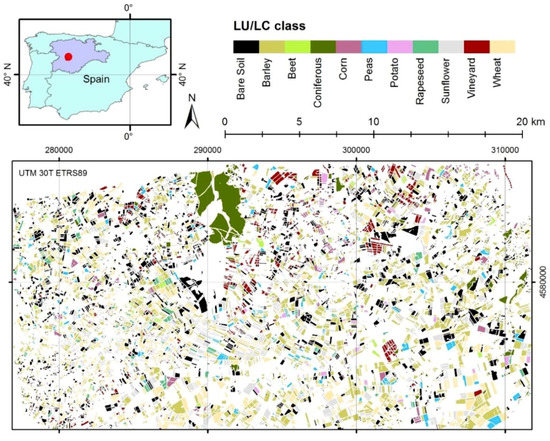
Figure 1.
Study area and selected plots, indicating their land use/land cover (LU/LC) category from the map.
Both to train the classification and to assess the accuracy of the resulting classification maps, a land-use/land-cover (LU/LC) map of the whole Castilla y Leon region from 2015 was used as the ground truth of the LU/LC for each plot. Since 2011, the Agriculture Technological Institute of Castilla y Leon (ITACyL) map service (http://mcsncyl.itacyl.es/en/descarga) has updated the LU/LC maps annually. These maps are based on optical image classification and represent the changes in annual arable crops as well as permanent crops and natural vegetation areas. Their spatial resolution is 20 m. The overall classification accuracy of these maps is 82% on average (kappa coefficient around 0.78), which is generally much higher for crop categories than for natural land [43].
Based on the LU/LC map for 2015 and field surveys, the selected crops to be classified were: wheat (Triticum aestivum L.), sunflower (Helianthus annuus L.), barley (Hordeum vulgare L.), peas (Pisum sativum L.), rapeseed (Brassica napus L.), corn (Zea mays L.), beet (Beta vulgaris L.), potatoes (Solanum tuberosum L.) and vineyards (Vitis vinifera), as well as two other covers: bare soil and coniferous. The growing season of these crops can be clustered into two groups: long cycle, from fallow to the end of the spring (wheat, barley, peas and rapeseed) and short cycle, from spring to the beginning of fallow (sunflower, corn, beet and potatoes). Vineyard and coniferous are permanent covers.
Table 1 shows the number of plots (total 7580) and their area on average; their geographical distribution is shown in Figure 1. For classification purposes, 60% of the plots were selected randomly as the training dataset and 40% as the validation dataset. Prior to classification and to avoid selecting training pixels from the field boundaries, the plots of the training dataset were buffered inward by 20 m, following the approach of Sonobe et al. [40].

Table 1.
Overview of ground truth data.
2.2. RADARSAT-2 and Sentinel-1A Data
RADARSAT-2 and Sentinel-1 data were used for crop classification over the study area, using data acquired between February and July 2015. RADARSAT-2, launched by the Canadian Space Agency (CSA) and MacDonald, Dettwiler and Associates Ltd. (MDA) in December 2007, has a C-band (5.405 GHz) SAR sensor and multiple beam modes, with an orbit repeat cycle of 24 days. Sentinel-1A is the first of the two Sentinel-1 satellites. It was launched in April 2014 by ESA. It operates at C-band (5.405 GHz) with an orbit repeat cycle of 12 days and it has four different operational modes—Interferometric Wide Swath (IW), Wave (WV), Stripmap (SM) and Extra Wide Swath (EW). All modes are available in single (HH or VV) or dual polarization (HH and HV or VV and VH), except for WV, which is available just in single polarization [10].
For the purpose of this study, three sets of Fine Quad-Pol RADARSAT-2 Single Look Complex (SLC) images at different incidence angles were acquired. The Fine Quad-Pol mode provides a high spatial resolution and the capacity to extract polarimetric observables. From Sentinel-1A, we obtained high resolution Level-1 IW Ground Range Detected (GRD) dual-polarization (VV and VH) images. According to the product specifications, Level-1 GRD products have already been detected, multi-looked and projected to the ground range using an Earth ellipsoid model. Some basic information about RADARSAT-2 and Sentinel-1A images, as well as a list of the available acquisition data, are shown in Table 2; Table 3, respectively.
Table 2.
Characteristics of RADARSAT-2 and Sentinel-1A.
Table 3.
List of RADARSAT-2 and Sentinel-1A IW ground range detected (GRD) images.
2.3. SAR Data Processing
Some steps were applied to pre-process RADARSAT-2 and Sentinel-1A images. Both datasets were pre-processed using free-access Sentinel-1 Toolbox of the SNAP (Sentinel Application Platform) software provided by ESA.
The steps applied to RADARSAT-2 images were as follows: 1) radiometric calibration to sigma naught backscatter values; 2) polarimetric coherency matrix generation [44]; 3) application of a spatial average speckle filter to the coherency matrix (a 9x9 boxcar filter was selected); 4) terrain correction and geocoding using the Range Doppler orthorectification method available in SNAP and the digital elevation model from the Shuttle Radar Topography Mission; and 5) polarimetric observables computation using the free-access PolSARpro software provided by ESA. In total, 10 polarimetric observables (Table 4) were derived from the input polarimetric RADARSAT-2 SAR data. The symbols used hereafter to denote these observables are shown in Table 4.
Table 4.
List of polarimetric observables derived from RADARSAT-2.
Pre-processing Sentinel-1A images consisted of: 1) precise orbit ephemerides files were used for the geolocation accuracy [45]; 2) data calibration to obtain the sigma naught (σ0) backscatter coefficient; 3) terrain correction and geocoding using the Range Doppler orthorectification method available in SNAP and the digital elevation model from the Shuttle Radar Topography Mission; 4) a temporal stack using the first image as master; 5) application of a multitemporal speckle filter to reduce the speckle effect without degrading the spatial resolution of GRD data at 10 m; and 6) transformation of the terrain-corrected backscatter coefficients of VV and VH to dB scale and derivation of the ratio between both channels (subtraction in dB).
2.4. Classification Algorithm
The See5 or C5.0 decision tree (DT) classification algorithm was used for this study. The reason for using this software and DT is that DTs have proven to be consistent and reliable with SAR data used in crop classification [8,17].
C5.0 is based on decision trees and was developed from the well-known and widely used C4.5 algorithm [46]. DTs are non-parametric methods, which can be used for both classification and regression. DTs predict class membership by dividing data sets into progressively homogeneous and mutually exclusive subsets via a branched system of data splits. A DT is composed of internal nodes (decision or rules applied), branches (connections linking two nodes) and terminal nodes (leaves), which represent the class labels. Given an input (i.e., training samples) at each internal node, they split the data set into subsets until the leaf node of the decision tree algorithm is reached. The attributes used to split the dataset are determined using a method known as the information gain ratio [46], where the attributes that exhibit the highest normalized information gain are selected.
The use of C5.0 for classification involves a few steps. First, the training dataset is prepared. Two files are essential for all C5.0 applications: a “name” file describing the attributes and the classes and a “data” file, providing information on the training case. Second, the tree classifier is constructed. Finally, the results of the classification are evaluated. To prevent overfitting, the DT was run using a 25% global pruning of the model [37,47,48]. Boosting, which was proposed by Freund and Schapire [49], is another feature in C5.0. Boosting helps to improve the classification accuracy generating several classifiers instead of a single classifier. In this case, the software was run using boosting over 5 out of 10 trials, following the procedure used in Champagne et al. [47] and McNairn et al. [37].
2.5. Classification Scenarios
Firstly, seven different sets of observables used as inputs for classification, hereafter named classification scenarios (Table 5), were considered to evaluate the feasibility of polarimetric RADARSAT-2 and Sentinel-1 observables for crop classification. Regarding RADARSAT-2, six scenarios (A to F) were tested, owing to the fully polarimetric configuration and the available range of incidence angles. Since Sentinel-1 is dual-pol, only one scenario was explored (G) for this satellite. Scenario E was created after previous research [42], where it was found that the differences in the correlation between SAR observables and biophysical parameters among crop types suggested the possibility of classifying crops with these SAR observables. Scenario F was generated to compare the dual-pol data from RADARSAT-2 against Sentinel-1. With this end, only the images from RADARSAT-2 closest to the Sentinel-1 dates were selected for the analysis.
Table 5.
Description of the seven different scenarios explored with RADARSAT-2 and Sentinel-1 images.
In addition, after the evaluation of the observables and crops importance in the classification results shown in Section 3.2, three new scenarios were created (H to J), which are explained in detail in that section.
2.6. Accuracy Assessment
The accuracy assessment was carried out at plot level using the ITACyL LU/LC map as reference. One of the most common ways to assess the accuracy of a classification of remotely sensed data is through the confusion matrix. This matrix is derived from a comparison of the reference map (columns) to the classified map (rows). Several statistical techniques such as the overall accuracy (OA), producer’s accuracy (PA), user’s accuracy (UA) and kappa coefficient can be derived from the confusion matrix [50]. The overall accuracy is found by relating the correctly classified fields from the main diagonal to the total number of fields in the confusion matrix. PA is calculated for a specific class by dividing the total number of correct fields in that class by the total number of fields derived by the reference data, that is, the probability that a reference class is correctly classified. However, if the correctly classified field in a class is divided by the total number of fields that were classified in that class, this measure is called user’s accuracy (UA) [51] and it is a measure of the reliability of the map. Finally, the kappa coefficient [52] is calculated as follows:
where r is the number of rows in the matrix, xii is the number of observations in row i and column i, xi+ and x+i are the marginal total of row i and column i and N is the total number of observations.
3. Results and Discussion
3.1. Land-Cover Classification and Accuracy Assessment
A new land-cover map resulted from each scenario of classification. Figure 2 shows a detailed area of such maps from scenarios A and D as a given example. As it can be observed, the differences between them and with the reference map are minimal. Then, for each map, a classification accuracy assessment was carried out. The resulting overall classification accuracy and kappa coefficient are provided in Table 6. The overall accuracy for all scenarios ranged from 83% to 89.1%, with kappa coefficients ranging from 0.79 to 0.88. The highest accuracy was achieved using all polarimetric observables and all scenes of RADARSAT-2 (scenario D). When Sentinel-1 dual-pol SAR data were used as input for the classification, the second-best accuracy (87.1%) was obtained, whereas using dual-pol RADARSAT-2 data (scenario F) provided a similar overall accuracy (86%). The accuracy of the dual-pol RADARSAT-2 data in the general computation of this study showed higher accuracy than previous studies in the literature [35,39]. From RADARSAT-2 scenarios, the accuracies of 89.1% and 86.6% for scenarios D and A, respectively, were quite similar; however, D required many more SAR images and parameters than A to achieve this small 2.5% improvement of accuracy. Taking that observation and considering the efficiency and costs of the SAR data, scenario A would be concluded to be more suitable for classification than scenario D.
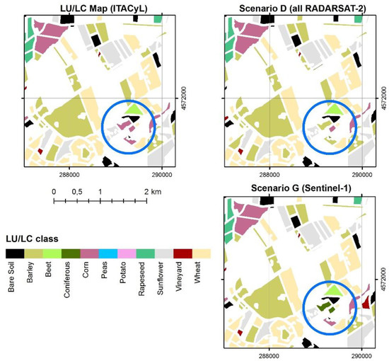
Figure 2.
Three subsets of the reference map (top, left) and the resulting maps after the classification of scenarios A and D (right). Some small differences are detected in the encircled area.
Table 6.
Overall accuracy and kappa coefficient.
Since the launch in April 2014 of Sentinel-1 by ESA, researchers have claimed the feasibility of dual-pol Sentinel-1 data as standalone input [53,54] or blended with optical data [55,56,57] for LU/LC classification. Bargiel [23] demonstrated a new crop classification approach that identified phenological sequence patterns of the crop types from a stack of Sentinel-1 data. He suggested the use of multitemporal SAR observables as a crucial factor for the improvement of crop classification.
The influence of the incidence angle for crop classification has also been explored. When the polarimetric observables derived from images at 36°, 31° and 25° were used by the classifier, the overall accuracies ranged from 83% to 86.6% and 0.79 to 0.84 for kappa coefficients (Table 6). The variation of the incidence angle seems not to influence the classification significantly in terms of overall accuracy, as it was observed that the highest accuracy of 86.6% (scenario A) was only slightly better (~3.5%) than the lowest accuracy (scenario C). In principle, shallower incidence angles are preferred for identification of crops [58] due to the importance of these angles to minimize backscatter contributions from the soil. However, there is no conclusive evidence in the literature about which angle or narrow range of angles are the most adequate for classification purposes. Therefore, the influence of incidence angle seems to be very low, opening the way to combine all available incidence angles (as in scenario D).
Regarding the training/validating sampling, as it was previously mentioned, a 60-40% criterion was used, that is, a random sampling containing 60% of the samples from the data were selected as training dataset and the remaining 40% as validating dataset. To test the dependence of the accuracy on the training/validating sample, a new classification of all scenarios was run using a new random sampling (preserving the 60-40% criterion). Table 7 shows the new results, where it is clear that the overall accuracy is quite similar to the results shown in Table 6. The highest differences in overall accuracy are shown for scenarios A (1.2%), B (0.9%) and C (0.8%), whereas for scenario D there was not any difference. Likewise, the differences for the kappa coefficient were negligible. Therefore, it can be concluded that, owing to the high number of samples, the accuracy does not vary depending on the sampling selection.
Table 7.
Random sampling: overall accuracy and kappa coefficient.
An important indicator of a successful classification is a high overall accuracy; however, getting an acceptable discrimination at the individual crop level is as important as a high overall accuracy, especially for some final applications. With this aim, the producer’s and user’s accuracies for individual covers are listed in Table 8.
Table 8.
Producer’s accuracies (PAs) and user’s accuracies (UAs) of individual cover types for RADARSAT-2 and Sentinel-1 data.
Results showed that rapeseed achieved the best PA results (>95%) in all scenarios, whereas barley achieved the second highest PA’s, ranging from 92.1% to 95.3%. The user’s accuracy (UA) of both crops was above 85% for all scenarios tested and achieved 100% for rapeseed in scenarios A and D. The results reported in this study for rapeseed agree with those found by Larrañaga and Álvarez-Mozos [35]. Cereals (i.e., wheat and barley) normally show a similar behaviour during the growing season due to their very similar plant structure and phenology, which causes difficulty in separating them based on their backscatter characteristics. However, the results showed that polarimetric SAR data at C-band were capable of classifying wheat and barley with high PAs ranging from 79.9% to 95.3%. Among these crops, barley achieved better results than wheat, with high PAs (95.1%, 95.1% and 95.3%) for scenarios A, E and D, respectively. In agreement with the result obtained in scenario D for barley, Larrañaga and Álvarez-Mozos [35] also reported a high PA for barley when different polarimetric observables were added to the H-V linear quad-pol data. The highest accuracy for wheat (88.3% and 88.1%) took place when Sentinel-1 dual-pol data (scenario G) or all polarimetric observables and images were used for classification (scenario D). In the specific confusion matrices for scenarios D (Figure 3a) and G (Figure 3b), most of the wheat plots were classified properly (356 out of 404 for scenario D and 364 out of 412 for scenario G). Only a small misclassification between wheat and barley was produced, which is explained by their similar plant structure. As shown in Table 8, RADARSAT-2 dual-pol scenario (F) showed good results (92.1% and 81.2%) for barley and wheat, respectively. The results reported from the dual-pol scenarios suggest that VH/VV dual polarization mode is a good choice for discriminating cereals from other crops and agrees with findings by McNairn et al. [8] and Veloso et al. [59]. Although barley and wheat were found to be well classified, the PA and UA of the third cereal considered, corn, are not as good as expected with regard to previous results found in the literature [39]. The best PA was shown in scenario G with Sentinel-1 dual-pol data (78.4%) and scenario E (78.2%). Corn in scenario C also provided the second poorest PA in this study, with just 54% of the corn plots classified correctly.
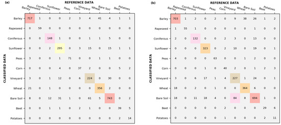
Figure 3.
Confusion matrices of classification for different scenarios: (a) Scenario D. (b) Scenario G.
The lowest accuracies were found for potatoes in 4 out of 7 scenarios, which were followed by corn. The scenario G is the worst of all scenarios, with a PA of 45.8%; this means that the classification at this scenario missed 54.2% of the potato areas on the ground, indicating a tendency for the model to misclassify potatoes. Due to their broad leaves, potatoes are mostly misclassified as beets (Figure 3b), which also have a similar plant structure. From all scenarios analysed for beet, scenario A (RADARSAT-2 at 36°) provided the highest PA (93.2%) followed by scenario E (83.7%). Scenario G (Sentinel-1 data using the backscattering coefficients and the ratio) also provided a high accuracy (82.9%) for beets. The accuracy reported in this study with Sentinel-1 data is higher than the accuracy provided by Sonobe et al. [56]. They achieved a PA of 74.6% using KELM (Kernel-based Extreme Learning Algorithm) and VV polarization data.
The PA of bare soil reached the highest accuracy (92.9%) in scenario D and accuracies above 84% for the rest of the scenarios. These good results for bare soil could be related to the use of cross-polarization as one of the inputs for the classifier. The use of cross-polarization makes the distinction between bare soil and vegetation-covered surfaces easier because the vegetation canopies depolarize the incident radiation more strongly than bare surfaces. Although bare soil provided a high PA in scenario D, 120 plots of bare soil were misclassified (Figure 3a); this shows, together with the vineyard, the highest confusion (61 plots, approximately 7% of the total of this category).
The potential of SAR images for classifying vineyards has also been investigated. Measurements on vineyards are not easy, given the high number of poles and metallic wires supporting the runners and the space between runners. As expected, no high accuracies were achieved for vineyards. Scenario A (RADARSAT-2 data at 36°) showed the highest PA (73.5%) and scenario C the lowest (61.3%). Scenario C was run using RADARSAT-2 data at 25°, so this poor accuracy could be related to the fact that at C-band, steep angles are more sensitive to ground conditions and less sensitive to the plant features; in contrast, shallower angles increase the interaction with the vegetation, therefore reducing the contribution of the soil and increasing the possibility of getting better accuracy, as it is shown for scenario A. Even though the poorer results are obtained for vineyard relative to other land covers, its accuracy could be considered acceptable.
The misclassification among forested areas, agricultural crops and grassland is expected in land-cover applications. However, L-band SAR data are known to provide an excellent source of information for forest cover mapping and it decreases the misclassification between covers due to its significant penetration capability relative to vegetation canopies. Our results showed high PAs and UAs, ranging from 83.1% to 91.5% and 82.5% to 94.9%, respectively. Scenario F (RADARSAT-2 dual-pol data) was found to provide the best PA that was slightly higher (0.5%) than scenario E (91%). Therefore, we could conclude that C-band SAR data were able to provide reliable classification of coniferous.
Sunflower and peas were also analysed. Sunflower obtained PAs above 81% in all scenarios with the exception of scenario C, which provided a PA of 74.2%. SAR data dual-pol scenarios (G and F) showed the highest accuracies (90% and 89.1%). The results found for sunflower using dual-pol data improved the results found by Skakun et al. [39]. However, Larrañaga and Álvarez-Mozos [35] obtained a PA of 100% for sunflower when they applied VV-VH dual-pol configuration of RADARSAT-2 data with just two backscattering coefficients in the two polarization channels. The difference in accuracy (~11%) between their results and our findings could be related to the fact that we added the ratio (VH/VV) as input into the classifier and because the number of sunflower plots and images is higher. Skakun et al. [39] used RADARSAT-2 backscattering intensity (VV, VH and HH) in beam mode (FQ8W) with incidence angle ranging from 26.1° to 29.4° to run a multitemporal crop classification in Ukraine. They found PA and UA of 60% and 63.5% for sunflower. Although the poorest accuracy (74.2%) found for sunflower was when RADARSAT-2 data at 25° were used in the classifier, our study demonstrated that the use of different polarimetric observables (beyond backscattering coefficients) improved the classification of sunflower when SAR data with low incidence angle are used in the classifier.
Finally, for peas, the highest PA was found in scenario D (95.9%), when all polarimetric observables and images were employed by the classifier. However, there is a high difference (19.2%) between the highest and the lowest accuracy (76.7%) provided by scenario C. In terms of UA, after rapeseed and coniferous, peas showed the highest accuracies (scenario A, 93.7%; scenario F, 95.9%). The results found for peas in this study improved those found by Larrañaga and Álvarez-Mozos [35]. Figure 3a shows that only three plots of peas were confused with barley and bare soil in this study.
In addition to the accuracy of the different combinations of SAR observables, the individual LU/LC analyses provided an interesting insight into the feasibility of the multitemporal series. After the results mentioned above, the best classification took place for rapeseed, barley, wheat and peas, all of which are spring crops, having their growing cycle between March and June, when the availability of images is higher (Table 3). Conversely, the worst results were found for summer crops, with growing cycles spanning until the beginning of fall (corn, potatoes and vineyard), which is not covered by the SAR series. Although with reasonably good results, sunflowers, beets and potatoes are also summer crops and could not achieve the optimal results found for the spring crops. Thus, it can be reasoned that, as suspected, the multitemporal-based classification clearly enhances the results of the polarimetric-based classification.
3.2. Attribute Evaluation
C5.0 shows the degree to which each attribute (SAR observable per date) contributes to the classifier and provides the percentage of training cases in the data file for which the value of that attribute is known and used for the construction of the classifier. Due to the large number of attributes used for each scenario, the attribute evaluation provided by C5.0 is very useful to know how individual attributes contribute to the construction of the classifier.
Figure 4 shows the attribute usage across the first three scenarios (A, B and C) that were run with 70, 60 and 60 attributes, respectively. In terms of polarimetric observables, the importance of the dominant alpha angle (α1) can be clearly seen, followed by the cross-polar backscattering coefficient (HV) and the backscattering ratios (HH/VV and HV/VV). The large usage of these polarimetric observables at specific acquisition dates implied that the information they supplied was useful for crop separation. Additionally, the contribution of the correlation between the co-polar channels (γHHVV) is important in scenario A. The least important polarimetric observables used in these scenarios were VV, γP1P2 and polarized difference phase (PPD).
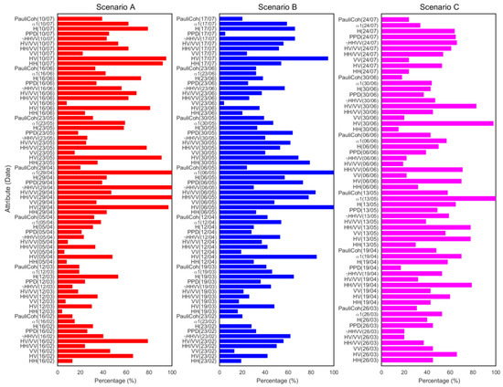
Figure 4.
Attribute contribution for scenarios A, B and C.
Scenario D (Figure 5) was the more complex scenario tested in this study with 200 attributes used. Like scenarios A, B and C, the dominant alpha angle (α1), γHHVV and the cross-polar backscattering coefficient (HV) are the most important observables. Many polarimetric observables at certain dates show null percentage, mainly because C5.0 does not show the attributes with values smaller than 1%.
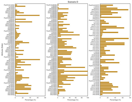
Figure 5.
Attribute contribution for scenario D.
The attributes of the last three scenarios (E, F and G) are shown in Figure 6. These scenarios used 56 (E), 42 (F) and 42 (G) attributes. Scenario E showed a clear influence of γHHVV on April 29, with 100% of the cases used in the classifier. In scenarios F and G (with just three polarimetric observables used), the cross-polar ratios (HV/VV and VH/VV) provided a high weight to the classifier.
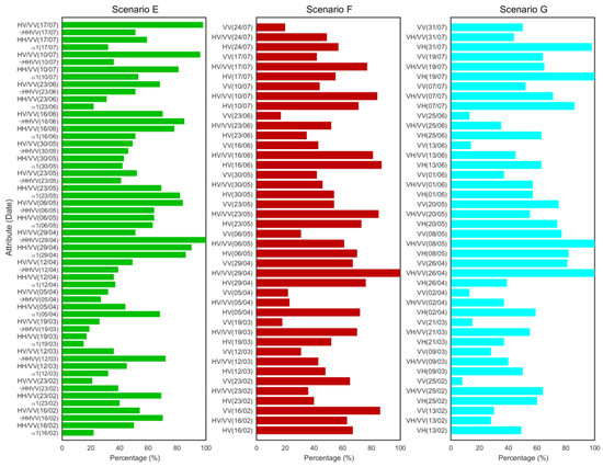
Figure 6.
Attribute contribution for scenarios E, F and G.
In terms of the acquisition dates, the RADARSAT-2 scenes with highest importance, along with the polarimetric observables, were April 29, May 06 and May 13. For Sentinel-1, the images were from April 26 and May 08. Skriver [60] reported a study to determine the optimum parameters for classification using airborne C- and L-band polarimetric SAR data. He found that at C-band, early acquisition, that is, in April, has a high discrimination potential but May acquisition provides the largest discrimination potential. He also reported that for May, the correlation coefficient between HH and VV as well as the ratio between HV and VV (among others) showed clear potential for separation. The results of this study agree with these findings. The fact that April and May had major relevance in the multi-temporal series is not surprising, since as previously mentioned, during this interval the most important vegetative growing stages of the crops in the area coincide, that is, maximum growth for the spring crops and development stage for the summer crops.
As a final test of the evaluation of attribute importance, a focussed pairwise crop analysis was conducted to estimate which observable contributed more to distinguishing wheat and barley, which were similar in structure and therefore expected to have a similar signal response. This test was performed for scenario D as a given example, which gathers all the possible attributes. The resulting pairwise analysis between these two crops (Figure 7) showed HH/VV as the highest contributor (100%) to separate both crops, followed by γHHVV.
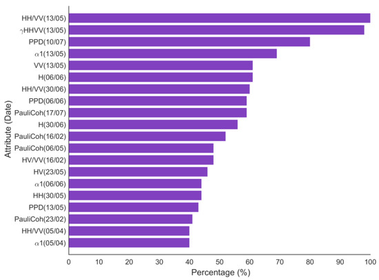
Figure 7.
Top 20 attributes used for the pairwise analysis.
Regarding the acquisition dates, the pairwise analysis with RADARSAT-2 emphasized the higher importance of May 13 as a key date reflecting the cereal growing cycle.
Feasible Applications Using the Importance of Attributes
The aim of the former analysis was to evaluate the weight of each observable in the classification to avoid redundant or useless data without losing accuracy. Choosing scenario D as an example, the feasibility of a reduced dataset for classification was tested. First, a new scenario (H) was created using the polarimetric observables with the three highest contributions in D: γHHVV, HV and α1 (Figure 5).
Comparing the classification results for D and H, a slight difference (0.7%) between scenario D (89.1%) and scenario H (88.4%) in terms of the overall accuracy was found. At individual crop level (Table 9), the use of attributes with the highest contribution improved the PA and UA accuracy of some crops compared with the results from scenario D (Table 9). For crops such as vineyard, beet and potato, the PA improvement between scenario D and H was of approximately 5% and corn showed the highest difference (8.3%). Other crops such as peas showed a slight decrease in PA from scenario H (88.2%) to scenario D (95.9%). All data considered, the accuracy of scenario H is similar to scenario D, whilst reducing dramatically the number of observables and therefore it is much more cost-effective.
Table 9.
Producer’s accuracies (PAs) and user’s accuracies (UAs) of individual cover types using only selected observables (scenario H) and the whole dataset (scenario D).
The second analysis consisted of a new classification only for the pairwise crops—wheat and barley—using solely the paramount observables resulting from the importance analysis of the previous section, that is, HH/VV and γHHVV (Scenario I). The accuracy assessment resulting for this new scenario (Table 10) is remarkable in comparison with the previous results of scenario D, in which all the observables were included. Both the PA and UA increased in I, meaning that the importance analysis afforded a powerful tool for separating crops with similar response, even improving the accuracy of the classification whilst reducing effectively the inputs needed (from 10 to 2, in this case).
Table 10.
Producer’s accuracies (PAs) and user’s accuracies (UAs) of barley and wheat using the whole dataset (scenario D), only selected observables (scenario I) and selected observables and dates (scenario J).
In order to explore the pairwise crop classification with limited inputs, a third analysis (named scenario J) was carried out from RADARSAT-2 data. This scenario was run using only the two main observables from Scenario I (HH/VV and γHHVV) and the three dates with highest importance (April 29, May 06 and May 13). Comparing the results of scenario J (Table 10) with the previous scenario I, it is noticeable that the accuracy has decreased but to a very small extent given the reduced dataset included on J. Indeed, if compared to the general scenarios A-G (with much more polarimetric observables and dates), the accuracy provided by scenario J is slightly higher (~0.5%) than scenarios B and F, whilst for wheat the PA is higher than for scenarios A, B, E and F. Again, the results of the importance analysis enabled a way to reduce the inputs whilst maintaining a remarkable accuracy.
4. Conclusions
The capability of polarimetric observables from multitemporal series of RADARSAT-2 and Sentinel-1 images for crop-type classification was assessed, together with an analysis of the influence of the incidence angle and the importance of the observables. A dataset of more than 3000 plots of 11 crop types and land covers was used as a reference map to obtain the confusion matrices and therefore to validate all the combinations of the 10 SAR observables proposed.
The use of all polarimetric RADARSAT-2 observables and scenes available produced clear benefits in terms of the overall accuracy (scenario D), which was approximately 90%. However, other alternatives tested with RADARSAT-2, such as those that use incidence angles separately (scenarios A, B and C) also afforded very high overall accuracies. Since these latter alternatives require less data, they may be considered more cost-effective than the extensive dataset required in D. Thus, it may be concluded that even with the limited revisit time of 24 days of RADARSAT-2, the strength of the multitemporal series using polarimetric data reinforced its high capability to classify land covers. Nonetheless, the joint use of only dual-pol Sentinel-1 and RADARSAT-2 also provided very good accuracies greater than 85%. The results from the kappa coefficient confirmed all these results.
When the incidence angle was considered separately (cases A, B and C aforementioned), the variation between cases in terms of overall accuracy and kappa is only 3.5% and 6%, respectively. After the results, the incidence angle seems not to influence neither the classification broadly nor the individual results for each cover, which were heterogeneous and not conclusive.
Regarding the individual results for each specific land cover, the rapeseed crop obtained the best accuracy for all scenarios—higher than 95%. The good separation of spring cereals, typically difficult owing to their similar structure and phenology, was also remarkable. The addition of polarimetric SAR data at C-band allowed classifying wheat and barley with high very high PAs and UAs. In contrast, vineyard, corn and potatoes showed the worst results, followed by sunflowers, beets and peas. The middling results for those summer crops may be explained by their shorter time coverage of images during summer-early fall, highlighting the importance of a complete multitemporal coverage for the whole growing season, as in the case of wheat and barley.
The contribution of each SAR observable per date to the different alternatives of classification was also analysed by means of the attribute study available in the C5.0 algorithm. Among the polarimetric observables, the dominant alpha angle (α1) showed a predominant contribution with RADARSAT-2 at all the different incidence angle alternatives, whereas for the dual polarization scenario of Sentinel-1 (G), the cross-polar channel VH and the VH/VV ratio were the most important. Those findings about the performance of each observable would help in future classifications by reducing the use of redundant and potentially misleading data. Following this thread, it has been proven that a classification using only the key observables improved on, or afforded similar accuracy to, the previous classifications with the whole dataset, whilst dramatically reducing the number of data and the computing time. This finding applied not only for a classification of all the categories in a whole but also for discriminating crop pairs with low separability, for example, wheat versus barley. The analysis of importance was also useful for defining which dates were crucial in the classification. The results showed that May acquisitions were the key dates in the classification, coinciding with the maximum growing period of many crops in the area. When the crops have a summer cycle, the separation worsened.
Finally, although the polarimetric capabilities of RADARSAT-2 and Sentinel-1 are rather different, the multitemporal approach reinforced the classification process and provided similar satisfactory results for the different scenarios of classification. Additional features that could also help to improve the accuracy of the classification of individual crop types are interferometric parameters, such as coherence, as well as textural information within the intensity values. In addition, further tests should be conducted over other different climatic and environmental conditions to expand and consolidate the method.
Author Contributions
All authors contributed significantly to this manuscript. R.V.-D. conceived the research and performed the analysis. R.V.-D. and B.A.-P. processed the satellite data. J.M.L.-S. and N.S. provided constructive suggestions. Finally, R.V.-D. prepared the manuscript draft and the rest of the authors contributed to the final manuscript and approved it.
Funding
RADARSAT-2 Data and Products @ MacDonald, Dettwiler and Associates Ltd. (MDA, 2015)—All Rights Reserved RADARSAT is an official trademark of the Canadian Space Agency (CSA). All RADARSAT-2 images have been provided by MDA and CSA in the framework of the SOAR-EU2 Project ref. 16375. This study was supported by the Spanish Ministry of Science, Innovation and Universities, State Research Agency (AEI) and the European Regional Development Fund under projects TEC2017-85244-C2-1-P, ESP2015-67549-C3-3 and ESP2017-89463-C3-3-R.
Conflicts of Interest
The authors declare no conflict of interest.
References
- Kogan, F.; Kussul, N.; Adamenko, T.; Skakun, S.; Kravchenko, O.; Kryvobok, O.; Shelestov, A.; Kolotii, A.; Kussul, O.; Lavrenyuk, A. Winter wheat yield forecasting in Ukraine based on Earth observation, meteorologicaldata and biophysical models. Int. J. Appl. Earth Obs. Geoinf. 2013, 23, 192–203. [Google Scholar] [CrossRef]
- Gallego, F.J.; Kussul, N.; Skakun, S.; Kravchenko, O.; Shelestov, A.; Kussul, O. Efficiency assessment of using satellite data for crop area estimation in Ukraine. Int. J. Appl. Earth Obs. Geoinf. 2014, 29, 22–30. [Google Scholar] [CrossRef]
- Becker-Reshef, I.; Justice, C.; Sullivan, M.; Vermote, E.; Tucker, C.; Anyamba, A.; Small, J.; Pak, E.; Masuoka, E.; Schmaltz, J.; et al. Monitoring Global Croplands with Coarse Resolution Earth Observations: The Global Agriculture Monitoring (GLAM) Project. Remote Sens. 2010, 2, 1589–1609. [Google Scholar] [CrossRef]
- McNairn, H.; Ellis, J.; Van Der Sanden, J.J.; Hirose, T.; Brown, R.J. Providing crop information using RADARSAT-1 and satellite optical imagery. Int. J. Remote Sens. 2002, 23, 851–870. [Google Scholar] [CrossRef]
- Ban, Y. Synergy of multitemporal ERS-1 SAR and Landsat TM data for classification of agricultural crops. Can. J. Remote Sens. 2003, 29, 518–526. [Google Scholar] [CrossRef]
- Blaes, X.; Vanhalle, L.; Defourny, P. Efficiency of crop identification based on optical and SAR image time series. Remote Sens. Environ. 2005, 96, 352–365. [Google Scholar] [CrossRef]
- Brisco, B.; Brown, R.J. Multidate SAR/TM synergism for crop classification in western Canada. Photogramm. Eng. Remote Sens. 1995, 61, 1009–1014. [Google Scholar]
- McNairn, H.; Champagne, C.; Shang, J.; Holmstrom, D.; Reichert, G. Integration of optical and Synthetic Aperture Radar (SAR) imagery for delivering operational annual crop inventories. ISPRS J. Photogramm. Remote Sens. 2009, 64, 434–449. [Google Scholar] [CrossRef]
- Schotten, C.G.J.; Van Rooy, W.W.L.; Janssen, L.L.F. Assessment of the capabilities of multi-temporal ERS-1 SAR data to discriminate between agricultural crops. Int. J. Remote Sens. 1995, 16, 2619–2637. [Google Scholar] [CrossRef]
- Torres, R.; Snoeij, P.; Geudtner, D.; Bibby, D.; Davidson, M.; Attema, E.; Potin, P.; Rommen, B.; Floury, N.; Brown, M.; et al. GMES Sentinel-1 mission. Remote Sens. Environ. 2012, 120, 9–24. [Google Scholar] [CrossRef]
- Aschbacher, J.; Milagro-Pérez, M.P. The European Earth monitoring (GMES) programme: Status and perspectives. Remote Sens. Environ. 2012, 120, 3–8. [Google Scholar] [CrossRef]
- Chen, K.S.; Huang, W.P.; Tsay, D.H.; Amar, F. Classification of multifrequency polarimetric SAR imagery using a dynamic learning neural network. IEEE Trans. Geosci. Remote Sens. 1996, 34, 814–820. [Google Scholar] [CrossRef]
- Ferrazzoli, P.; Guerriero, L.; Schiavon, G. Experimental and model investigation on radar classification capability. IEEE Trans. Geosci. Remote Sens. 1999, 37, 960–968. [Google Scholar] [CrossRef]
- Ferrazzoli, P.; Paloscia, S.; Pampaloni, P.; Schiavon, G.; Sigismondi, S.; Solimini, D. The potential of multifrequency polarimetric SAR in assessing agricultural and arboreous biomass. IEEE Trans. Geosci. Remote Sens. 1997, 35, 5–17. [Google Scholar] [CrossRef]
- Bouman, B.A.M.; Uenk, D. Crop classification possibilities with radar in ERS-1 and JERS-1 configuration. Remote Sens. Environ. 1992, 40, 1–13. [Google Scholar] [CrossRef]
- Dobson, M.C.; Pierce, L.E.; Ulaby, F.T. Knowledge-based land-cover classification using ERS-1/JERS-1 SAR composites. IEEE Trans. Geosci. Remote Sens. 1996, 34, 83–99. [Google Scholar] [CrossRef]
- McNairn, H.; Shang, J.; Jiao, X.; Champagne, C. The contribution of ALOS PALSAR multipolarization and polarimetric data to crop classification. IEEE Trans. Geosci. Remote Sens. 2009, 47, 3981–3992. [Google Scholar] [CrossRef]
- Schmugge, T.J.; Kustas, W.P.; Ritchie, J.C.; Jackson, T.J.; Rango, A. Remote sensing in hydrology. Adv. Water Resour. 2002, 25, 1367–1385. [Google Scholar] [CrossRef]
- Skriver, H.; Svendsen, M.T.; Thomsen, A.G. Multitemporal C- and L-band polarimetric signatures of crops. IEEE Trans. Geosci. Remote Sens. 1999, 37, 2413–2429. [Google Scholar] [CrossRef]
- Larrañaga, A.; Álvarez-Mozos, J.; Albizua, L.; Peters, J. Backscattering Behavior of Rain-Fed Crops Along the Growing Season. IEEE Geosci. Remote Sens. Lett. 2013, 10, 386–390. [Google Scholar] [CrossRef]
- Skriver, H. Crop Classification by Multitemporal C- and L-Band Single- and Dual-Polarization and Fully Polarimetric SAR. IEEE Trans. Geosci. Remote Sens. 2012, 50, 2138–2149. [Google Scholar] [CrossRef]
- Skriver, H.; Mattia, F.; Satalino, G.; Balenzano, A.; Pauwels, V.R.N.; Verhoest, N.E.C.; Davidson, M. Crop Classification Using Short-Revisit Multitemporal SAR Data. IEEE J. Sel. Top. Appl. Earth Obs. Remote Sens. 2011, 4, 423–431. [Google Scholar] [CrossRef]
- Bargiel, D. A new method for crop classification combining time series of radar images and crop phenology information. Remote Sens. Environ. 2017, 198, 369–383. [Google Scholar] [CrossRef]
- Hariharan, S.; Mandal, D.; Tirodkar, S.; Kumar, V.; Bhattacharya, A.; Lopez-Sanchez, J.M. A Novel Phenology Based Feature Subset Selection Technique Using Random Forest for Multitemporal PolSAR Crop Classification. IEEE J. Sel. Top. Appl. Earth Obs. Remote Sens. 2018, 11, 4244–4258. [Google Scholar] [CrossRef]
- Kussul, N.; Lemoine, G.; Gallego, J.; Skakun, S.; Lavreniuk, M. Parcel based classification for agricultural mapping and monitoring using multi-temporal satellite image sequences. In Proceedings of the International Geoscience and Remote Sensing Symposium (IGARSS), Milan, Italy, 26–31 July 2015; pp. 165–168. [Google Scholar]
- Mandal, D.; Kumar, V.; Bhattacharya, A.; Rao, Y.S.; Siqueira, P.; Bera, S. Sen4Rice: A processing chain for differentiating early and late transplanted rice using time-series sentinel-1 SAR data with google earth engine. IEEE Geosci. Remote Sens. Lett. 2018, 15, 1947–1951. [Google Scholar] [CrossRef]
- Siachalou, S.; Mallinis, G.; Tsakiri-Strati, M. A Hidden Markov Models Approach for Crop Classification: Linking Crop Phenology to Time Series of Multi-Sensor Remote Sensing Data. Remote Sens. 2015, 7, 3633–3650. [Google Scholar] [CrossRef]
- Canisius, F.; Shang, J.; Liu, J.; Huang, X.; Ma, B.; Jiao, X.; Geng, X.; Kovacs, J.M.; Walters, D. Tracking crop phenological development using multi-temporal polarimetric Radarsat-2 data. Remote Sens. Environ. 2017, 210, 508–518. [Google Scholar] [CrossRef]
- Mascolo, L.; Lopez-Sanchez, J.M.; Vicente-Guijalba, F.; Nunziata, F.; Migliaccio, M.; Mazzarella, G. A Complete Procedure for Crop Phenology Estimation with PolSAR Data Based on the Complex Wishart Classifier. IEEE Trans. Geosci. Remote Sens. 2016, 54, 6505–6515. [Google Scholar] [CrossRef]
- Brisco, B.; Brown, R.J.; Gairns, J.G.; Snider, B. Temporal Ground-Based Scatterometer Observations of Crops in Western Canada. Can. J. Remote Sens. 1992, 18, 14–21. [Google Scholar] [CrossRef]
- Foody, G.M.; McCulloch, M.B.; Yates, W.B. Crop classification from C-band polarimetric radar data. Int. J. Remote Sens. 1994, 15, 2871–2885. [Google Scholar] [CrossRef]
- Lee, J.-S.; Grunes, M.R.; Pottier, E. Quantitative comparison of classification capability: Fully polarimetric versus dual and single-polarization SAR. IEEE Trans. Geosci. Remote Sens. 2001, 39, 2343–2351. [Google Scholar]
- Loosvelt, L.; Peters, J.; Skriver, H.; De Baets, B.; Verhoest, N.E.C. Impact of Reducing Polarimetric SAR Input on the Uncertainty of Crop Classifications Based on the Random Forests Algorithm. IEEE Trans. Geosci. Remote Sens. 2012, 50, 4185–4200. [Google Scholar] [CrossRef]
- Deschamps, B.; McNairn, H.; Shang, J.; Jiao, X. Towards operational radar-only crop type classification: Comparison of a traditional decision tree with a random forest classifier. Can. J. Remote Sens. 2012, 38, 60–68. [Google Scholar] [CrossRef]
- Larrañaga, A.; Álvarez-Mozos, J. On the added value of quad-pol data in a multi-temporal crop classification framework based on RADARSAT-2 imagery. Remote Sens. 2016, 8, 335. [Google Scholar] [CrossRef]
- Sonobe, R.; Tani, H.; Wang, X.; Kobayashi, N.; Shimamura, H. Random forest classification of crop type using multi-temporal TerraSAR-X dual-polarimetric data. Remote Sens. Lett. 2014, 5, 157–164. [Google Scholar] [CrossRef]
- McNairn, H.; Kross, A.; Lapen, D.; Caves, R.; Shang, J. Early season monitoring of corn and soybeans with TerraSAR-X and RADARSAT-2. Int. J. Appl. Earth Obs. Geoinf. 2014, 28, 252–259. [Google Scholar] [CrossRef]
- Zhang, Y.; Zhang, J.; Zhang, X.; Wu, H.; Guo, M. Land Cover Classification from Polarimetric SAR Data Based on Image Segmentation and Decision Trees. Can. J. Remote Sens. 2015, 41, 40–50. [Google Scholar] [CrossRef]
- Skakun, S.; Kussul, N.; Shelestov, A.Y.; Lavreniuk, M.; Kussul, O. Efficiency Assessment of Multitemporal C-Band Radarsat-2 Intensity and Landsat-8 Surface Reflectance Satellite Imagery for Crop Classification in Ukraine. IEEE J. Sel. Top. Appl. Earth Obs. Remote Sens. 2016, 9, 3712–3719. [Google Scholar] [CrossRef]
- Sonobe, R.; Tani, H.; Wang, X.; Kobayashi, N.; Shimamura, H. Discrimination of crop types with TerraSAR-X-derived information. Phys. Chem. Earth 2015, 83–84, 2–13. [Google Scholar] [CrossRef]
- Zeyada, H.H.; Ezz, M.M.; Nasr, A.H.; Shokr, M.; Harb, H.M. Evaluation of the discrimination capability of full polarimetric SAR data for crop classification. Int. J. Remote Sens. 2016, 37, 2585–2603. [Google Scholar] [CrossRef]
- Valcarce-Diñeiro, R.; Lopez-Sanchez, J.M.; Sánchez, N.; Arias-Pérez, B.; Martínez-Fernández, J. Influence of Incidence Angle in the Correlation of C-band Polarimetric Parameters with Biophysical Variables of Rain-fed Crops. Can. J. Remote Sens. 2018, 44, 643–659. [Google Scholar] [CrossRef]
- Nafría, D.A.; del Blanco, V.; Bengoa, J.L. Castile and Leon Crops and Natural Land Map. In Proceedings of the WorldCover Conference, Frascati, Rome, Italy, 14–16 March 2017. [Google Scholar]
- Cloude, S.R.; Pottier, E. A review of target decomposition theorems in radar polarimetry. IEEE Trans. Geosci. Remote Sens. 1996, 34, 498–518. [Google Scholar] [CrossRef]
- Schubert, A.; Small, D.; Miranda, N.; Geudtner, D.; Meier, E. Sentinel-1A Product Geolocation Accuracy: Commissioning Phase Results. Remote Sens. 2015, 7, 9431–9449. [Google Scholar] [CrossRef]
- Quinlan, J.R. C4.5: Programs for Machine Learning; Morgan Kaufmann Publishers, Inc.: San Mateo, CA, USA, 1992. [Google Scholar]
- Champagne, C.; McNairn, H.; Daneshfar, B.; Shang, J. A bootstrap method for assessing classification accuracy and confidence for agricultural land use mapping in Canada. Int. J. Appl. Earth Obs. Geoinf. 2014, 29, 44–52. [Google Scholar] [CrossRef]
- Powers, R.P.; Hay, G.J.; Chen, G. How wetland type and area differ through scale: A GEOBIA case study in Alberta’s Boreal Plains. Remote Sens. Environ. 2012, 117, 135–145. [Google Scholar] [CrossRef]
- Freund, Y.; Schapire, R.E. Experiments with a New Boosting Algorithm. In Machine Learning: Proceedings of the Thirteenth International Conference; Bari, Italy, 1996; Morgan Kaufmann Publishers Inc.: San Francisco, CA, USA, 1996; pp. 148–156. [Google Scholar]
- Congalton, R.G. A review of assessing the accuracy of classifications of remotely sensed data. Remote Sens. Environ. 1991, 37, 35–46. [Google Scholar] [CrossRef]
- Story, M.; Congalton, R.G. Accuracy assessment: A user’s perspective. Photogramm. Eng. Remote Sens. 1986, 52, 397–399. [Google Scholar]
- Cohen, J. A Coefficient of Agreement for Nominal Scales. Educ. Psychol. Meas. 1960, 20, 37–46. [Google Scholar] [CrossRef]
- Balzter, H.; Cole, B.; Thiel, C.; Schmullius, C. Mapping CORINE Land Cover from Sentinel-1A SAR and SRTM Digital Elevation Model Data using Random Forests. Remote Sens. 2015, 7, 14876–14898. [Google Scholar] [CrossRef]
- Son, N.T.; Chen, C.F.; Chen, C.R.; Minh, V.Q. Assessment of Sentinel-1A data for rice crop classification using random forests and support vector machines. Geocarto Int. 2018, 33, 587–601. [Google Scholar] [CrossRef]
- Kussul, N.; Lemoine, G.; Gallego, F.J.; Skakun, S.V.; Lavreniuk, M.; Shelestov, A.Y. Parcel-Based Crop Classification in Ukraine Using Landsat-8 Data and Sentinel-1A Data. IEEE J. Sel. Top. Appl. Earth Obs. Remote Sens. 2016, 9, 2500–2508. [Google Scholar] [CrossRef]
- Sonobe, R.; Yamaya, Y.; Tani, H.; Wang, X.; Kobayashi, N.; Mochizuki, K.I. Assessing the suitability of data from Sentinel-1A and 2A for crop classification. GISci. Remote Sens. 2017, 54, 918–938. [Google Scholar] [CrossRef]
- Zhou, T.; Pan, J.; Zhang, P.; Wei, S.; Han, T. Mapping winter wheat with multi-temporal SAR and optical images in an urban agricultural region. Sensors 2017, 17, 1210. [Google Scholar] [CrossRef] [PubMed]
- Rosenthal, W.D.; Blanchard, B.J. Active microwave responses: An aid in improved crop classification. Photogramm. Eng. Remote Sens. 1984, 50, 461–468. [Google Scholar]
- Veloso, A.; Mermoz, S.; Bouvet, A.; Le Toan, T.; Planells, M.; Dejoux, J.F.; Ceschia, E. Understanding the temporal behavior of crops using Sentinel-1 and Sentinel-2-like data for agricultural applications. Remote Sens. Environ. 2017, 199, 415–426. [Google Scholar] [CrossRef]
- Skriver, H. Signatures of polarimetric parameters and their implications on land cover classification. In Proceedings of the International Geoscience and Remote Sensing Symposium (IGARSS), Barcelona, Spain, 23–27 July 2007; pp. 4195–4198. [Google Scholar]
© 2019 by the authors. Licensee MDPI, Basel, Switzerland. This article is an open access article distributed under the terms and conditions of the Creative Commons Attribution (CC BY) license (http://creativecommons.org/licenses/by/4.0/).