Abstract
The Three Gorges Reservoir (TGR) in China, with the largest dam in the world, stores a large volume of water and may influence the Earth’s gravity field on sub-seasonal to interannual timescales. Significant changes of the total water storage (TWS) might be detectable by satellite-based data provided by the Gravity Recovery and Climate Experiment (GRACE) mission. To detect these store water changes, effects of other factors are to be removed first from these data due to band-limited representation of near-surface mass changes from GRACE. Here, we evaluated three current popular land surface models (LSMs) basing on in situ measurements and found that the WaterGAP Global Hydrology Model (WGHM) demonstrates higher correlation than other analyzed models with the in-situ rainfall measurement. Then we used the WGHM outputs to remove climate-induced TWS changes, such as surface water storage, soil, canopy, snow, and groundwater storage. The residual results (GRACE minus WGHM) indicated a strong trend (3.85 ± 2 km3/yr) that is significantly higher than the TGR analysis and hindcast experiments (2.29 ± 1 km3/yr) based on in-situ water level measurements. We also estimated the seepage response to the TGR filling, contributions from other anthropogenic dams, and used in-situ gravity and GPS observations to evaluate dominant factors responsible for the GRACE-based overestimate of the TGR volume change. We found that the modeled seepage variability through coarse-grained materials explained most of the difference between the GRACE based estimate of TGR volume changes and in situ measurements, but the agreement with in-situ gravity observations is considerably lower. In contrast, the leakage contribution from 13 adjacent reservoirs explained ~74% of the TGR volume change derived from GRACE and WGHM. Our results demonstrate that GRACE-based overestimate TGR mass change mainly from the contribution of surrounding artificial reservoirs and underestimated TWS variations in WGHM simulations due to the large uncertainty of WGHM in groundwater component. In additional, this study also indicates that reservoir or lake volume changes can be reliably derived from GRACE data when they are used in combination with relevant complementary observations.
1. Introduction
Since its launch in 2002, the Gravity Recovery and Climate Experiment (GRACE) mission has been proven to be a unique tool to monitor total water storage (TWS) variability at large spatial scales (>300 km) by measuring changes in the Earth’s gravity field. GRACE provides valuable information for studying the phenomena that reflect changes due to the climate and human activity, e.g., regional water mass variability, droughts, and floods [1], ice sheet mass balance in Antarctica and Greenland [2], water balance in Asia’s high mountains [3], as well as the groundwater storage decrease in Northern India [4], the North China Plain [5], and in the US High Plains and Central Valley [6]. Generally, the limited spatial resolution of the GRACE data (~100,000 km2) is a benefit when estimating changes in TWS at large regional to global scales. The most commonly used GRACE products are monthly gravity field changes with a maximum resolution up to 60 degree/order of the Stokes coefficients. The higher degrees are significantly suppressed and biased by potential errors, which requires extensive post-processing to reduce the noise and signal loss. For these purposes, destriping and filtering methods have been developed with the aim to improve final products [7,8].
Truncation and filtering of GRACE data reduces the signal amplitude and significantly reduces the spatial resolution. Furthermore, GRACE observations reflect a sum of many effects e.g., climate-induced water storage changes including: surface water storage, soil, canopy, snow, and groundwater storage, and human-induced the impoundment of reservoirs and groundwater pumping, those hydrological components are difficult to separate without a-priori information from the effect of TWS changes [9]. For this purpose, most previous studies used land surface models (LSMs) or hydrological models to remove these effects from GRACE [10,11]. For example, LSMs was used to estimate the contributions of TWS compartments (e.g., soil, snow and surface water storage) to GRACE-based results, for the purpose of quantifying depletion rates of aquifer systems like groundwater changes [4,5,6]. However, global LSMs and hydrological estimates of surface water storage (rivers and lakes) are characterized by high uncertainties, especially for artificial reservoirs behind dams, which are usually not included in most LSMs. Consequently, these uncertainties bias final GRACE estimates.
Several studies employed GRACE products to estimate TWS changes in small areas, which, in principle, cannot be resolved by GRACE, such as rivers, lakes, flooded areas, small aquifer systems, and other localized regions [12]. This type of water redistribution, which could be quite large in total, is often related to human activities, socio-economic, and climate changes and geological disasters. In previous studies, such small-scale phenomena have been studied with special methods depending on signal source characteristics. Several of these approaches employed corrections to restore the signal loss due to filtering, e.g., the additive method [13], the multiplicative method [14], the scaling factor method [10], and the data-driven method [15]. However, these methods still depend on model assumptions and size of the study area. Another approach implies using a-priori information on water level changes, such as in-situ measurements and radar altimetry, to remove their effects. With this approach, Longuevergne et al. [12] estimated large reservoir and lake storage components by combining the satellite radar altimetry and GRACE data. Using GRACE data, satellite altimetry, and in-situ observations, seasonal variability and trends in water storage and lake level were examined in the great lakes’ region in East Africa and Tibetan Plateau [16,17,18,19].
The China’s Three Gorges Reservoir (TGR) is one of the largest reservoirs used for hydropower generation in the world. The Three Gorges Dam (TGD) is a gravity dam that spans the Yangtze River near the town of Sandouping, Yichang, in Hubei Province (Figure 1). The total capacity of the TGR is 39.3 km3. When the TGR is full, the water level reaches 175 m above sea level, which is 110 m higher than the level of the river. This man-made lake has on average a length of about 660 km and a width of 1.12 km with a total surface equal to 1084 km2. Although the TGR width is much smaller than the spatial resolution of GRACE observations, the enormous total water volume exceeds the sensitivity threshold for GRACE data [20]. Wang et al. [21] estimated TGR monthly volume changes based on GRACE data and the WaterGAP Global Hydrology Model (WGHM) and compared the residual signal (GRACE minus WGHM) with in-situ measurements from April 2002 and May 2010. Their results indicated that GRACE can retrieve the true amplitudes of large surface water storage changes in a concentrated TGR area, and overestimate of GRACE-WGHM mass anomalies might come from a variety of contributing factors, e.g., uncertainties of WGHM (i.e., WGHM may underestimate soil moisture, water ponds, and snow), groundwater recharge (seepage) during filled TGR and the influence of neighboring reservoirs or lakes, but they did not quantitatively evaluate those influencing factors. Compared to satellite observations, surface gravity and deformation (GPS) measurements are more sensitive to water storage changes in the TGR and their variations can be modeled using a water load model derived from the Digital Elevation Model (DEM) data [22].
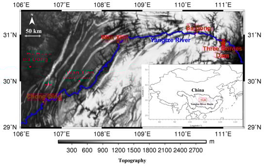
Figure 1.
Topography and location of the Three Gorges Reservoir (TGR) study area. At maximum water level (175 m), the TGR stretches approximately 600 km along the Yangtze River (blue curve) from the TGD (red star) to Chongqing.
Since the TGR extends along the thin Yangtze River, the impact of other hydrological factors is significant. Our goal is to improve the GRACE estimates by combining them with in-situ measurements and water mass distribution data. In this study, we first evaluated the sensitivity of GRACE data to the TGR water storage changes. Then, we selected three popular LSMs to quantitatively evaluate their simulations basing on in-situ measurements. We also examined the effects of uncertainties in GRACE observations and other factors related to the surrounding hydrological signal, such as underground reservoirs in aquifers (leakage and groundwater recharge). Furthermore, we determined whether the influence of surrounding reservoirs could be quantitatively assessed using additional information about other contributions to regional volume changes observed by GRACE.
2. Data Sources
2.1. GRACE
We selected spherical harmonic datasets from February 2003 to December 2012 (114 months), from the GRACE Release 05 (RL05), which contains monthly gravity field solutions generated by the Center for Space Research (CSR) at the University of Texas. Each monthly GRACE field consists of a set of Stokes coefficients (Clm and Slm) up to 60 degree and order (l and m). The original GRACE C20 coefficients were replaced with results inferred from the satellite laser ranging [23], while for the degree-one coefficient the solution from Swenson et al. [24] has been used. The Stokes coefficients from A et al. [25] were used to remove effects from Glacial Isostatic Adjustment (GIA), which are small in the TGR region. The monthly solutions had been filtered using a Gaussian smoothing operator with an averaging radius of 350 km in order to suppress errors at high degrees [26].
2.2. Land Surface Models
As was mentioned above, GRACE provides vertically integrated mass variations hampering a simple process separation. In other words, the GRACE data are influenced by many factors and it is impossible to use them alone to separate from the effects of the surface water storage and water stored in the reservoir, as well as of the soil moisture and groundwater [27]. The primary purpose of this study was to estimate changes in TGR’s surface water storage from GRACE-based TWS. Thus, it needs us first to remove effects due to other water storage components, what has been done by applying output from LSM simulations. Unfortunately, the impact of LSM uncertainties is significant, especially in regions that are highly irrigated and/or arid and semiarid regions. Moreover, different LSMs provide diverse estimates for these signals. Here, we tested three LSMs to select the optimal hydrological model: (i) The Noah, VIC, and Mosaic version of GLDAS-1 (Global Land Data Assimilation System) with a spatial resolution of 1° × 1° quantify variability in soil moisture storage [28]; (ii) the WGHM model with the same resolution provides the continental water cycle including water storage compartments at a spatial resolution of 0.5° × 0.5°, such as soil moisture within the effective root zone of vegetated areas, groundwater canopy water, snow, and surface water in rivers, lakes, reservoirs, and wetlands (not including artificial lakes) [29]; and (ii) version 4.5 of the Community Land Model (CLM4.5), which includes terrestrial hydrological processes such as soil moisture, snow, canopy, river storage, and groundwater at a spatial resolution of 1° × 1° [30].
2.3. In-Situ Measurements
In situ measurements of stored water in the TGR offer an opportunity to evaluate the surface dynamic response due to temporal variability in water storage. In this study we used the Shuttle Radar Topography Mission (SRTM) DEM data combined with in-situ water level measurements to construct a TGR stored water model. The linear vertical relative height error of SRTM is less than 10 m for 90% of data [31]. The SRTM DEM data covers the Earth between 60°N and 57°S at resolution levels of 3 arc-seconds (or 90 m), which can be used to analyze the TGR’s static storage capacity, e.g., the volume, length, and water coverage area at different surface water levels [32,33]. In the latest version of SRTM DEM V4.1 data, the gaps and missing data issues have been resolved by applying a gap-filling interpolation algorithm. The errors of total static volumes derived from SRTM DEM data are in the range 0.1–0.3 km3 [21].
These DEM data were used to delineate the reservoir and surrounding regions (Figure 2). Water level data of TGR were obtained from the China Three Gorges Corporation database over the period of 2003~2012. Furthermore, we used six years of absolute gravity determinations (A10) at three locations (yellow dots in Figure 2) near the TGD (red star in Figure 2). The A10 observations were mainly collected during the lowest (June) and highest (December) water level periods. Relative gravity measurements (gPhone) were conducted for about 5 months at the station located 38 km from the dam (white triangle in Figure 2 and used to detect surface gravity effects during the water level rise from 145 m to 175 m in 2011. We also used vertical displacements obtained between July 2010 and March 2013 from one permanent GPS station in the TGR (pink triangle in Figure 2), which belongs to the Continental Tectonic Environmental Monitoring Network of China. Detailed information on the in-situ A10, gPhone, and GPS measurements and the data processing method can be found in Wang et al. [22].
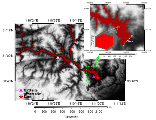
Figure 2.
Water volume distribution (a portion of the loading model near the dam) used for numerical simulation. The effective water surface is determined by the difference between bed elevation and the water level (i.e., 175 m). The locations of in-situ A10, gPhone, and GPS measurements are shown as yellow dots, white triangle, and pink triangle, respectively.
In this study, we collected the monthly precipitation data (rainfall amount) in Yangtze River Basin (YRB) during the period of 2003–2012 from China Meteorological Data Sharing Service System (CMDSSS) of the China meteorological administration. Rainfall data consist of a national gridded time series with a 0.5° × 0.5° spatial resolution that covers the time span from 1961 to 2013. The gridded average monthly rainfall of YRB shown in Figure 6a. In addition, we calculated the time series of monthly in-situ rainfall basing on more than 300 stations (locations shown in Figure 6a) refer to the YRB monthly average. We estimated the time series of monthly in-situ soil moisture storage (SMS, locations shown in Figure 6a) using the equation SMS = n × D × dSM/dt, n is soil porosity; D is soil depth, i.e., multiple soil moisture layers (0–15, 15–25, and 25–75 cm); dSM/dt is soil relative saturation. We first calculated the time series of SMS in the corresponding layer and added them together, and then subtracted the multi-year average SMS to obtain the time series of 0–75 cm SMS anomaly in the study area. Moreover, monthly groundwater level measurements from 136 wells in our study region (Figure 6a) were used to calculate the area-weighed equivalent groundwater storage. A constant specific yield of 0.03 according to an average value from 19 sites (most stations do not provide this value), was used to convert the groundwater level to groundwater storage.
3. Numerical Simulation of the Response to Three Gorges Reservoir Filling
Basing on a gridded loading model and the power law relationship between volume (V, km3) and water level (H, m) (V = 0.2968 × 1.0284H, Wang et al. [21]), we performed the following simulations: (1) water contributions from the TGR and other reservoirs at the GRACE spatial resolution scale; (2) horizontal flow during water filling in the TGR; (3) gravity field and displacement effects at in-situ gravimeters and GPS locations (A10, gPhone, and GPS sites in Figure 2) caused by water load and estimated leakage.
The simulation (1) to model the TGR signal from GRACE data was performed in two steps: (i) we computed the Stokes coefficients corresponding to a 1 km3 increase of the TGR volume on a 0.0008335-degree grid (~90 m × 90 m) over TGR. The grid spans the entire length of the reservoir. The same height (H) was assigned to each point, which value corresponds to a total volume increase of 1 km3. We calculated a set of Stokes coefficients for each point, and then summed the coefficients for all points. The resulting set of Stokes coefficients up to degree and order 60 represented a 1 km3 increase of the TGR volume; (ii) we used the Stokes coefficients from (i) to estimate time-dependent coefficients for TGR using the water level time series from in-situ measurements. Water level was converted to volume using the equation V = 0.2968 × 1.0284H (Figure 3). Finally, we calculated the TGR Stokes coefficient variability with time (T) as a product of the Stokes coefficients multiplied by the volume V (T).
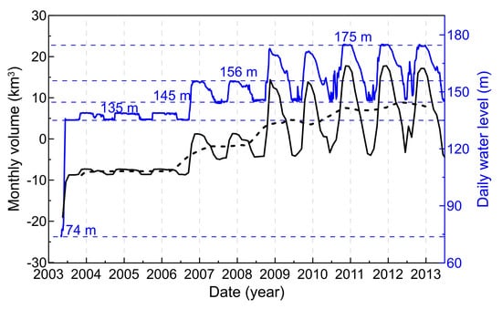
Figure 3.
In-situ daily water level (blue solid curve) and monthly volume after removed mean volume (black solid curve) in the TGR from 2003 to 2012. The blue dashed lines represent four stages of the TGR filling: prefilling (74 m) and the first (135 m), second (156 m), and third stages (175 m). The black dashed curve is the smoothed TGR prediction.
In simulation (2) we modeled the total water leakage around TGR as a function of time, using the equation for horizontal flow in an unconfined aquifer: (i.e., horizontal water flow from a reservoir in Figure 4a), applying the approach of Wang and Anderson [34]. Here, h(x,t) is the top of the saturated zone (x is the distance of horizontal seepage), K is the hydraulic conductivity, S is the specific yield, which refers to the drainable or fillable porosity, and h is the elevation of the upper boundary of the water table. The equation is solved for h(x,t) in an unconfined aquifer with the boundary condition h(0,t) = h0(t) and with a no flow condition (dh/dx = 0) on the right hand side. It is clear that the solution depends not only on the hydraulic conductivity and fillable porosity, but also on the width of leakage (the x-axis shown in Figure 4a). Additionally, it depends on the choice of the initial value for h(x). The hydraulic conductivity, also known as permeability, is the ability of rocks or unconsolidated material to transmit water. Although the hydraulic conductivity is partly controlled by intergranular porosity, it is important to note that very fine-grained rocks and materials with disconnected pores tend to have low conductivity.
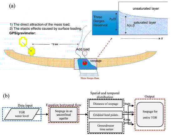
Figure 4.
(a) Diagram showing horizontal flow and response in terms of gravity and deformations during the TGR water filling. (b) Flowchart for the leakage estimation using horizontal flow modeling for the entire TGR.
The percentage of water in rocks that promptly drains out is known as the specific yield. Fine-grained materials, such as clay or shale, are likely to have a specific yield of 5% or less, even if the porosity is about 20 to 30%. Coarse-grained materials, such as coarse sandstone, can have specific yields that are closer to their actual porosity in the range 20 to 35%. In this study, we used the mean value for the hydraulic conductivity and specific yield according to Freeze and Cherry [35], K = 7 × 10⁻⁷ m/s, S = 0.02 (seepage-1) and K = 7 × 10⁻⁶ m/s, S = 0.17 (seepage-2) for fine-grained and coarse-grained rocks, respectively. To compute the water seepage volume, we constructed a dense grid of points surrounding TGR within 2.5 km of the shoreline. We calculated the distance from each point to the TGR and interpolated the solution h(x,t) for that grid point at every time step to estimate the temporal change in the top of the saturated zone. The integration over the whole area then gives the total mass balance at each time step (Figure 4b).
In simulation (3), we combined the TGR water storage model (DEM and water level) with the leakage results from simulation (2) to model gravity effects and surface deformations. The gravitational effects caused by TGR mass changes can be separated into two factors: (1) the direct gravitational attraction of water and (2) secondary effects caused by the Earth’s deformation in response to changes in surface load. We modeled direct attraction by dividing the reservoir into a large number of thin vertical water columns (Figure 2) and integrating the effects of all columns. Then we modeled the elastic effects related to the Earth’s deformation by surface loads using Green’s functions [36] based on the PREM reference Earth model with the continental crust [37]. The effect of viscosity on gravity and displacement changes has been neglected, because it is much smaller than the elastic ones over the short time period considered here [20].
4. Results
4.1. GRACE Estimated Mass Changes and Sensitivity Kernels
Figure 5a shows the TWS change across TGR on a 0.5° × 0.5° grid, which combines the trends for each GRACE Stokes coefficient over the entire 10-year time span (2003–2012). A positive trend was identified over the TGR and surrounding region, including the middle and lower plains and the Yangtze River. Although TGR is located close to the centre of the mass increase derived from GRACE, the reason for this increase as well as its significance is unclear. The GRACE-based TWS change may be also affected by soil moisture, groundwater and surface water storage. Additionally, hydropower reservoirs that were constructed after 2000 may also have contributed to the observed volume increase, such as the Danjiangkou Dam northeast of TGR.
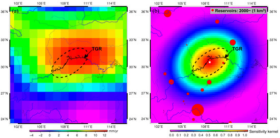
Figure 5.
(a) Trends in TWS changes in the TGR and surrounding areas derived from the Center for Space Research (CSR) GRACE product (RL05) after Gaussian filtering (350 km) from 2003–2012 in mm/yr. (b) GRACE averaging kernels used to estimate the TGR mass variability. Red circles show 13 large reservoirs surrounding TGR since 2000; their sizes represent different reservoir capacities.
To calculate GRACE time series for TGR and compare them with the simulation (1), we constructed an averaging kernel using the convolution method described by Swenson and Wahr [38]. We used the TGR “basin function” that was derived from 175-m grid points and DEM data. The averaging kernel technique based on a weighted Gaussian convolution was used to construct monthly time-series from GRACE Stokes coefficients [39]. Figure 5b shows the sensitivity kernel, which is relatively uniform within the study area but spans over a long distance from TGR. Therefore, the resulting time-series after applying the averaging kernel also include contributions outside TGR from other reservoirs (red circles in Figure 5b). To recover unbiased mass estimates for this region, the scaling factor method was used to restore the filtered TWS time-series. The method suggested by Wahr et al. [39] requires construction of a set of simulated Stokes coefficients, which represents the signal from a uniformly distributed 1 cm (10−5 km) water depth change over the TGR. This gives water volumes of 10−5 km × area change of 1084 km2 for TGR (0.01084 km3). We apply our GRACE analysis procedure to these simulated Stokes coefficients, to infer equivalent water height (EWH, unit cm) for TGR. Based on the simulated scaling factor (k) = 1 (cm)/EWH (cm), monthly GRACE estimates of water thickness (10−5 km) were multiplied by scaling factor to obtain variations in the total mass per area of the TGR, and then multiplied by area change of 1084 km2 for TGR resulting in GRACE-based water mass change (km3).
4.2. Assessing Land Surface Models
We selected the YRB as study area (Figure 3) to assess LSMs primarily because TGR is located in the middle of the river’s main channel, while previous studies have indicated that most LSM products have relatively large uncertainties in rivers and lakes [11,12]. Two other important factors, which could differ across diverse LSMs, are large seasonal rainfall cycling, when the average monthly rainfall reaches about 100 mm (Figure 6a), and climate- and human-induced terrestrial water resource changes in YRB.
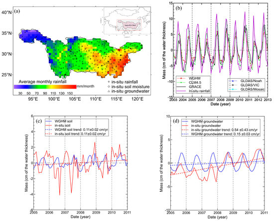
Figure 6.
(a) Average monthly rainfall (in mm/month) in China based on in-situ observations for 2003–2012 from the CMDSSS. (b) Changes in the Yangtze River Basin (YRB) water storage (units: cm) from GRACE, GLDAS (Noah, VIC and Mosaic), WaterGAP Global Hydrology Model (WGHM), and version 4.5 of the Community Land Model (CLM4.5) models after Gaussian smoothing and applying the averaging kernel, and the time series of monthly in-situ rainfall (after removed mean value refer to YRB) from China Meteorological Data Sharing Service System (CMDSSS) for the selected area. (c) Times series of monthly in-situ observation of soil moisture (units: cm) from 122 sites located in YRB and soil moisture from WGHM outputs from 2005 to 2010. (d) Times series of monthly in-situ observation of groundwater (units: cm) from 136 sites located in YRB and groundwater from WGHM outputs from 2005 to 2010. (c,d) both removed mean value refer to the YRB, cm/yr represents cm per year, in-situ observation of soil moisture data also provided by CMDSSS and in-situ observation of groundwater data (available only from 2005 to 2010) are obtained from the groundwater level yearbook compiled by the Institute of China Geological Environment Monitoring [41].
In Figure 6b the different LSM model simulations with GLDAS (Noah, VIC and Mosaic), WGHM, and CLM4.5 are compared, where the same processing approach has been applied as for the GRACE data (i.e., the Gaussian smoothing function and averaging kernel method). The phases of all model simulations agree with the GRACE results, while the TWS changes from both GRACE and LSMs indicate that YRB is mainly controlled by climate changes. For example, more rainfall over YRB in summer expanded terrestrial water reserves, while two severe drought events that occurred in 2006 and 2011 resulted in the reduction of TWS (Figure 6b). The seasonal amplitude of all three GLDAS simulations is also much smaller than for WGHM and CLM4.5 because the GLDAS model does not include anthropogenic and climate-driven surface water storage and groundwater changes [28]. The CLM4.5 simulations have even larger seasonal amplitudes than GRACE-derived TWS and WGHM results, especially in summer. The difference between CLM4.5 and WGHM is likely due to the differences in forcing precipitation datasets, e.g., WGHM is forced by a combination of the Global Precipitation Climatology Centre monthly precipitation data sets from 1901 to present, which are calculated from global stations on a 1.0° × 1.0° grid [40], while the CLM4.5 simulations are forced by precipitation inputs on a 2.5° × 2.5° grid from the Global Precipitation Climatology Project, which are bias-corrected using merged satellite-gauge precipitation values.
To quantitatively evaluate which LSM better fits to YRB and to separate the TGR signal from the GRACE solutions, the relative correlation coefficients of TWS variability between in-situ measurements and LSMs were calculated (Table 1). The correlation coefficients for in-situ measurements and WGHM is 0.85, which is higher than the results for other LSMs or even GRACE. This indicates that WGHM and GRACE are more consistent with the in-situ measurements in the YRB. We also used the Nash–Sutcliffe efficiency (NSE) [42] to calculate a degree of statistical similarity between in-situ measurements and GRACE and LSMs. The NSE is the normalized statistical parameter that indicates how well the observed and simulated data fit a 1:1 linear relationship [43]. In this case, the NSE coefficient was used to examine the correspondence between in-situ rainfall and GRACE- or LSMs-based TWS changes. For all of the LSMs, the correspondence reflected in NSE values between the in-situ data and WGHM (NSE: 0.64) is higher than that of in-situ data and other LSMs (CLM4.5: 0.52; GLDAS/Noah: 0.35). Furthermore, the TWS annual variability and the secular trends from LSMs and estimated from GRACE were compared (Table 1). The GRACE-derived increased linear rate 0.37 cm/yr for YRB because they are affected by all hydrological components, including artificial reservoirs. However, the CLM4.5 output also has a continuous increase (0.14 cm/yr) in water storage and relative larger annual amplitude (5.18 cm) than other models for the region. In particular, the amplitude of CLM4.5 is larger than the GRACE data, implying that the CLM4.5 results with the river component likely include some of the signal from TGR or another reservoir. Consequently, we adopted WGHM as the primary model for removing climate-induced TWS effects, in order to study only anthropogenic effects. This choice is consistent with previous studies [21].

Table 1.
The total water storage correlation and Nash–Sutclffe efficiency (NSE) of in-situ measurements, GRACE, and the land surface models (LSMs).
We should clarify that WGHM (almost other LSMs) is a conceptual water balance model with grossly simplified process representations [44]. The forcing data of WGHM is calibrated only by tuning a runoff generation parameter against observed river discharge [45], so hydrological component variations in WGHM may also differ from in-situ measurements (e.g., WGHM may underestimate ‘ground truth’ of TWS changes in TGR area assess by Wang et al. [21]). Here, we used in-situ observation of soil moisture and groundwater versus WGHM outputs to verify the difference between the two modes in the YRB. Figure 6c shows in-situ observation of soil moisture has a large seasonal fluctuation relative to WGHM-based soil moisture and both show a small and consistent long-term linear trend (0.11 cm/yr) in the YRB. But the long-term trend of WGHM-based groundwater (0.15 cm/yr) is lower than the in-situ measured results (0.54 cm/yr), which means that the model simulation does not reflect the true groundwater recharge due to abundant rainfall and less water withdrawals for irrigation in the YRB [11].
4.3. Time Series of the GRACE-Based Three Gorges Reservoir Volume
Time series of GRACE-derived volume change after removing the WGHM output (Figure 7) can be directly related to human-induced water storage changes (i.e., TGR) within the sensitivity kernel range (Figure 5b). The GRACE minus WGHM changes (dashed orange line) demonstrate that short-term fluctuations superimpose a long-term trend. The short-term fluctuations are mainly due to measurement errors related to the system-noise in the K-Band range-rate observations, accelerometer errors and orbit uncertainties, spatial and temporal sampling errors, and inaccuracies in the background models (e.g., the aliasing errors, which are clearly expressed as north–south oriented strips in the gravity field). The dashed black curve shows the effects of three TGR filling stages. The water level first increased from ~70 m to 135 m in June 2003 and then reached 156 m in October 2006. After 2008, the water level reached ~175 m, which was the highest water level, changing in strong seasonal cycles under manual control.
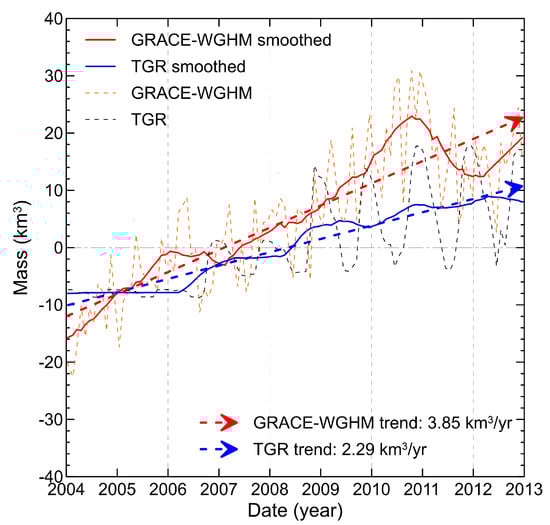
Figure 7.
Volume changes estimated for the GRACE-minus-WGHM model (dashed orange curve for the original and solid red curve for the smoothed results) and the TGR prediction based on in-situ measurements (dashed black curve for the original and solid blue curve for the smoothed results).
With respect to long-term variability, the smoothed results indicated that the GRACE estimates after WGHM removal show an increase of the TGR volume (solid red line), which is consistent with Wang et al. [21] and with the TGR predictions from in-situ measurements (solid blue line). However, the smoothed residual signal (GRACE − WGHM) demonstrates much larger increase relative to the TGR predictions: 3.85 ± 2 km3/yr versus 2.29 ± 1 km3/yr respectively. The errors represent uncertainties in the fit, while real uncertainties mainly depend on errors in the WGHM data, leakage of the signal from outside, and GRACE measurement errors. In fact, the errors of LSM outputs are difficult to assess due to uncertainties in the synthesized data [11]. Compared to the other LSMs analyzed here, WGHM shows highest agreement with in-situ measurements in the YRB. We also found that WGHM has no clear trend in the entire YRB but this result is likely to underestimate the true long-term trend of groundwater (Figure 6d). Because of the current groundwater well sites in the TGR and surrounding areas (i.e., GRACE averaging kernels shown in Figure 5b) are very sparse, it is difficult to obtain accurate groundwater changes. Assuming that the rate of groundwater change in the sensitive area of GRACE is the same as the entire YRB, the underestimation of groundwater due to WGHM uncertainty is likely one of the contributors to the linear trend of the GRACE minus WGHM estimates. In addition, the different between GRACE-based and in-situ observed mass changes could be due to errors in GRACE data or, more likely, due to external or internal leakage effects. The GRACE observations might also be affected by other signal sources, which not only represent contributions from adjacent areas but also reservoir leakage or groundwater recharge during TGR filling.
4.4. Reservoir Leakage Due to Three Gorges Reservoir Filling
Based on simulation (2) (Section 3) we estimated the total seepage around TGR using two different permeability coefficients (i.e., seepage-1 and seepage-2 shown in Figure 8a). Volume variability from GRACE has a larger trend than what could be explained by the TGR alone (Figure 7). Modeling volume variability caused by seepage-2 through coarse-grained rocks can lead to good agreement; for instance, the 3.85 ± 2 km3/yr trend from the GRACE results is in good agreement with the TGR water volume estimates that include seepage (i.e., TGR’s 2.29 ± 1 km3/yr + seepage-2′s 1.03 km3/yr). However, the seepage contribution is small for fine-grained rocks (i.e., seepage-1), for which the trend 0.12 km3/yr (Figure 8a) is too small to explain the GRACE data. In fact, it is unrealistic to model the entire TGR shoreline with two simple and uniform seepage coefficients. Due to its length of nearly 600 km, it is difficult to determine detailed and realistic physical infiltration conditions. For example, most of the TGR shoreline is rocky along the main corridor of the Yangtze River, but some soil or coarse-grained rocks might be typical in some branches of the Yangtze River. We inferred that the actual horizontal flow should be between these two alternative scenarios (seepage-1 and seepage-2), when the vertical seepage is neglected in consequence of an already saturated river bottom.
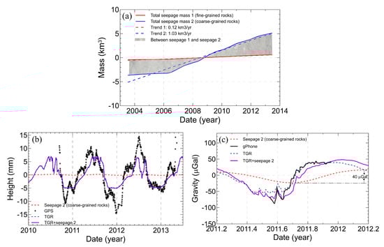
Figure 8.
(a) Simulations of the total seepage volume surrounding TGR using two permeability coefficients: K = 7 × 10⁻⁷ m/s, S = 0.02 (seepage-1, red curve) and K = 7 × 10⁻⁶ m/s, S = 0.17 (seepage-2, blue) for fine-grained and coarse-grained rocks, respectively. (b) Time series of displacements from GPS measurements and model predictions (dashed blue curve represents TGR alone and solid purple curve represents TGR with seepage-2 in 2010–2013. (c) Similar to (b), but for gravity effects.
Predictions of surface displacements and gravity field from simulation (3) suggest that GPS (Figure 8b) and gPhone (Figure 8c) data are in good agreement with TGR predictions without including seepage during filling the reservoir. On the other hand, including gravity effects of the seepage-2 model made the agreement worse for the gPhone data. Using the fine-grained rock parameter in the seepage model did not improve the agreement with gPhone data, but the model could no longer explain the GRACE results. The effects of seepage on GPS vertical displacements are also unimportant.
5. Discussion
5.1. Effects of Small-Scale Mass Change on GRACE Estimates
This study showed that the large concentrated volume changes in TGR are detectable by GRACE, when these observations are combined with LSMs. In general, errors in GRACE surface mass estimates over a fixed area can be separated into two categories: errors in the Stokes coefficients after post-processing (Gaussian smoothing, regional averaging, and scaling the estimated masses), and those caused by effects of other signal sources, such as leakage and correction error, etc. Stokes coefficients of the GRACE solution are truncated to a limited degree lmax (e.g., lmax = 60 for the CSR solutions). Therefore, the spatial resolution of GRACE products is limited to ~330 km (region-A in Figure 9a). Consequently, the truncated to lmax solution is sensitive to mass changes well outside the region of interest (e.g., lakes and reservoirs like region-B in Figure 9a). Many applications using GRACE data require estimates of mass variability for specific regions, e.g., changes in the Greenland or Antarctic ice sheets, or in river basins’ water storage. These problems can be better addressed by constructing specific averaging functions optimized for those regions. In general, more accurate results can be obtained for larger regions. In this study, mass changes were estimated by creating specific averaging functions covering the TGR. The averaging kernel method employs Gaussian smoothing at each point and integrates them over the whole area. In this case, the averaging kernel technique is also limited due to the spatial resolution of GRACE, and the averaging function extends several hundred kilometers outside the region (Figure 5b).
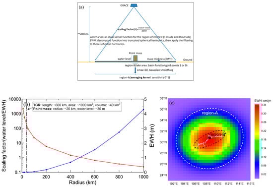
Figure 9.
(a) Schematic diagram showing usage of the averaging function to restore realistic mass changes in GRACE results. (b) EWH scaling factor changes for different smoothing radii. (c) Trends in the TGR prediction after truncation to degree 60 and application of a 350 km Gaussian filter. The dashed white circle shows region-A and the black dot shows region-B.
Figure 9a shows the gravitational attraction of a fixed mass at the GRACE level. To recover unbiased estimates for this region, we have to scale the estimated mass signals and to restore the original amplitude. Assuming a uniform distribution of masses within the region of interest (e.g., a uniform 1 cm water change over region-B), k can be defined as the scaling factor (k) = (water level)/EWH based on an ideal kernel function for the study region (1 inside and 0 outside). The effect of this mass was converted into truncated spherical harmonics and then smoothed with the 350 km Gaussian filter. After that, the rest of the signal within the region was considered as the scaling factor. Figure 9b shows the scaling factors and EWH changes for disks of different size, where the radius varied from 10 km to 1000 km with a uniform 1 cm water layer. Our tests showed that the EWH values (blue curve in Figure 9b) increased as the size of the disc became larger, which resulted in the scaling factors (k) = 1/EWH dropping from hundreds or even thousands to less than 1 (red curve in Figure 9b). For example, if the TGR area was concentrated in one disk with a 20 km radius, it would lead to a larger scale factor (k = 583). Ideally, i.e., without leakage outside the basin, application of the above method assumes that monthly GRACE estimates of water thicknesses should be multiplied by the scaling factors (k) = 1/EWH to obtain variations of total water thickness in region-B with corresponding changes of volume. Figure 9c shows modeling results for long-term TGR changes at the GRACE resolution scale. We found that the most obvious increase in EWH is concentrated in region-B but is still significant for several hundred kilometers outside. This suggests that in order to use GRACE to monitor mass changes in TGR (region-B in Figure 9c), it is necessary to extend the study area (region-A in Figure 9c) and to consider more hydrological information in that extended area.
5.2. Short- and Long-Term Surface Gravity Changes
Here, we describe the use of in situ measurements from gravimeters (gPhone and A10) near TGR to detect gravity field variations caused by water level changes. Gravitational effects were separated into the direct gravitational attraction of the water and secondary effects caused by the Earth’s crustal deformation in response to changes in surface load. The modeled results described by Wang et al. [22] showed that gravity along the edge of the lake can vary seasonally by up to a few hundred micro-gals if the gravimeter is situated well above the lake surface. The predicted variations caused by the ~1-m fluctuations of the lake level can be on the order of a few to 10 micro-gals.
We compared the model predictions with the data from five years of repeated absolute gravity (A10) campaigns at several locations, as well as five months of continuous relative gravity (gPhone) measurements at a single site near TGR. For short-term or seasonal variability, gPhone observations at a single location show very good agreement with the modeled results without seepage, but there was not enough data to assess an agreement in case of the seepage effects under coarse-grained rocks’ conditions (Figure 8c). For this, we used gravity residuals from gPhone observations after removing model predictions to verify if there exists continuous seepage around the observation point due to the TGR filling. Differences between observed and predicted signals could indicate the TWS variability due to rainfall (i.e., blue shadow in Figure 10a). However, it is worth noting that the magnitude of the predicted results is slightly larger than the observed data during the low water level in summer. This difference is due to some systematic errors in the simulated results. For instance, the numerical computations employed the water load model, which was developed for a static inundated area below the 175 m water level. These results are higher than the gPhone observations obtained at the ~145 m water level.
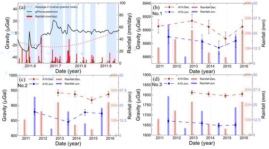
Figure 10.
(a) Gravity residuals from gPhone observations, corrected for predicted leakage effects due to TGR filling. (b–d) A10 absolute gravity measurements at two levels (145 m and 175 m) for 3 stations in the network (Figure 2); the error bars of A10 represent total measurement uncertainty at ~10 micro-gals (μGal) levels. Lower plots in (a–d) show daily and monthly rainfall changes at the Zigui weather station.
For long-term or inter-annual variability, five periods between 2010 and 2015 were observed at the A10 sites near TGD (Figure 4). The A10 data were divided into two groups according to the observation periods in June with the lowest water level (~145 m) and in December with the highest water level (~175 m). The gravity changes are plotted at these three stations in Figure 10b–d. It is clear that strongest gravity changes reaching several hundred micro-gals occurred in the regions near the reservoir shoreline between June and December. We found that there was no significant linear trend in the A10 results, which implies that there was no long-term continuous leakage in the area surrounding the A10 sites. According to the changes in the monthly rainfall rate in June and December (red and blue steps), the TWS change caused by the inter-annual rainfall oscillations were the main factor influencing the long-term gravity variability. Therefore, annual fluctuations in the A10 data reflected the hydrological mass anomalies due to changes in the climate but not due to the long-term seepage during TGR filling. Furthermore, we observe a good correlation between the surface water storage changes from the China Water Resources Bulletins published by the Ministry of Water Resources with major drought events in YRB in 2013–2014 [46]. Locally, those mass anomalies could cause changes of 10–20 micro-gals in the gravity signal.
5.3. Contributions of Other Anthropogenic Reservoirs to the GRACE Signal
Since 2000, the number of large reservoirs and water storage capacity in YRB has substantially increased. We used the reservoir capacity data from the International Commission on Large Dams (ICOLD) to calculate the water storage change in 13 large reservoirs surrounding TGR (Table 2). The selection of those large reservoirs was mainly based on their capacity (>0.5 km3), which is equivalent to an increase of 10 m in the water level of a disc-type reservoir with a radius of 4 km, or a river-type reservoir with a width of 1 km and a length of 50 km. Furthermore, the averaging kernel (Figure 5b) was not constant in the TGR area: the kernel weight for the TGR, Jiangkou, Pengshui, and Shuibuya reservoirs was equal to 1, while the weights for the Yinzidu, Danjiangkou, and Zipingpu reservoirs were set to 0.6, 0.5, and 0.2, respectively.
Table 2.
Detailed information of the water storage for the analyzed reservoirs (except TGR) within the GRACE sensitivity kernel.
To estimate contributions from these 13 reservoirs to GRACE-based results, we used the same simulation (1) method described above. Opposed to TGR, we only used a single disk to describe each reservoir (red discs in Figure 5b). They were summed up to obtain combined, time-dependent Stokes coefficients for the reservoirs. Because water level data for other reservoirs are currently not available to the public, a special technique was applied to reproduce them. We used the total volume (Final_Volume) and the completion date (T_end) of each reservoir assuming that the reservoir began filling at time T_(start) and that it was filled uniformly from the initial volume to the final volume at time T_end. According to Table 2 the total storage capacity change during 2003~2013 for all 13 reservoirs was 12.78 km3 after scaling by the kernel weights. Our statistical results showed that the contribution from the large reservoirs around TGR is equivalent to ~33% of its total capacity (39.3 km3) and cannot be ignored. If we distribute this amount uniformly over the 10-year study period (2003~2013), it would produce an increasing linear trend of about 1.16 km3/yr. This result is close to the difference between GRACE derived and TGR trends (1.56 km3/yr). Therefore, the volume change of the 13 largest reservoirs can explain ~74% of the GRACE-WGHM-TGR estimated mass changes. Note that we did not fully calculate the contribution of other reservoirs with a capacity of less than 0.5 km3. If these small reservoirs were taken into account, the results would likely fit the GRACE data better. Thus, our analysis suggests that the GRACE-based overestimation of the TGR volume changes reflects the effects of surrounding reservoirs.
6. Conclusions
The controlled TGR experiment provided a unique opportunity to evaluate time-variable gravity measurements from GRACE with a limited spatial resolution in combination with complementary data. This study demonstrates that TWS variations in relatively small reservoirs can be monitored by GRACE in combination with LSMs, remote sensing and in-situ measurements, which are used to separate various TWS components. We conclude that:
1. Our findings indicated that the WGHM demonstrates (with correlation coefficient of 0.85 and NSE = 0.64) better correlation than other analyzed models (GLDAS and CLM4.5) with the time series of monthly in-situ rainfall refer to the YRB’s monthly average. The rate of volume increase from GRACE-WGHM predictions was 3.85 ± 2 km3/yr from 2003 to 2012, which is larger than the result derived from in situ estimates for TGR (2.29 ± 1 km3/yr). The comparison results show that the partial hydrological component (e.g., soil and groundwater) from WGHM outputs is a worse agreement with the in-situ measurements in the YRB. The WGHM simulation might underestimated TWS variations due to the large uncertainty of WGHM in groundwater component. Therefore, more in-situ groundwater data should be collected in the TGR and surrounding areas in next step for provide more accurate corrections to GRACE results.
2. Our study showed that the GRACE-based overestimate might be explained by the modeled seepage variability through the coarse-grained materials, but the agreement with in-situ gPhone gravity observations and TGR predictions was much worse in this case. Furthermore, the long-term in-situ A10 absolute gravity observations also suggest that the overestimation of the GRACE-based TGR volume change is likely not a result of the seepage from the reservoir.
3. The sensitivity kernels suggested that the GRACE estimates are substantially affected by signals from outside the TGR region. We quantitatively evaluated the contributions from the adjacent reservoirs and concluded that the residual signal (GRACE − WGHM − TGR) is close to the sum of the volume change due to surrounding reservoirs. Therefore, the difference between GRACE-based results and TGR in-situ measurements is likely due to the volume changes in the neighboring reservoirs.
Finally, this study not only explore the novel routine for monitoring the mass changes and its environmental response in the water cycle, but also it is help for investigating the impacts of human activities on water resources. Basing on multi-source data we can effectively minimize the effects resulting from uncertainties of satellite observations, e.g., improve estimation accuracy of GRACE Follow-On mission, which is successfully launched in May 2018.
Author Contributions
Conceptualization, L.W.; Methodology, L.W. and X.M.; Validation, M.K.K., M.T., C.C. and X.M.; Writing—original draft, L.W.; Writing—review and editing, L.W., M.K.K., M.T. and C.C.
Funding
This work is supported by the National Natural Science Foundation of China (41874090, 41504065, 41574070 and 41604060) and the Fundamental Research Funds for the Central Universities, China University of Geosciences (Wuhan).
Acknowledgments
We thank two anonymous reviewers for their insightful comments, which help to an improvement of this manuscript. We gratefully thank the data distribution agencies who provided the publicly released data used in this study. The GRACE solutions used in this study are available from CSR (ftp://podaac.jpl.nasa.gov/allData/grace/L2/CSR/RL05/). The DEM data are obtained from the Shuttle Radar Topography Mission version 4.1 (http://srtm.csi.cgiar.org) and the water level data of the TGR are obtained from the database of the China Three Gorges Corporation (http://www.ctg.com.cn). The precipitation products were downloaded from CMDSSS (http://data.cma.cn/data/cdcindex.html). The GLDAS model data is provided by the NASA Goddard Earth Sciences Data and Information Services Center (http://disc.sci.gsfc.nasa.gov/). We are thankful to Andreas Güntner for providing the WGHM model outputs. We are grateful to John Wahr for providing CLM4.5 Stokes coefficients produced by National Center for Atmospheric Research (NCAR). The 13 large reservoir capacity data are available from the International Commission on Large Dams (http://www.icold-cigb.net/). GPS were downloaded from China Earthquake Data Center (http://www.eqdsc.com).
Conflicts of Interest
The authors declare no conflict of interest.
References
- Reager, J.T.; Thomas, B.F.; Famiglietti, J.S. River basin flood potential inferred using GRACE gravity observations at several months lead time. Nat. Geosci. 2014, 7, 588–592. [Google Scholar] [CrossRef]
- Velicogna, I.; Sutterley, T.C.; van den Broeke, M.R. Regional acceleration in ice mass loss from Greenland and Antarctica using GRACE time-variable gravity data. J. Geophys. Res. Space Phys. 2014, 41, 8130–8137. [Google Scholar] [CrossRef]
- Yi, S.; Sun, W. Evaluation of glacier changes in high-mountain Asia based on 10 year GRACE RL05 models. J. Geophys. Res. 2014, 119, 2504–2517. [Google Scholar] [CrossRef]
- Rodell, M.; Velicogna, I.; Famiglietti, J.S. Satellite-based estimates of groundwater depletion in India. Nature 2009, 460, 999–1002. [Google Scholar] [CrossRef] [PubMed]
- Feng, W.; Zhong, M.; Lemoine, J.M.; Biancale, R.; Hsu, H.T.; Xia, J. Evaluation of groundwater depletion in North China using the Gravity Recovery and Climate Experiment (GRACE) data and ground-based measurements. Water Resour. Res. 2013, 49, 2110–2118. [Google Scholar] [CrossRef]
- Scanlon, B.R.; Longuevergne, L.; Long, D. Ground referencing GRACE satellite estimates of groundwater storage changes in the California Central Valley, USA. Water Resour. Res. 2012, 48, W04520. [Google Scholar] [CrossRef]
- Swenson, S.; Wahr, J. Post-processing removal of correlated errors in GRACE data. Geophys. Res. Lett. 2006, 33, L08402. [Google Scholar] [CrossRef]
- Zhang, Z.Z.; Chao, B.F.; Lu, Y.; Hsu, H.T. An effective filtering for GRACE time-variable gravity: Fan filter. Geophys. Res. Lett. 2009, 36, L17311. [Google Scholar] [CrossRef]
- Song, C.; Ke, L.; Huang, B.; Richards, K.S. Can mountain glacier melting explains the grace-observed mass loss in the southeast Tibetan plateau: From a climate perspective? Glob. Planet. Chang. 2015, 124, 1–9. [Google Scholar] [CrossRef]
- Landerer, F.; Swenson, S. Accuracy of scaled GRACE terrestrial water storage estimates. Water Resour. Res. 2012, 48, W04531. [Google Scholar] [CrossRef]
- Long, D.; Longuevergne, L.; Scanlon, B.R. Global analysis of approaches for deriving total water storage changes from GRACE satellites. Water Resour. Res. 2015, 51, 2574–2594. [Google Scholar] [CrossRef]
- Longuevergne, L.; Wilson, C.R.; Scanlon, B.R.; Cretaux, J.F. GRACE water storage estimates for the Middle East and other regions with significant reservoir and lake storage. Hydrol. Earth Syst. Sci. 2013, 17, 4817–4830. [Google Scholar] [CrossRef]
- Klees, R.; Zapreeva, E.A.; Winsemius, H.C.; Savenije, H.H.G. The bias in GRACE estimates of continental water storage variations. Hydrol. Earth Syst. Sci. 2007, 11, 1227–1241. [Google Scholar] [CrossRef]
- Longuevergne, L.; Scanlon, B.R.; Wilson, C.R. GRACE Hydrological estimates for small basins: Evaluating processing approaches on the High Plains Aquifer, USA. Water Resour. Res. 2010, 46, W11517. [Google Scholar] [CrossRef]
- Vishwakarma, B.D.; Horwath, M.; Devaraju, B.; Groh, A.; Sneeuw, N. A data-driven approach for repairing the hydrological catchment signal damage due to filtering of GRACE products. Water Resour. Res. 2017, 53, 9824–9844. [Google Scholar] [CrossRef]
- Swenson, S.; Wahr, J. Monitoring the water balance of Lake Victoria, East Africa, from space. J. Hydrol. 2009, 370, 163–176. [Google Scholar] [CrossRef]
- Becker, M.; LLovel, W.; Cazenave, A.; Güntner, A.; Cretaux, J.F. Recent hydrological behavior of the East African great lakes region inferred from GRACE, satellite altimetry and rainfall observations. C. R. Geosci. 2010, 342, 223–233. [Google Scholar] [CrossRef]
- Wang, Q.; Yi, S.; Sun, W. The changing pattern of lake and its con- tribution to increased mass in the Tibetan Plateau derived from GRACE and ICESat data. Geophys. J. Int. 2016, 207, 528–541. [Google Scholar] [CrossRef]
- Wang, L.; Chen, C.; Thomas, M.; Kaban, M.K.; Güntner, A.; Du, J. Increased water storage of Lake Qinghai during 2004–2012 from GRACE data, hydrological models, radar altimetry and in situ measurements. Geophys. J. Int. 2018, 212, 679–693. [Google Scholar] [CrossRef]
- Boy, J.P.; Chao, B.F. Time-variable gravity signal during the water impoundment of China’s Three-Gorges Reservoir. Geophys. Res. Lett. 2002, 29, 2200. [Google Scholar] [CrossRef]
- Wang, X.; de Linage, C.; Famiglietti, J.; Zender, C.S. Gravity Recovery and Climate Experiment (GRACE) detection of water storage changes in the Three Gorges Reservoir of China and comparison with in situ measurements. Water Resour. Res. 2011, 47, W12502. [Google Scholar] [CrossRef]
- Wang, L.; Chen, C.; Zou, R.; Du, J. Surface gravity and deformation effects of water storage changes in China’s Three Gorges Reservoir constrained by modeled results and in situ measurements. J. Appl. Geophys. 2014, 108, 25–34. [Google Scholar] [CrossRef]
- Cheng, M.; Tapley, B.D.; Ries, J.C. Deceleration in the Earth’s oblateness. J. Geophys. Res. 2013, 118, 740–747. [Google Scholar] [CrossRef]
- Swenson, S.; Chambers, D.; Wahr, J. Estimating geocenter variations from a combination of GRACE and ocean model output. J. Geophys. Res. 2008, 113, B08410. [Google Scholar] [CrossRef]
- Geruo, A.; Wahr, J.; Zhong, S. Computations of the viscoelastic response of a 3-D compressible Earth to surface loading: An application to Glacial Isostatic Adjustment in Antarctica and Canada. Geophys. J. Int. 2013, 192, 557–572. [Google Scholar] [CrossRef]
- Wahr, J.; Molenaar, M.; Bryan, F. Time variability of the Earth’s gravity field: Hydrological and oceanic effects and their possible detection using GRACE. J. Geophys. Res. 1998, 103, 30205–30229. [Google Scholar] [CrossRef]
- Joodaki, G.; Wahr, J.; Swenson, S. Estimating the human contribution to groundwater depletion in the Middle East, from GRACE data, land surface models, and well observations. Water Resour. Res. 2014, 50, 2679–2692. [Google Scholar] [CrossRef]
- Rodell, M.; Houser, P.R.; Jambor, U.; Gottschalck, J.; Mitchell, K.; Meng, C.J.; Arsenault, K.; Cosgrove, B.; Radakovich, J.; Bosilovich, M.; et al. The Global Land Data Assimilation System. Bull. Am. Meteorol. Soc. 2004, 85, 381–394. [Google Scholar] [CrossRef]
- Döll, P.; Kaspar, F.; Lehner, B. A global hydrological model for deriving water availability indicators: Model tuning and validation. J. Hydrol. 2013, 270, 105–134. [Google Scholar] [CrossRef]
- Oleson, K.W.; Lawrence, D.M.; Gordon, B.; Flanner, M.G.; Kluzek, E.; Peter, J.; Levis, S.; Swenson, S.C.; Thornton, E.; Feddema, J.; et al. Technical Description of Version 4.5 of the Community Land Model (CLM); NCAR Tech. Note NCAR/TN-5031STR; National Center for Atmospheric Research: Boulder, CO, USA, 2010; 434p. [Google Scholar]
- Rodriguez, E.; Morris, C.S.; Belz, J.E.; Chapin, E.C.; Martin, J.M.; Daffer, W.; Hensley, S. An Assessment of the SRTM Topographic Products; Technical Report JPL D-31639; Jet Propulsion Laboratory: Pasadena, CA, USA, 2005; 143p.
- Wang, Y.; Liao, M.; Sun, G.; Gong, J. Analysis of the water volume, length, total area and inundated area of the Three Gorges Reservoir, China using the SRTM DEM data. Int. J. Remote Sens. 2005, 26, 4001–4012. [Google Scholar] [CrossRef]
- Wang, X.W.; Chen, Y.; Song, L.; Chen, X.; Xie, H.; Liu, L. Analysis of lengths, water areas and volumes of the Three Gorges Reservoir at different water levels using Landsat images and SRTM DEM data. Q. Int. 2013, 304, 115–125. [Google Scholar] [CrossRef]
- Wang, H.F.; Anderson, M.P. Groundwater Modelling with Finite Difference and Finite Element Methods; Elsevier Publishing: Amsterdam, The Netherlands, 1982; pp. 1–137. [Google Scholar]
- Freeze, A.; Cherry, J. Groundwater; Prentice-Hall: Englewood Cliffs, NJ, USA, 1979; 604p. [Google Scholar]
- Jentzsch, G. Earth Tides and Ocean Tidal Loading, Tidal Phenomena; Springer: Berlin/Heidelberg, Germany, 1997; Volume 66, pp. 145–171. [Google Scholar]
- Dziewonski, A.M.; Anderson, D.L. Preliminary reference Earth model. Phys. Earth Planet. 1981, 25, 297–356. [Google Scholar] [CrossRef]
- Swenson, S.; Wahr, J. Methods for inferring regional surface-mass anomalies from Gravity Recovery and Climate Experiment (GRACE) measurements of time-variable gravity. J. Geophys. Res. 2002, 107, 2193. [Google Scholar] [CrossRef]
- Wahr, J.; Smeed, D.A.; Leuliette, E.; Swenson, S. Seasonal variability of the Red Sea, from satellite gravity, radar altimetry, and in situ observations. J. Geophys. Res. 2014, 119, 5091–5104. [Google Scholar] [CrossRef]
- Schneider, U.; Becker, A.; Finger, P.; Meyer-Christoffer, A.; Ziese, M.; Rudolf, B. GPCC’s new land surface precipitation climatology based on quality-controlled in situ data and its role in quantifying the global water cycle. Theor. Appl. Climatol. 2014, 115, 15–40. [Google Scholar] [CrossRef]
- Institute of China Geological Enviornment Monitoring. China Geological Environment Monitoring: Groundwater Yearbook; Vastplain House: Beijing, China, 2010. (In Chinese) [Google Scholar]
- Ahmed, M.; Sultan, M.; Yan, E.; Wahr, J. Assessing and improving land surface model outputs over Africa using GRACE, field, and remote sensing data. Surv. Geophys. 2016, 37, 529–556. [Google Scholar] [CrossRef]
- Nash, J.E.; Sutcliffe, J.V. River flow forecasting through conceptual models, part I—A discussion of principles. J. Hydrol. 1970, 10, 282–290. [Google Scholar] [CrossRef]
- Zhang, L.; Dobslaw, H.; Stacke, T.; Güntner, A.; Dill, R.; Thomas, M. Validation of terrestrial water storage variations as simulated by different global numerical models with GRACE satellite observations. Hydrol. Earth Syst. Sci. 2017, 21, 821–837. [Google Scholar] [CrossRef]
- Hunger, M.; Döll, P. Value of river discharge data for global-scale hydrological modeling. Hydrol. Earth Syst. Sci. 2008, 12, 841–861. [Google Scholar] [CrossRef]
- Ministry of Water Resources of China (MWR). China Water Resources Bulletin; MWR: Beijing, China, 2014. [Google Scholar]


© 2019 by the authors. Licensee MDPI, Basel, Switzerland. This article is an open access article distributed under the terms and conditions of the Creative Commons Attribution (CC BY) license (http://creativecommons.org/licenses/by/4.0/).