Abstract
The Multi-angle Imaging SpectroRadiometer (MISR) sensor onboard the Terra satellite provides high accuracy albedo products. MISR deploys nine cameras each at different view angles, which allow a near-simultaneous angular sampling of the surface anisotropy. This is particularly important to measure the near-instantaneous albedo of dynamic surface features such as clouds or sea ice. However, MISR’s cloud mask over snow or sea ice is not yet sufficiently robust because MISR’s spectral bands are only located in the visible and the near infrared. To overcome this obstacle, we performed data fusion using a specially processed MISR sea ice albedo product (that was generated at Langley Research Center using Rayleigh correction) combining this with a cloud mask of a sea ice mask product, MOD29, which is derived from the MODerate Resolution Imaging Spectroradiometer (MODIS), which is also, like MISR, onboard the Terra satellite. The accuracy of the MOD29 cloud mask has been assessed as >90% due to the fact that MODIS has a much larger number of spectral bands and covers a much wider range of the solar spectrum. Four daily sea ice products have been created, each with a different averaging time window (24 h, 7 days, 15 days, 31 days). For each time window, the number of samples, mean and standard deviation of MISR cloud-free sea ice albedo is calculated. These products are publicly available on a predefined polar stereographic grid at three spatial resolutions (1 km, 5 km, 25 km). The time span of the generated sea ice albedo covers the months between March and September of each year from 2000 to 2016 inclusive. In addition to data production, an evaluation of the accuracy of sea ice albedo was performed through a comparison with a dataset generated from a tower based albedometer from NOAA/ESRL/GMD/GRAD. This comparison confirms the high accuracy and stability of MISR’s sea ice albedo since its launch in February 2000. We also performed an evaluation of the day-of-year trend of sea ice albedo between 2000 and 2016, which confirm the reduction of sea ice shortwave albedo with an order of 0.4–1%, depending on the day of year and the length of observed time window.
1. Introduction
Albedo represents the ratio of reflected to total incoming solar energy. It is, therefore, a unit-less quantity that varies between 0 and 1. However, albedo is also related to the spectral band in which solar energy is measured. Furthermore, like other climate variables, surface albedo is not usually stable over time because of factors such as seasonal changes, fires, floods, human impacts (e.g., agriculture), and so on. Hence, there is a need to measure surface albedo regularly over several key spectral bands in order to characterise the variation of surface albedo across four dimensions: space (2D), time (1D), and spectral wavelength (1D) [1].
Albedo is one of the essential climate variables (ECVs) that is recommended by the Global Climate Observing System (GCOS) of the World Meteorological Organization (WMO) for all types of surfaces but with an emphasis on sea ice [2]. This is because sea ice albedo is dynamic as a result of the sea ice melt cycle on the one hand, and, on the other hand, sea ice has a large impact on the global climate and vice versa [3,4]. Furthermore, sea ice albedo feedback is very important for controlling the energy balance between the sea and atmosphere because sea ice albedo can be linked directly to surface heating [5], as well as to sea ice thickness [6]. Thus, multiyear and multidecadal consistent climate data records (CDRs) of sea ice albedo are a primary goal of geophysical measurements for climate studies [7], including medium- and long-term weather forecasting, as well as understanding the mechanisms of climate change [8,9], including the impacts of global warming [10].
Spaceborne sensors deploy a vast range of spectral bands, in which top of the atmosphere (ToA) reflectances are produced from radiance (a level-1 product). In order to produce surface reflectance, the ToA reflectance product needs to be atmospherically corrected (a level-2 product). This product of surface reflectance at several view and/or solar angles can then be used to fit parameters of a Bidirectional Reflectance Distribution Function (BRDF), which in the case of MISR is a level-2 product. Finally, albedo can be estimated by integrating the BRDF over the whole range of viewing and illumination angles. The deployed spectral bands on any spaceborne sensor are designed and configured to target specific surface types or atmospheric layer(s). Generally, most deployed bands for surface albedo are located within the interval [400 nm, 3000 nm] but with different centre wavelengths and bandwidths [11].
The production of sea ice albedo requires multiple cloud-free satellite observations of surface reflectance at different view angles and preferably within a short time period. The accuracy of satellite-derived albedo, therefore, varies with the distribution and the number of observations and varies inversely with the time duration of observations (time window). In the case of anisotropic surfaces, the accuracy of the albedo is sensitive to the number and geometric distribution of observations, whilst in the case of dynamic surfaces, the accuracy is sensitive to the length of the deployed time window. Fortunately, sea ice surfaces are both anisotropic and dynamic which means that the creation of sea ice albedo requires the acquisition of sufficient numbers of observations over a very short period.
Most of the existing satellite derived surface albedo products are created from repeat pass data that are provided by several identical instruments onboard multiple polar-orbiting satellites. For example, MCD43 [12] is a land surface albedo product that is derived from the data from separate MODIS instruments onboard the Terra and Aqua satellites. MCD43 employs a time window of 16 days, and its finest temporal resolution is daily (collection 6), with 500 m × 500 m as the finest spatial resolution. MCD43 provides these data for seven narrow spectral bands (in the visible and near infrared) and over three broadbands (visible, near-infrared, shortwave). The broadband albedos are calculated from a linear combination of the spectral albedos from the narrow bands using coefficients originally derived by [13]. MCD43 data have been produced since February 2000. However, as part of the MCD43 product, sea ice regions, which are close to landmass and which lie in shallow seas are processed. However, no direct validation (over sea ice) yet exists for this product, so far as the authors can ascertain.
Another unique albedo product that is based on multiple satellite instruments is GlobAlbedo [14]. This product employs surface reflectances from SPOT/VEGETATION and ENVISAT/MERIS, and uses a climatology derived from MODIS BRDF (MCD43) Collection 5 as a prior in an optimal estimation algorithm. GlobAlbedo deploys an 18 month time window for the synthesis period (used to collect sufficient cloud free surface reflectance samples) but with a time weighting function that is centred on the target day. GlobAlbedo produces albedos with three broadbands (visible, near-infrared, shortwave) covering the entire period between 1998 and 2011 with two temporal resolutions (8-day and monthly) and three spatial resolutions (1 km, 0.05, 0.5). However, sea ice regions are not successfully processed in this product.
The Multi-angle Imaging SpectroRadiometer (MISR) [15] instrument onboard the Terra satellite deploys nine cameras, each at a different view angle, which can be employed to derive a near instantaneous albedo. MISR land surface albedo is operational and its production has been ongoing since February 2000 at four narrow spectral bands (blue, green, red, nir) and at a spatial resolution of 1.1 km. However, although these are near instantaneous and provide high-quality albedo measurements of the land surface, the associated cloud masks are either too conservative or inaccurate for bright surfaces such as sea ice. We will discuss this aspect of MISR albedo in the next sections.
The EUMETSAT Satellite Application Facility on Climate Monitoring (CM-SAF) produced an AVHRR-based sea ice albedo product called CLARA-A1 [16] for its first version and CLARA-A2 for its second and current version [17]. This albedo product is generated from single AVHRR overpasses. In other words, the deployed model does not employ multiple overpasses to estimate albedo as most of the other products do. This is likely to have a negative impact on the accuracy [12] because, in addition to the high anisotropy of sea ice surfaces, sea ice reflectances vary with many other factors such as thickness, the degree of melting and ponding, roughness, and temperature [10,18]. CLARA-A2 albedo products are provided at two temporal resolutions: 5-day and monthly. These two temporal resolutions result from time averaging of albedo. CLARA-A2 covers the entire period between mid-1981 to the end of 2015 with a spatial resolution of 25 km × 25 km for the polar regions. Nevertheless, in addition to low spatial resolution, this product has three major limitations: (1) although AVHRR includes two solar spectral bands (visible and near infrared) in all of its observations, its albedo product was produced only for one merged single broadband (shortwave); (2) only one type of albedo was calculated, which is known as directional hemispherical reflectance (DHR) (sometimes called ‘black-sky-albedo’); (3) from visual inspection, the product appears to suffer from high degrees of cloud contamination [19].
Sea ice albedo influences and is influenced by many other sea ice variables such as roughness, thickness, and temperature [20,21]. It therefore varies substantially, especially during periods of ice melt and formation. Furthermore, the Arctic region is well known for its persistent cloud cover, which affects the total number of cloud-free satellite observations, despite the fact that the number of satellite overpasses are much higher over polar regions, compared with non-polar regions. On the other hand, most of the existing satellite-derived sea ice albedo products suffer from one or both of those critical deficiencies: (1) deployment of a relatively long synthesis period, which is the case for MODIS over shallow water, and (2) deployment of an inaccurate cloud mask, which is the case for CLARA-A2 and MISR. These two difficulties explain why existing albedo products are not sufficiently accurate to meet climate scientist requirements over sea ice regions [22].
Thus, to overcome these two major weaknesses of cloud masking inaccuracy and long synthesis time periods, we have developed a special geospatial data fusion tool to create a sea ice albedo from a specially processed MISR sea ice albedo products by employing the simultaneously acquired MODIS cloud mask. The idea is to take advantage of (1) nearly instantaneous retrieval albedo of MISR (the observed target can either be a cloud or a land or sea surface) and (2) MODIS sea ice/cloud masks, which, although they have not been fully validated (see Appendix A), are likely to be more accurate than those of MISR (thanks to the larger spectral range of MODIS). Note that the MISR instrument is onboard the Terra satellite with one of the two operational MODIS instruments.
Thus, all MISR-derived albedos between 2000 and 2016 over the Arctic regions were merged with the corresponding MODIS sea ice product of MOD29 [23]. All of these files were then re-projected to a predefined grid at three spatial resolutions (1 km, 5 km, 25 km) and averaged temporally to produce daily products each with a different averaging time window (24 h, 7 days, 15 days, 31 days). As all the final products are provided on the same map grids, the creation of a set of time-stacked images is straightforward. Thereafter, we performed an overall time-series analysis to assess the trend of daily albedo over Arctic sea ice between 2000 and 2016. These sea ice cover reduction results are consistent with previous studies employing surrogates for albedo, for example, via sea ice concentration regarding the corresponding reflected solar energy over the last decades. Moreover, to verify that our products and our trend analysis do not suffer from instrument degradation or from miscalibration, we performed a multiyear comparison against an independent in-situ dataset.
The Section 2 discusses the MISR sea ice albedo product and the corresponding MODIS data products as well as the region of interest. Then, the following section presents our processing chain in more detail for data production. This is followed by a section about a preliminary assessment against an in-situ dataset, and a section on albedo trend analysis. The last section is for discussion and conclusions.
2. Input Data and Region of Interest
2.1. Data
Three products are used as inputs: a specially processed MISR product based on the standard land surface product [24,25], the MODIS sea ice product known as MOD29 [23], and the MODIS geolocation product of MOD03 (DOI: dx.doi.org/10.5067/MODIS/MOD03.006). However, not all layers of these products have been used. Table 1 provides the list of input products and the associated layers used. Note that the MODIS input data are publicly available through the NASA dedicated websites. The MISR sea ice albedo products were specially processed at the NASA LaRC facility using software developed at JPL.

Table 1.
Products and their associated variables that were used as input.
Normally, only one layer (Sea_Ice_by_Reflectance) of MOD29 is needed because it contains masks for cloud, land, water, night, no data, and sea ice. However, as this last layer is missing from some MOD29 files, we also used the layer ‘Ice_By_Temperature’, which contains cloud and sea ice masks. The MOD29 product uses the MOD35 product as the cloud mask [26]. From the MOD03 product, two layers were extracted, which are longitude and latitude. These two layers are on the same grid as MOD29 and are used for calculating the re-projection of MOD29 onto the corresponding MISR projection grid.
Commonly, two types of albedo are derived from time composite satellite data: (1) DHR, known as black sky albedo, and (2) bi-hemispherical reflectance (BHR) for isotropic illumination conditions, known as white sky albedo. Both represent extreme cases and cannot be perfectly realised because BHR refers to a completely and uniformly diffuse sky, whilst DHR refers to a completely black sky except for an infinitely small point of illumination [27]. Therefore, the measured albedo of the surface is a combination of DHR and BHR, called ‘blue sky albedo,’ and is usually computed for satellite measurements as follows:
where represents the ratio of diffuse to total downwelling solar irradiance.
However, in the case of MISR, because there is simultaneous retrieval of surface BRF and aerosol optical depth, the MISR BHR product is very close to this ‘blue sky albedo’. Sea ice regions are usually characterised by their relatively low aerosol optical depth [28]. Here, we have assumed, based on a previously calculated climatology, that there is no significant aerosol scattering, so only a Rayleigh scattering correction is performed. Given the high solar angle and albedo values, the difference between the MISR_BHR and the BHR as ‘white sky’ is negligible [29]. Thus, we assume that the MISR BHR is independent of the solar angle, which is a crucial condition for us to create time composites of instantaneous albedo products.
The MISR instrument measures the radiance over four narrow spectral bands: blue ( nm), green ( nm), red ( nm), and near-infrared ( nm). The MISR surface reflectance product, known originally as MISR2AS but now referred to as MIL2ASLS is normally not retrieved over sea-ice areas. It is based on the algorithm described by [25], which employs a modified version of the Rahman–Pinty Verstraete non-linear BRDF kernels. Here, only Rayleigh correction is employed in the atmospheric correction to generate a spectral surface BRDF and albedo. However, as broadband shortwave albedo is often required by sea ice albedo users, Liang’s coefficients [13] can be used to convert the four narrow band albedos of MISR to broadband albedos at visible, near-infrared, and shortwave using linear combinations. We do not include broadband albedos in our final products in order to avoid un-necessary file size increases and to provide users with the flexibility to apply their own conversion coefficients. Note that the assessment performed (the Validation section of this paper) is based solely on shortwave albedo when Liang’s coefficients were applied (Equation (2)). In addition, because our selected in-situ albedos are only available for shortwave, that is all we show here. Finally, a trend analysis in this paper is based on shortwave albedo because most of the previous work is based on this.
2.2. The Polar Region
All our final products cover the same region but at three different spatial resolutions: 1 km, 5 km, and 25 km. The region is centred on a latitude of 90 with a width of 5000 km. All grids use polar stereographic projection (EPSG: 3411 for the North Pole) and have {x = −250,000 m, y = 250,000 m} as the top left corner coordinate (pixel’s centre). Note that, in order for us to keep our file sizes small, geographic coordinates per pixel (polar stereographic and lat/lon coordinates) per pixel are not included with the final product but in a separate file.
3. Sea Ice Albedo Creation
We describe in this section the procedure that we have followed for producing our new sea ice albedo dataset.
Firstly, all of the products of MISR, MOD29, and MOD03 were acquired over the Arctic sea ice region (latitude > 60) between 2000 and 2016 during the seven months of north polar daylight (from March to September).
Secondly, for each original MISR file, we created a subset version that contains only the 2D layers of interest: BHR_blue, BHR_green, BHR_red, BHR_nir, latitude, and longitude. This derived file was considered as our input MISR file instead of the original file, which is much more voluminous.
Thirdly, for each MOD29 and its corresponding MOD03, we created a new file of sea ice mask that contains three 2D layers: Sea_Ice_by_Reflectance and Ice_by_Temperature from MOD29, and latitude and longitude from MOD03. Note that the MOD29 file and their corresponding MOD03 file have the same spatial grid, which allowed us to map each pixel of the mask (from MOD29) to its geographic coordinates (from MOD03).
Fourthly, we reprojected and merged each mask (output of the previous step) into its corresponding MISR file (output of the second step). Note that between three and five files of MOD29 (and corresponding MOD03) are projected to the same MISR file. This is because MOD29 (and MOD03) are only available in data granules corresponding to time slots of 5 min (typically 3–4 to cover the whole Arctic region), while the MISR files are stored as complete pole-to-pole orbital strips.
Fifthly, MISR files, which are now masked, were reprojected onto a specific grid. This grid is based on polar stereographic coordinates (EPSG: 3411) as this is a common projection system for sea ice products.The covered area was 5000 × 5000 km in size and centred at the Pole (latitude = 90) with a spatial resolution of 1 km × 1 km. Nearest neighbour re-sampling was used for this re-projection because the spatial resolution of the grid is close to the spatial resolution of both MODIS (1 km × 1 km) and MISR (1.1 km × 1.1 km).
Sixth, now all MISR files were masked, and on the same grid we created four daily products, each with a different averaging time window: 24 h ( h), 7 days ( days), 15 days ( days), and 31 days (±15 days). This averaging process was performed because the swath-width of MISR is only 380 km so it does not cover the majority of the Arctic in any one day. Therefore, for a reference day and a corresponding observation window (centred on a reference day at noon UTC), we masked all pixels that were not labeled as sea ice or as water during the averaging period and then computed the number of valid samples, means, and standard deviations. Thus, four daily 1 km × 1 km products were created at this stage, each containing twelve 2D layers: BHR_band_k, where band = {red, green, blue, nir} and k = {avr (average), std (standard deviation), num (number of samples)}.
Seventh, we upscaled by averaging all our four daily 1 × 1 km products (from the previous step) to 5 × 5 km and to 25 × 25 km. Therefore, a spatial sliding window of 5 × 5 (resp. 25 × 25) was used to compute means of BHR_1km_avr and BHR_1km_std (at different spectral band) to generate 5 km (resp. 25 km).
Therefore, in addition to the orbital 1 km × 1 km product, 12 daily sea ice albedo products were created by the end of this process: three spatial resolutions (1 km, 5 km, 25 km) times four averaging time windows (24 h, 7 days, 15 days, 31 days). Table 2 summarises the main characteristics of our output product. Figure 1 shows an overview flowchart of our production process, and Figure 2 shows an example of our output for 12 June 2000 using ±15 days as the averaging window. The reader should note that, because of the 98 inclination of the Terra satellite, there is a ‘gap’ near the pole.
Table 2.
Output products (NetCDF-4 format) and their associated variables.
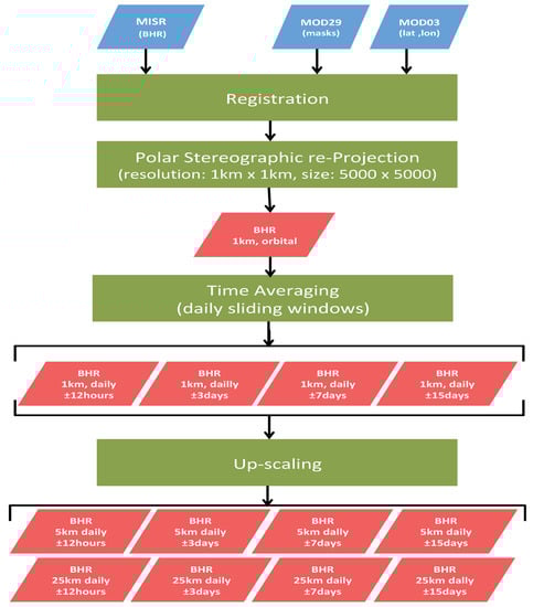
Figure 1.
Production Flowchart (blue: input products; green: process; red: final output products).
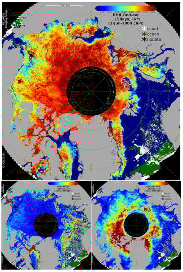
Figure 2.
Sample of the output product (BHR_red, daily, days, 1 km) for 12 June 2000; (top) average; (bottom left) coefficient of variation (standard deviation/average); (bottom right) number of samples.
It is important to note that we do not deal directly here with the creation of either the BHR albedo or the sea-ice mask. The specially processed sea ice MISR albedo was created using a modified algorithm from the standard Rayleigh-only atmospheric correction over the Arctic by JPL and processed at NASA/LaRC. Furthermore, the MODIS sea ice masks already exist in the publicly available NASA DAAC but are stored separately and in different formats and grids. Three main contributions are presented here: (1) creation of significantly cloud free sea ice albedo products from a fusion of two products, specially processed MISR surface albedo and MODIS sea ice mask; (2) evaluation of the accuracy of satellite-derived albedo using in-situ data; (3) study of changes in Arctic sea ice albedo magnitude between 2000 and 2016.
4. Validation
To evaluate the stability and accuracy of the MISR sea ice albedo, we performed a comparison against a tower-based albedometer dataset. These albedometer measurements were obtained from the Alaskan Barrow station (latitude = 71.323N, longitude = 156.607W), which is located on a wide flat coastal area in Northern Alaska, USA, with an elevation close to sea level (around 8 m). These data were provided by the GMD-Radiation group of NOAA/ESRL/GMD/GRAD. Before the ice melts, the area surrounding the Barrow albedometer is very similar to that of sea ice over open water. The height of the albedometer is around 4 m, and given a field of view of 170, the diameter of the albedometer footprint was around 100 m. For further information about this station and the albedometer see https://www.esrl.noaa.gov/gmd/obop/brw/. It should be noted that this is the only long-term station with publicly available albedometer data over the same time-span (and longer) that the authors could locate within the Arctic region.
MISR albedos are not cloud masked over the Barrow station because that station is not located in the open water area, and MOD29 does not include data over any landmass. To overcome this problem, the MISR (single pixel) measurements over Barrow were excluded if (a) the distance to the nearest cloudy pixel was less than 50 km or (b) the acquisition time was less than 45 min to the nearest cloudy measurement of the Barrow station. This filtering of the MISR data allowed us to diminish the risk of moving clouds, and this helped to minimise cloud contamination in this inter-comparison between ground-based and MISR albedo data. Note that the Barrow station data were labeled as cloudy (cloud shadowed) if the ratio of the diffuse radiance to total irradiance component of downwelling radiation was larger than 60%. Note also that only one pixel was considered per MISR overpass, which is the pixel overlapping the Barrow station.
The tower-based measurements were taken every minute and include several variables; however, we were interested in three time series of radiance measurements: total_downwelling, diffuse_downwelling, and total_upwelling. Station albedo could then be computed as follows:
The variable diffuse_downwelling is used to filter station data, especially for labeling clouds (for the preliminary MISR filter as described above) and BHR estimation. As station measurements were acquired over shortwave ([300 nm, 3000 nm]), we calculated a MISR response over the shortwave by linearly combining MISR albedos (BHR) over four narrow spectral bands using Liang’s coefficients [13] as follows:
Tower albedo measurements were screened for cloudy conditions to verify that MISR_BHR values were taken when MISR was cloud free and within 6 min of an MISR overpass. These albedos were time-averaged and matched against the corresponding MISR albedo value. Note that tower measurement are considered cloud free if they have a given time stability and their ratio of diffuse radiance to total incoming irradiance component is low.
Another concern with this inter-comparison study was that MISR’s pixel size (≈1 km) is much larger than the albedometer’s footprint of the Barrow albedometer station (≈100 m), which might lead to a misinterpretation of the results. However, we believe that the location of the Barrow station is representative of the surrounding area (including sea ice) outside the period of ice melting or formation, which is habitually in June to September (see Figure 3). Thus, we limited our comparison of selected pairs (, ) to the presence of ice and snow using a threshold of (0.8, 0.8) as a minimum value before a pair was considered.

Figure 3.
Barrow station; (left) in April; (right) in September (Source: GoogleEarth).
These restrictions on sample collection were applied to MISR and ground data, resulting in a smaller matchup dataset used for this inter-comparison study. Thus, 669 pairs (, ) (out of many thousands) were considered over the 17 years of observation, and from these 669 samples, 119 pairs having high values (bigger than 0.8 for non melted ice) were considered for this inter-comparison. These samples are presented in Figure 4, whereas Figure 5 shows the time series of bias () that was calculated for each year from these well-filtered samples. The variation of the bias is within 5%, which is within the expected uncertainty expected from the calibration uncertainties of 1.5% over the entire time period [30], the expected uncertainties of the tower albedometer Kipp and Zonen CMP21/22 of 2%, and the variability expected from the difference of the FoV of the tower albedometer and the satellite footprint.
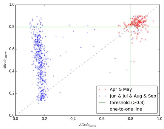
Figure 4.
Pairs of (, ) for the period 2000–2016. Only 119 (out of 669) pairs with values >0.8 were considered. Most of those considered pairs were taken during April and May, when the albedometer (Barrow station) footprint was representative of an MISR resolution cell (and this time period is prior to the ice melting period).
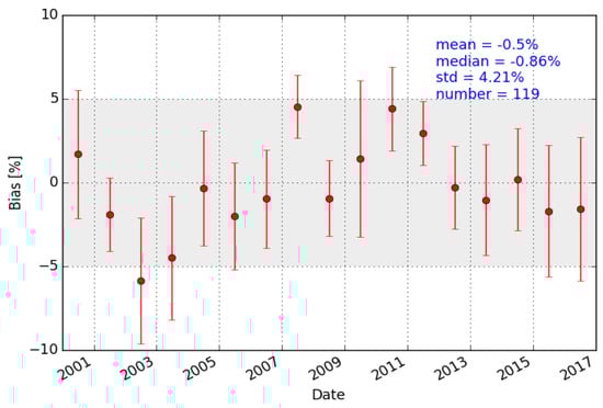
Figure 5.
Bias () over the Barrow station shown as red dots and their associated error bars representing the average bias and standard deviation by year.
The bias has a mean around −0.5% (nearly null), a standard deviation of 4.2%, and a sign that varies every 7–8 years. Thus, even though match-up samples are few in number, they clearly show that the MISR_BHR is very similar to those measured by the albedometer; moreover, this accuracy has not incurred any systematic error or meaningful degradation during the MISR lifetime. Obviously, this study does not provide an absolute assessment of MISR albedos from its four spectral bands, but we believe that the high-quality samples of this comparison study are sufficient to confirm the overall accuracy and stability of the MISR_BHR. In other work over a bright land surface (the calibration site of Railroad Valley Playa, NV, USA), we see values of BRF (bi-directional reflectance factor) from the NASA-CAR instrument in the MISR spectral bands at the various different view angles that are very similar to what we retrieved with the MISR. Thus, we have a high degree of confidence in the retrieved BRFs that go into the albedo calculation [31].
5. Trend Analysis
In this section, before presenting the results of our trend analysis of MISR albedo (BHR shortwave) over Arctic sea ice, we first describe the method that we have employed. However, it is important to mention that we are not dealing here with any direct assessment of climate change. Instead, we believe we have a high quality multiyear satellite-derived sea ice albedo, and the time series shows a continuous reduction of albedo during the last several decades as other studies have indicated, with respect to either the albedo itself [32,33] or related variables such as sea ice melt [34] or thickness [35]. Thus, an overall sea ice albedo variation is shown here to determine whether our sea ice albedo can yield preliminary results that are consistent with the fact that sea ice reflects less and less solar energy from one year to the next.
It is worth noting that, since the Terra satellite has an inclination of , there is a ‘hole’ near the pole. Nevertheless, this gap is tiny in comparison with the rest of the Arctic especially when taking into account the usable area where the solar zenith angle, SZA < ; this trend study is therefore focused on the Arctic region below a latitude of .
The processed BHR 2D-arrays can be stacked into sequential images because all of the products are on the same spatial grid and are co-registered to sub-km accuracy. In fact, and as described in the Production section in this paper, there are three grids—all identical over the covered area but each with a specific spatial resolution (1 km, 5 km, 25 km). For this trend evaluation study, we mainly consider 1 km daily products of two averaging windows: ±15 days and ±7 days.
The idea here is to evaluate this trend in BHR for the same day of the year between 2000 and 2016. Thus, we compute the means and the standard deviations of BHR over the entire Arctic sea for all days and then make a multiyear comparison by day of the year for all of these years. Note that in this study, MISR_BHR is considered when it is either over sea ice or over open water (similar to other studies based on AVHRR). Therefore, a considered pixel in this study is not necessarily related to sea ice; it could also be related to open water (melted sea ice). Other mixtures, such as meltwater ponds, are also possible.
To evaluate the variation of albedo for a given day of year (DoY) over multiple years, we need to be sure that we are comparing the same area. Otherwise, this study will be biased by years in which there are more cloud-free samples. Thus, to overcome this problem of inequality in the number of valid pixels across years, we used a multiyear mask; that is, for a given day of year, pixels are only valid on that day for all years that were considered. It is good to recall that we considered a pixel as valid for a given day and an averaging time window only if that pixel had at least one cloud-free measurement of MISR albedo over its period of averaging. For further clarification, Figure 6 shows a multiyear overview of of August (15 August ± 15 days) before and after applying a multiyear mask. In this example, the area that was varying between km and km becomes a unique and common area ( × km), which is the intersection of all valid areas on 15 August between 2000 and 2016.
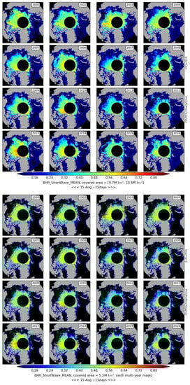
Figure 6.
for 15 August ± 15 days between 2000 and 2016; (top figure) original data having variable area per year; (bottom figure) after multiyear masking, all have the same area. Multiyear masking approach was deployed in our trend analysis.
We computed statistics for six months (April, May, June, July, August, September) for all years between 2000 and 2016 (except for the year 2001 where there were too many missing input data due to a Terra satellite anomaly). Thus, Figure 7 shows the variation of for these six months. In this figure, to show the overall trend, a fitted line is also given by day of year (or by month: on the 15th of each month with an averaging time window of ±15 days):
where and are calculated by DoY for a given spatial resolution and averaging time window.
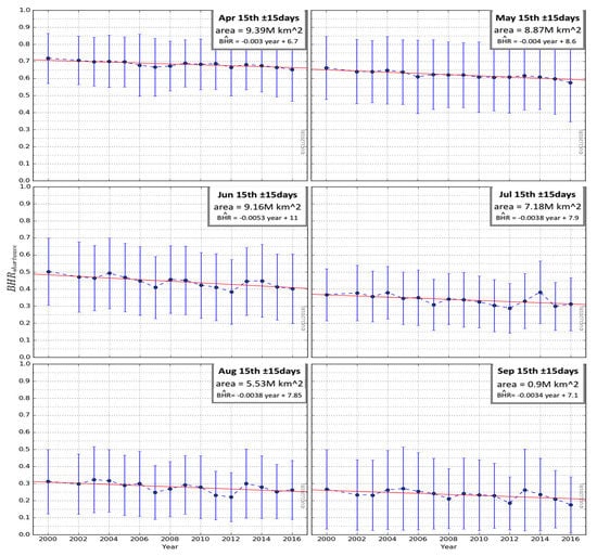
Figure 7.
change by month (15th ± 15 days): April, May, June, July, August, and September.
Moreover, in Figure 7, the total area of valid pixels (in km) is also provided because of the fact that this area does not only vary with cloudiness but also with daylight length, and the variation in the observed area should be taken into consideration before drawing any conclusions.
Statistics over vast areas are more reproducible and less noisy than in small areas. In this way, to compute the overall trend, we applied a weighted average over all yearly trends by day of year in such a way that the weight for each day of the year is its associated area (the wider the area, the more its derived trend is considered). Figure 8 shows a summary of derived trends over all days of the year using two 1 km daily products ( and days). We derived an overall annual change of per year using the daily ± 15 day product and a change of per year using the daily ± 7 day product. However, over the two months of April and May (prior to the ice melting period), the annual change was per year according to the daily ± 15 day product and per year according to the daily ± 7 day product. Note that the annual change for a given day of year (DoY) was computed from the (Equation (4)) as follows:
where and represent the parameters of a fitted trend line (Equation (4)). The weighted average (weight = area [km]) of annual change over an interval of DoYs could then be calculated as follows (for a given spatial resolution and averaging time window):
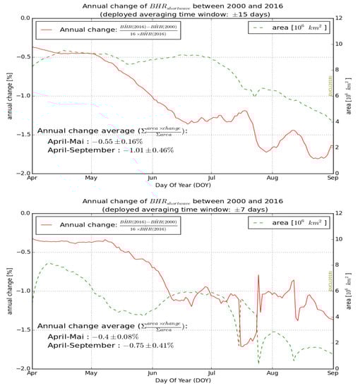
Figure 8.
Annual change of by day of year with their associated area; top: using the 1 km daily ±15 day product; bottom: using the 1 km daily ±7 day product.
This study noticeably demonstrates that our final albedo product is consistent with most modelling studies about the impact of climate change on Arctic sea ice albedo. The 2000–2016 trend for all days and months was negative, with an amplitude varying, generally, between and . Nevertheless, the numbers obtained here differ from those obtained by other studies about the trend of albedo in the Arctic region, namely [33], where the trend was about using the DHR of AVHRR over a different time period [1980–2009]. This difference could be due to the use of DHR instead of BHR, to the effects of cloud contamination in AVHRR, or to the use of a different study period. It could also be due to the fact that AVHRR covers the whole Arctic region, while MISR does not sample above latitude = 84. However, this lack of total coverage of the Arctic is not believed to have any significant impact on the results of this study because, close to the pole, the area affected is very small compared with the whole region covered by sea ice [33].
6. Summary and Conclusions
In this paper, we describe the production process of a new spectral and broadband albedo product for Arctic sea ice. The process consists of combining the MISR_BHR with a MODIS cloud mask and then re-projecting the combined files into three predefined grids over an identical region of 5000 km × 5000 km in size centred on the North Pole (latitude = 90), each one with a specific spatial resolution (1 km, 5 km, 25 km). Next, we describe how we created three daily products, each with a different averaging and sliding time window (±12 h, ±3 days, ±7 days, days). Finally, 12 products were created (3 spatial resolutions times 4 temporal resolutions). Each product includes the mean and standard deviation of the measured BHR during the averaging time window, the number of valid BHR values, and flags (no data, night, land). It should be noted that the input MISR albedo product did contain an estimated uncertainty value, but these values were so small they are not included here.
This paper also presented a comparison study against tower-based measurements. The ground truth data provided by a well-calibrated albedometer of the Barrow station (of NOAA/ESRL/GMD/GRAD), which is located in a coastal area of Northern Alaska and whose elevation is close to sea level. The albedometer data were filtered in such a way that only cloud-free and simultaneous measurements with MISR overpass dates/time (12 min averaging) were considered. The comparison clearly demonstrated that MISR albedo appears accurate and does not seem to incur any significant time-dependent degradation or miscalibration.
The trend of sea ice albedo over the whole Arctic was also evaluated, although the MISR albedo does not cover regions above a latitude of . However, this will have a negligible impact in this trend evaluation study because of the small size of the region remaining compared with that of the whole area of the Arctic. We present here the trend for each month between April and September using the 1 km monthly product, which is represented by the daily product on the 15th of each month with an averaging time of ±15 days (Figure 7). However, the whole trend analysis study was based on two daily 1 km products: ±15 days and ±7 days (Figure 8).
We note from Figure 7 that the standard variation becomes larger during the melting period of sea ice and shorter prior to that period. This is because the pixel could either be ice or water during the averaging time window ( h, days, days, days), and this mixture occurs more frequently during the ice melting period. Nevertheless, both averaging windows that we used in our trend analysis ( days, days) did not lead to any significantly different results with regard to albedo reduction (Figure 8).
The timeframe of the trend analysis study covered the entire daylight period over the Arctic between 2000 and 2016, except 2001. The results revealed that the BHR [April–May] over sea ice incurs an annual reduction of per year according to the 1 km daily product of the day averaging time window and according to the product of the day averaging time window (also 1 km daily). It appears that the sign of the trend was negative. We can say that the results of this study are consistent with most of the comparable studies on the assumption that there is a continuous reduction in sea ice albedo, but it differs in the magnitude of this trend. This difference could be due to the fact that satellite data that were used by previous studies were cloud-contaminated (e.g., AVHRR) or to the fact that albedo (BHR or DHR) was not well retrieved, especially for AVHRR or any other albedo products that require multidate cloud-free observation from satellites. However, as we have already mentioned in the previous section, this trend evaluation is very preliminary and more in-depth investigation using our sea ice albedo should assist climate scientists.
We believe that the high quality and the high resolution of our products will be of great benefit to the climate change community and especially to those who are interested in sea ice albedo and derived variables and their feedback with the climate system. Furthermore, the format and structure that our products come with make it easy to derive up-scaled (spatial or temporal) products to fit specific requirements. Moreover, the promising results that this paper presented in terms of feasibility and accuracy and in terms of climate change trend evaluation have encouraged us to create similar products for Antarctica. This will be the subject of our next report. Last but not least, we hope that our process will be adopted for continuous production because the actual available dataset does not cover 2017 and beyond. The products are available for download from the QA4ECV website (www.qa4ecv.eu) and in the future will be assigned a DOI.
Author Contributions
Conceptualization, J.-P.M. (Jan-Peter Muller) and S.K. (Said Kharbouche); methodology, S.K.; software, S.K.; validation, J.-P.M., S.K.; formal analysis, S.K.; investigation, SK; data curation, J.-P.M.; writing original draft preparation, S.K.; writing review and editing, J.-P.M.; visualization, S.K.; supervision, J.-P.M.; project administration, J.-P.M.; funding acquisition, J.-P.M.
Funding
This work was supported by the QA4ECV project www.QA4ECV.eu, of the European Union’s Seventh Framework Programme (FP7/2007–2013) under grant agreement number 607405.
Acknowledgments
We thank our colleagues at JPL and NASA LaRC for processing the MISR data, especially Sebastian Val and Steve Protack, respectively. We also acknowledge the GMD-Radiation group of NOAA/ESRL/GMD/GRAD for providing us with the in situ data.
Conflicts of Interest
The authors declare that there is no conflict of interest and, the founding sponsors had no role in the design of the study; in the collection, analyses, or interpretation of data; in the writing of the manuscript; or in the decision to publish the results.
Abbreviations
The following abbreviations are used in this manuscript:
| AVHRR | Advanced Very High Resolution Radiometer |
| BHR | Bi-Hemispherical Reflectance (for the case of White Sky Albedo) |
| DHR | Directional Hemispherical Reflectance (Black Sky Albedo) |
| MISR | Multi-angle Imaging SpectroRadiometer |
| MODIS | MODerate Resolution Imaging Spectroradiometer |
| MOD29 | sea ice product of MODIS |
| MOD03 | geolocation product of MODIS |
Appendix A. Data
The data in netCDF4 (CF) format can be downloaded from: http://www.qa4ecv-land.eu/get-polar-sea-ice.php. Browse still and animated images are available via http://www.qa4ecv.eu. Also available at http://catalogue.ceda.ac.uk/uuid/38296ae73f3b44f5b8d66dcc3ed398bd.
Appendix B. Assessment of MOD29 Cloud Mask
The MOD29 cloud mask which is formed from the MOD35 cloud mask has been assessed using CALIPSO data with MODIS in the A-train, and the results are shown below. Note the 90% hit-rate of MOD35 with CALIPSO cloud detection (see Figure A1).

Figure A1.
MOD35 hit-rates with CALIPSO over sea-ice from 2012 to 2016. (Frey and Ackerman, private communication, 2018).
Figure A1.
MOD35 hit-rates with CALIPSO over sea-ice from 2012 to 2016. (Frey and Ackerman, private communication, 2018).

References
- Hall, A. The role of surface albedo feedback in climate. J. Clim. 2004, 17, 1550–1568. [Google Scholar] [CrossRef]
- Bojinski, S.; Verstraete, M.; Peterson, T.C.; Richter, C.; Simmons, A.; Zemp, M. The concept of essential climate variables in support of climate research, applications, and policy. Bull. Am. Meteorol. Soc. 2014, 95, 1431–1443. [Google Scholar] [CrossRef]
- Holland, M.M.; Bitz, C.M. Polar amplification of climate change in coupled models. Clim. Dyn. 2003, 21, 221–232. [Google Scholar] [CrossRef]
- Hall, A.; Qu, X. Using the current seasonal cycle to constrain snow albedo feedback in future climate change. Geophys. Res. Lett. 2006, 33. [Google Scholar] [CrossRef]
- Perovich, D.K.; Polashenski, C. Albedo evolution of seasonal Arctic sea ice. Geophys. Res. Lett. 2012, 39. [Google Scholar] [CrossRef]
- Holland, M.M.; Bitz, C.M.; Hunke, E.C.; Lipscomb, W.H.; Schramm, J.L. Influence of the sea ice thickness distribution on polar climate in CCSM3. J. Clim. 2006, 19, 2398–2414. [Google Scholar] [CrossRef]
- Eisenman, I.; Untersteiner, N.; Wettlaufer, J. On the reliability of simulated Arctic sea ice in global climate models. Geophys. Res. Lett. 2007, 34. [Google Scholar] [CrossRef]
- Stroeve, J.C.; Kattsov, V.; Barrett, A.; Serreze, M.; Pavlova, T.; Holland, M.; Meier, W.N. Trends in Arctic sea ice extent from CMIP5, CMIP3 and observations. Geophys. Res. Lett. 2012, 39. [Google Scholar] [CrossRef]
- Winton, M. Amplified Arctic climate change: What does surface albedo feedback have to do with it? Geophys. Res. Lett. 2006, 33. [Google Scholar] [CrossRef]
- Perovich, D.K.; Light, B.; Eicken, H.; Jones, K.F.; Runciman, K.; Nghiem, S.V. Increasing solar heating of the Arctic Ocean and adjacent seas, 1979–2005: Attribution and role in the ice-albedo feedback. Geophys. Res. Lett. 2007, 34. [Google Scholar] [CrossRef]
- Belward, A.S.; Skøien, J.O. Who launched what, when and why; trends in global land-cover observation capacity from civilian earth observation satellites. ISPRS J. Photogramm. Remote Sens. 2015, 103, 115–128. [Google Scholar] [CrossRef]
- Strahler, A.H.; Muller, J.; Lucht, W.; Schaaf, C.; Tsang, T.; Gao, F.; Li, X.; Lewis, P.; Barnsley, M.J. MODIS BRDF/albedo product: Algorithm theoretical basis document version 5.0. MODIS Doc. 1999, 23, 42–47. [Google Scholar]
- Liang, S. Narrowband to broadband conversions of land surface albedo I: Algorithms. Remote Sens. Environ. 2001, 76, 213–238. [Google Scholar] [CrossRef]
- Muller, J.P.; López, G.; Watson, G.; Shane, N.; Kennedy, T.; Yuen, P.; Lewis, P.; Fischer, J.; Guanter, L.; Domench, C.; et al. The ESA GlobAlbedo Project for mapping the Earth’s land surface albedo for 15 Years from European Sensors. Geophys. Res. Abstr. 2012, 13, 10969. [Google Scholar]
- Diner, D.J.; Beckert, J.C.; Reilly, T.H.; Bruegge, C.J.; Conel, J.E.; Kahn, R.A.; Martonchik, J.V.; Ackerman, T.P.; Davies, R.; Gerstl, S.A.; et al. Multi-angle Imaging SpectroRadiometer (MISR) instrument description and experiment overview. IEEE Trans. Geosci. Remote Sens. 1998, 36, 1072–1087. [Google Scholar] [CrossRef]
- Karlsson, K.G.; Riihelä, A.; Müller, R.; Meirink, J.; Sedlar, J.; Stengel, M.; Lockhoff, M.; Trentmann, J.; Kaspar, F.; Hollmann, R.; et al. CLARA-A1: A cloud, albedo, and radiation dataset from 28 yr of global AVHRR data. Atmos. Chem. Phys. 2013, 13, 5351–5367. [Google Scholar] [CrossRef]
- Karlsson, K.G.; Anttila, K.; Trentmann, J.; Stengel, M.; Meirink, J.F.; Devasthale, A.; Hanschmann, T.; Kothe, S.; Jääskeläinen, E.; Sedlar, J.; et al. CLARA-A2: The second edition of the CM SAF cloud and radiation data record from 34 years of global AVHRR data. Atmos. Chem. Phys. 2017, 17, 5809–5828. [Google Scholar] [CrossRef]
- Aoki, T.; Aoki, T.; Fukabori, M.; Hachikubo, A.; Tachibana, Y.; Nishio, F. Effects of snow physical parameters on spectral albedo and bidirectional reflectance of snow surface. J. Geophys. Res. Atmos. 2000, 105, 10219–10236. [Google Scholar] [CrossRef]
- Zhao, T.X.P.; Chan, P.K.; Heidinger, A.K. A global survey of the effect of cloud contamination on the aerosol optical thickness and its long-term trend derived from operational AVHRR satellite observations. J. Geophys. Res. Atmos. 2013, 118, 2849–2857. [Google Scholar] [CrossRef]
- Peltoniemi, J.I.; Kaasalainen, S.; Naranen, J.; Matikainen, L.; Piironen, J. Measurement of directional and spectral signatures of light reflectance by snow. IEEE Trans. Geosci. Remote Sens. 2005, 43, 2294–2304. [Google Scholar] [CrossRef]
- Warren, S.G.; Brandt, R.E.; O’Rawe Hinton, P. Effect of surface roughness on bidirectional reflectance of Antarctic snow. J. Geophys. Res. Planets 1998, 103, 25789–25807. [Google Scholar] [CrossRef]
- Kay, J.E.; Gettelman, A. Cloud influence on and response to seasonal Arctic sea ice loss. J. Geophys. Res. Atmos. 2009, 114. [Google Scholar] [CrossRef]
- Riggs, G.A.; Hall, D.K. MODIS/Terra Sea Ice Extent 5-Min L2 Swath 1km, Version 6. [MOD29]; Technical Report; NASA National Snow and Ice Data Center Distributed Active Archive Center: Boulder, CO, USA, 2015. [Google Scholar] [CrossRef]
- Jovanovic, V.; Miller, K.; Rheingans, B.; Moroney, C. MISR Science Data Product Guide; Jet Propulsion Laboratory, California Institute of Technology: Pasadena, CA, USA, 2012. [Google Scholar]
- Martonchik, J.V.; Diner, D.J.; Pinty, B.; Verstraete, M.M.; Myneni, R.B.; Knyazikhin, Y.; Gordon, H.R. Determination of land and ocean reflective, radiative, and biophysical properties using multiangle imaging. IEEE Trans. Geosci. Remote Sens. 1998, 36, 1266–1281. [Google Scholar] [CrossRef]
- Ackerman, S.; Holz, R.; Frey, R.; Eloranta, E.; Maddux, B.; McGill, M. Cloud detection with MODIS. Part II: Validation. J. Atmos. Ocean. Technol. 2008, 25, 1073–1086. [Google Scholar] [CrossRef]
- Schaepman-Strub, G.; Schaepman, M.; Painter, T.; Dangel, S.; Martonchik, J. Reflectance quantities in optical remote sensing—Definitions and case studies. Remote Sens. Environ. 2006, 103, 27–42. [Google Scholar] [CrossRef]
- Herber, A.; Thomason, L.W.; Gernandt, H.; Leiterer, U.; Nagel, D.; Schulz, K.H.; Kaptur, J.; Albrecht, T.; Notholt, J. Continuous day and night aerosol optical depth observations in the Arctic between 1991 and 1999. J. Geophys. Res. Atmos. 2002, 107. [Google Scholar] [CrossRef]
- Pinty, B.; Lattanzio, A.; Martonchik, J.V.; Verstraete, M.M.; Gobron, N.; Taberner, M.; Widlowski, J.L.; Dickinson, R.E.; Govaerts, Y. Coupling diffuse sky radiation and surface albedo. J. Atmos. Sci. 2005, 62, 2580–2591. [Google Scholar] [CrossRef]
- Bruegge, C.J.; Val, S.; Diner, D.J.; Jovanovic, V.; Gray, E.; Di Girolamo, L.; Zhao, G. Radiometric stability of the Multi-angle Imaging SpectroRadiometer (MISR) following 15 years on-orbit. In Proceedings of the SPIE Optical Engineering and Applications, San Diego, CA, USA, 17–21 August 2014. [Google Scholar]
- Kharbouche, S.; Muller, J.P.; Gatebe, C.K.; Scanlon, T.; Banks, A.C. Assessment of Satellite-Derived Surface Reflectances by NASA’s CAR Airborne Radiometer over Railroad Valley Playa. Remote Sens. 2017, 9, 562. [Google Scholar] [CrossRef]
- Laine, V. Arctic sea ice regional albedo variability and trends, 1982–1998. J. Geophys. Res. Oceans 2004, 109. [Google Scholar] [CrossRef]
- Riihelä, A.; Manninen, T.; Laine, V. Observed changes in the albedo of the Arctic sea-ice zone for the period 1982–2009. Nat. Clim. Chang. 2013, 3, 895–898. [Google Scholar] [CrossRef]
- Stroeve, J.; Markus, T.; Boisvert, L.; Miller, J.; Barrett, A. Changes in Arctic melt season and implications for sea ice loss. Geophys. Res. Lett. 2014, 41, 1216–1225. [Google Scholar] [CrossRef]
- Laxon, S.; Peacock, N.; Smith, D. High interannual variability of sea ice thickness in the Arctic region. Nature 2003, 425, 947–950. [Google Scholar] [CrossRef] [PubMed]


© 2018 by the authors. Licensee MDPI, Basel, Switzerland. This article is an open access article distributed under the terms and conditions of the Creative Commons Attribution (CC BY) license (http://creativecommons.org/licenses/by/4.0/).