Analyzing the Relationship between Developed Land Area and Nighttime Light Emissions of 36 Chinese Cities


Abstract

1. Introduction
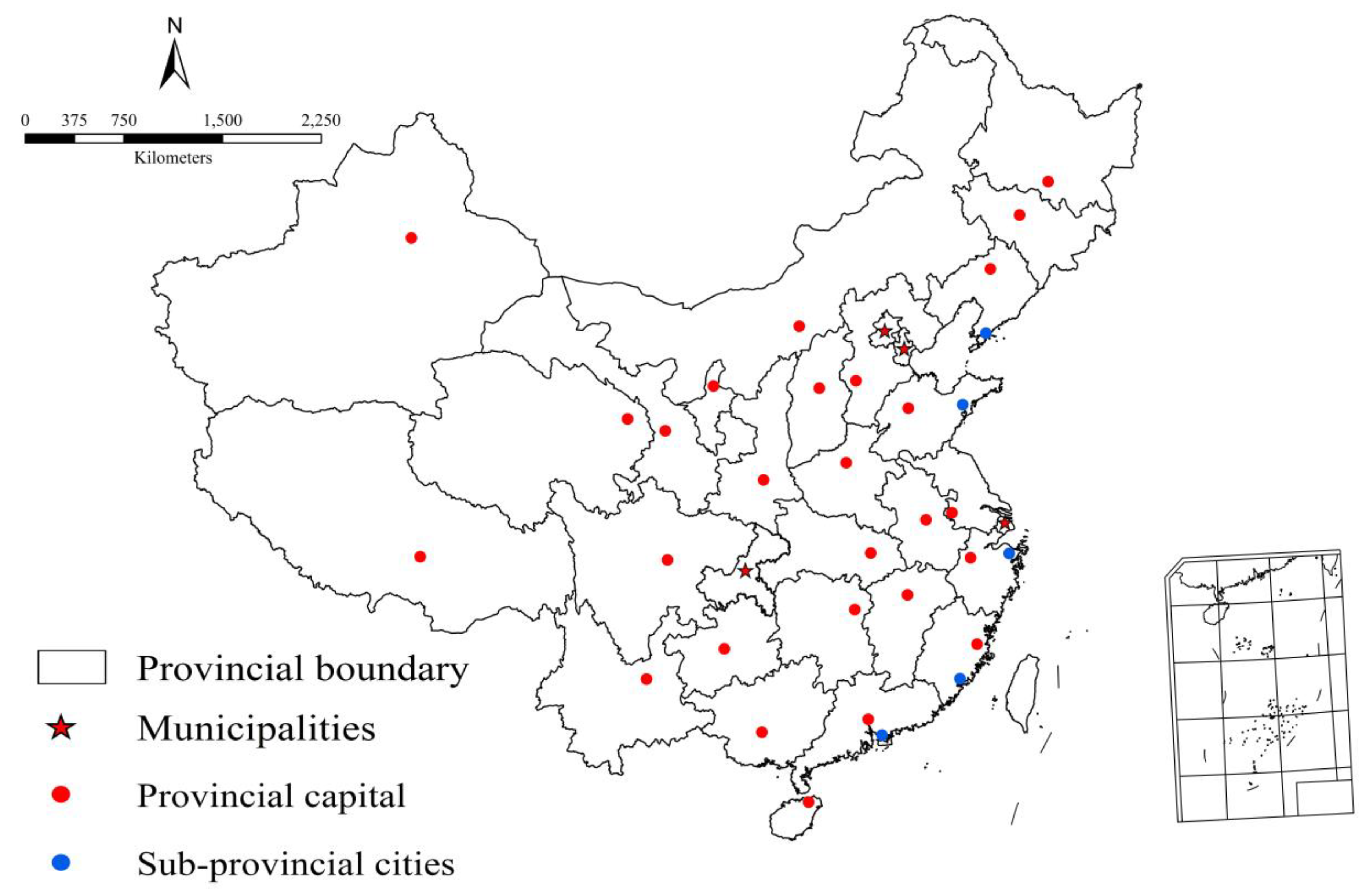
2. Study Area
3. Materials and Methods
3.1. Datasets
3.2. Methods
3.2.1. Data Preprocessing
3.2.2. Generation of Enhanced DMSP/OLS Data
3.2.3. Measurement of NTLE
3.2.4. Statistical Analysis
4. Results
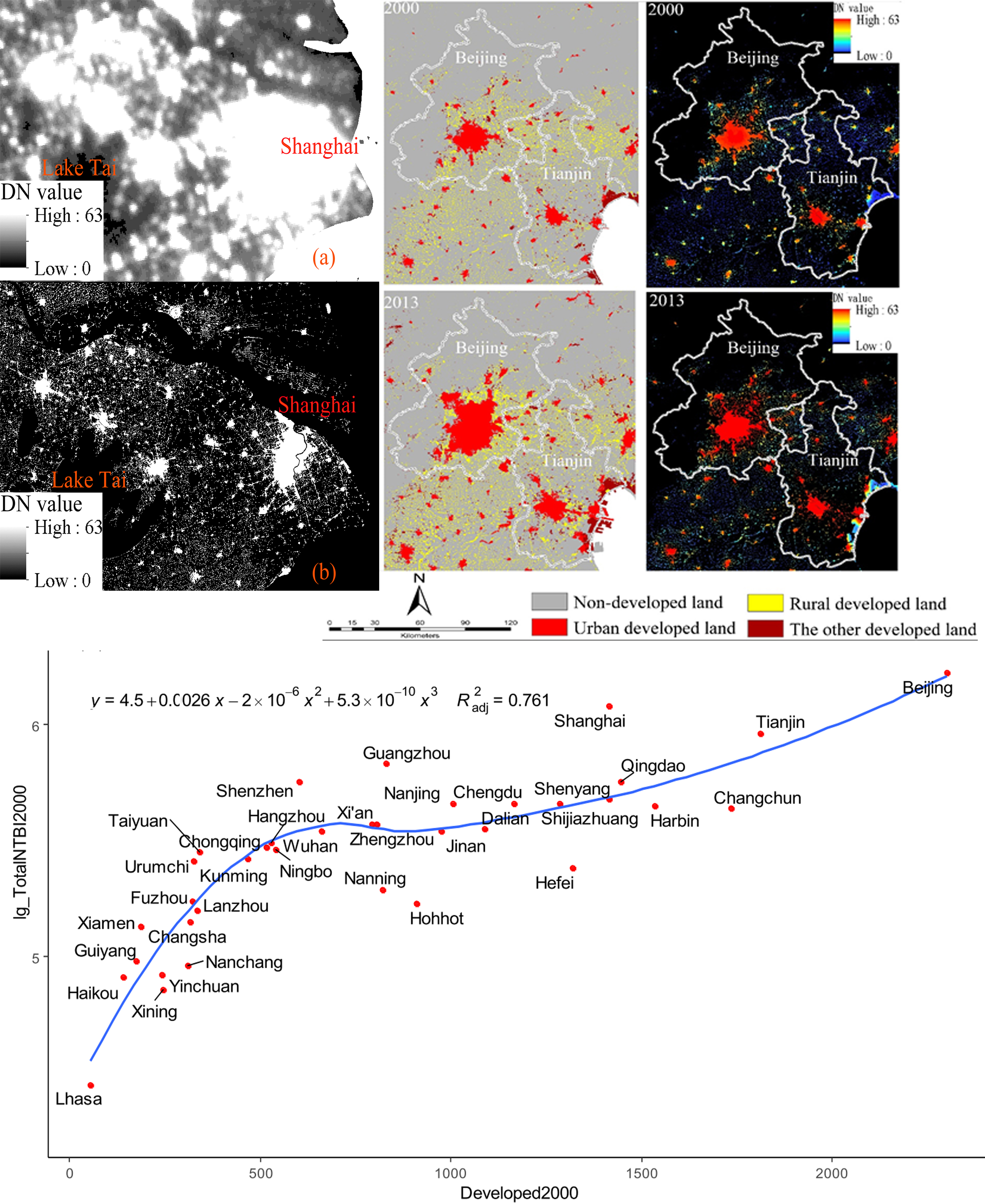
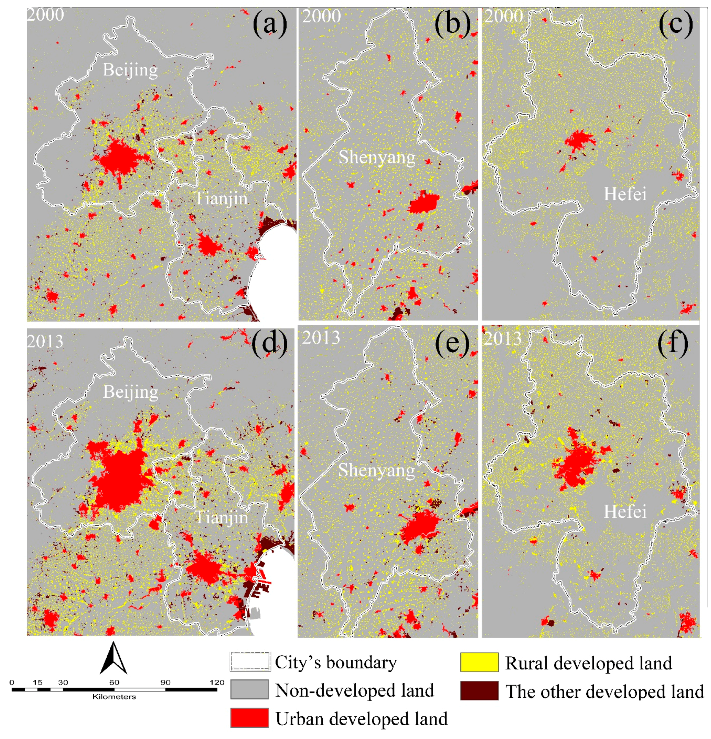
4.1. Synaptic Analysis of Growth Patterns of Developed Land
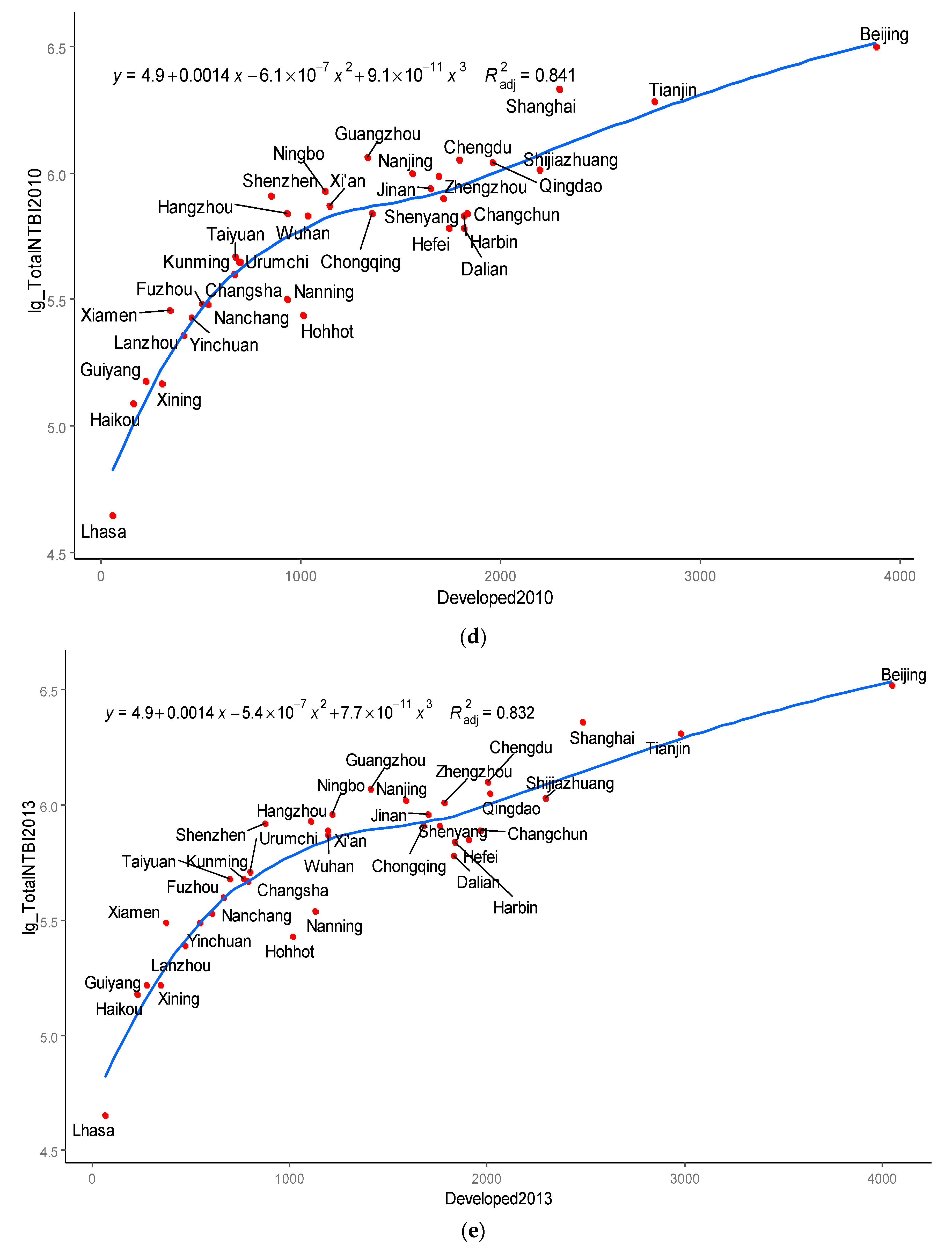
4.2. The Dynamics of NTBI in Response to Developed Land Growth
4.3. Driving Factors Underlying the Relationship Between Developed Land Area and Associated TotalNTBI
5. Discussion
5.1. Uncertainty in Enhanced DMSP/OLS Due to Data Sources and Methods
5.2. Relationship Between Developed Land Area and Associated NTLEs
5.3. Implications
6. Conclusions
Supplementary Materials
Author Contributions
Funding
Acknowledgments
Conflicts of Interest
References
- United Nations. 2018 Revision of World Urbanization Prospects. Available online: https://www.un.org/development/desa/publications/2018-revision-of-world-urbanization-prospects.html (accessed on 20 November 2018).
- Ellis, E.C.; Kaplan, J.O.; Fuller, D.Q.; Vavrus, S.; Goldewijk, K.K.; Verburg, P.H. Used planet: A global history. Proc. Natl. Acad. Sci. USA 2013, 110, 7978–7985. [Google Scholar] [CrossRef] [PubMed]
- Mcdonald, R.I.; Weber, K.; Padowski, J.; Flörke, M.; Schneider, C.; Green, P.A.; Gleeson, T.; Eckman, S.; Lehner, B.; Balk, D.; et al. Water on an urban planet: Urbanization and the reach of urban water infrastructure. Glob. Environ. Chang. 2014, 27, 96–105. [Google Scholar] [CrossRef]
- Bagan, H.; Yamagata, Y. Analysis of urban growth and estimating population density using satellite images of nighttime lights and land-use and population data. GISci. Remote Sens. 2015, 52, 765–780. [Google Scholar] [CrossRef]
- Doll, C.N.H.; Pachauri, S. Estimating rural populations without access to electricity in developing countries through night-time light satellite imagery. Energy Policy 2010, 38, 5661–5670. [Google Scholar] [CrossRef]
- Gibson, J.; Boe-Gibson, G.; Stichbury, G. Urban land expansion in India 1992–2012. Food Policy 2015, 56, 100–113. [Google Scholar] [CrossRef]
- Kontgis, C.; Schneider, A.; Fox, J.; Saksena, S.; Spencer, J.H.; Castrence, M. Monitoring peri-urbanization in the greater Ho Chi Minh City metropolitan area. Appl. Geogr. 2014, 53, 377–388. [Google Scholar] [CrossRef]
- Sharma, R.C.; Tateishi, R.; Hara, K.; Gharechelou, S.; Iizuka, K. Global mapping of urban built-up areas of year 2014 by combining MODIS multispectral data with VIIRS nighttime light data. Int. J. Digit. Earth 2016, 9, 1004–1020. [Google Scholar] [CrossRef]
- Small, C.; Pozzi, F.; Elvidge, C.D. Spatial analysis of global urban extent from DMSP-OLS night lights. Remote Sens. Environ. 2005, 96, 277–291. [Google Scholar] [CrossRef]
- Taubenböck, H.; Wiesner, M.; Felbier, A.; Marconcini, M.; Esch, T.; Dech, S. New dimensions of urban landscapes: The spatio-temporal evolution from a polynuclei area to a mega-region based on remote sensing data. Appl. Geogr. 2014, 47, 137–153. [Google Scholar] [CrossRef]
- Zhou, N.; Hubacek, K.; Roberts, M. Analysis of spatial patterns of urban growth across South Asia using DMSP-OLS nighttime lights data. Appl. Geogr. 2015, 63, 292–303. [Google Scholar] [CrossRef]
- Zhou, Y.; Smith, S.J.; Elvidge, C.D.; Zhao, K.; Thomson, A.; Imhoff, M. A cluster-based method to map urban area from DMSP/OLS nightlights. Remote Sens. Environ. 2014, 147, 173–185. [Google Scholar] [CrossRef]
- Keola, S.; Andersson, M.; Hall, O. Monitoring economic development from space: Using nighttime light and land cover data to measure economic growth. World Dev. 2015, 66, 322–334. [Google Scholar] [CrossRef]
- Corbane, C.; Kemper, T.; Freire, S.; Louvrier, C.; Pesaresi, M. Monitoring the Syrian Humanitarian Crisis with the JRC’s Global Human Settlement Layer and Night-Time Satellite Data; Publications Office of the European Union: Luxembourg, 2016; pp. 1–14. [Google Scholar]
- Witmer, F.W.; O’Loughlin, J. Detecting the effects of wars in the caucasus regions of Russia and Georgia using radiometrically normalized DMSP-OLS nighttime lights imagery. Mapp. Sci. Rem. Sens. 2011, 48, 478–500. [Google Scholar] [CrossRef]
- Li, X.; Li, D.; Xu, H.; Wu, C. Intercalibration between DMSP/OLS and VIIRS night-time light images to evaluate city light dynamics of Syria’s major human settlement during Syrian Civil War. Int. J. Remote Sens. 2017, 38, 5934–5951. [Google Scholar] [CrossRef]
- Ghosh, T.; Anderson, S.J.; Elvidge, C.D.; Sutton, P.C. Using nighttime satellite imagery as a proxy measure of human well-being. Sustainability 2013, 5, 4988–5019. [Google Scholar] [CrossRef]
- Huang, X.; Schneider, A.; Friedl, M.A. Mapping sub-pixel urban expansion in China using MODIS and DMSP/OLS nighttime lights. Remote Sens. Environ. 2016, 175, 92–108. [Google Scholar] [CrossRef]
- Su, Y.; Chen, X.; Wang, C.; Zhang, H.; Liao, J.; Ye, Y.; Wang, C. A new method for extracting built-up urban areas using DMSP-OLS nighttime stable lights: A case study in the Pearl River Delta, southern China. Mapp. Remote Sens. 2015, 52, 218–238. [Google Scholar] [CrossRef]
- Wang, L. Object-based spatial cluster analysis of urban landscape pattern using nighttime light satellite images: A case study of China. Int. J. Geogr. Inf. Sci. 2014, 28, 2328–2355. [Google Scholar]
- Wu, W.; Zhao, H.; Jiang, S. A Zipf’s Law-Based Method for Mapping Urban Areas Using NPP-VIIRS Nighttime Light Data. Remote Sens. 2018, 10, 130. [Google Scholar] [CrossRef]
- Zheng, Q.; Zeng, Y.; Deng, J.; Wang, K.; Jiang, R.; Ye, Z. “Ghost cities” identification using multi-source remote sensing datasets: A case study in Yangtze river delta. Appl. Geogr. 2017, 80, 112–121. [Google Scholar] [CrossRef]
- Song, G.; Yu, M.; Liu, S.; Zhang, S. A dynamic model for population mapping: A methodology integrating a Monte Carlo simulation with vegetation-adjusted night-time light images. Int. J. Remote Sens. 2015, 36, 4054–4068. [Google Scholar] [CrossRef]
- Zhuo, L.; Ichinose, T.; Zheng, J.; Chen, J.; Shi, P.J.; Li, X. Modelling the population density of China at the pixel level based on DMSP/OLS non-radiance-calibrated night-time light images. Int. J. Remote Sens. 2009, 30, 1003–1018. [Google Scholar] [CrossRef]
- Dai, Z.; Hu, Y.; Zhao, G. The suitability of different nighttime light data for GDP estimation at different spatial scales and regional levels. Sustainability 2017, 9, 305. [Google Scholar] [CrossRef]
- Li, C.; Li, G.; Zhu, Y.; Ge, Y.; Wu, Y. A likelihood-based spatial statistical transformation model (LBSSTM) of regional using DMSP/OLS time-series nighttime light imagery. Spat. Stat. 2017, 21, 421–439. [Google Scholar] [CrossRef]
- Ma, T.; Zhou, C.; Pei, T.; Haynie, S.; Fan, J. Responses of Suomi-NPP VIIRS-derived nighttime lights to socioeconomic activity in China’s cities. Remote Sens. Lett. 2014, 5, 165–174. [Google Scholar] [CrossRef]
- Wang, W.; Cheng, H.; Zhang, L. Poverty assessment using DMSP/OLS night-time light satellite imagery at a provincial scale in China. Adv. Space Res. 2012, 49, 1253–1264. [Google Scholar] [CrossRef]
- Wu, R.; Yang, D.; Dong, J.; Zhang, L.; Xia, F. Regional Inequality in China Based on NPP-VIIRS Night-Time Light Imagery. Remote Sens. 2018, 10, 240. [Google Scholar] [CrossRef]
- Kuffer, M.; Pfeffer, K.; Sliuzas, R.; Taubenböck, H.; Baud, I.; Maarseveen, M.V. Capturing the urban divide in nighttime light images from the international space station. IEEE J. Sel. Top. Appl. Earth Obs. Remote Sens. 2018, 99, 1–9. [Google Scholar] [CrossRef]
- China National Statistical Bureau. China National Statistical Yearbook 2014; China Statistical Press: Beijing, China, 2014.
- Elvidge, C.; Keith, D.; Tuttle, B.; Baugh, K. Spectral identification of lighting type and character. Sensors 2010, 10, 3961–3988. [Google Scholar] [CrossRef] [PubMed]
- Zhang, Q.; Seto, K.C. Mapping urbanization dynamics at regional and global scales using multi-temporal DMSP/OLS nighttime light data. Remote Sens. Environ. 2011, 115, 2320–2329. [Google Scholar] [CrossRef]
- Elvidge, C.D.; Ziskin, D.; Baugh, K.E.; Tuttle, B.T.; Ghosh, T.; Pack, D.W.; Erwin, E.H.; Zhizhin, M. A fifteen-year record of global natural gas flaring derived from satellite data. Energies 2009, 2, 595–622. [Google Scholar] [CrossRef]
- General Administration of Quality Supervision, Inspection and Quarantine of China; Standardiation Administration of China. National Standard for Current Land Use Classification (GB/T 21010-2007); Standards Press of China: Beijing, China, 2017.
- Huang, Q.; Yang, X.; Gao, B.; Yang, Y.; Zhao, Y. Application of DMSP/OLS Nighttime Light Images: A Meta-Analysis and a Systematic Literature Review. Remote Sens. 2014, 6, 6844–6866. [Google Scholar] [CrossRef]
- Croissant, Y.; Millo, G. Panel data econometrics in R: The PLM package. J. Stat. Softw. 2008, 27, 1–43. [Google Scholar] [CrossRef]
- Zhang, Q.; Pandey, B.; Seto, K.C. A robust method to generate a consistent time series from DMSP/OLS nighttime light data. IEEE Trans. Geosci. Remote Sens. 2016, 54, 5821–5831. [Google Scholar] [CrossRef]
- Yao, Y.; Chen, D.; Chen, L.; Wang, H.; Guan, Q. A time series of urban extent in China using DSMP/OLS nighttime light data. PLoS ONE 2018, 13, e0198189. [Google Scholar] [CrossRef] [PubMed]
- Elvidge, C.D.; Tuttle, B.T.; Sutton, P.C.; Baugh, K.E.; Howard, A.T.; Milesi, C.; Bhaduri, B.; Nemani, R. Global Distribution and Density of Constructed Impervious Surfaces. Sensors 2007, 7, 1962–1979. [Google Scholar] [CrossRef] [PubMed]
- Henderson, M.; Yeh, E.T.; Gong, P.; Elvidge, C.; Baugh, K. Validation of urban boundaries derived from global night-time satellite imagery. Int. J. Remote Sens. 2003, 24, 595–609. [Google Scholar] [CrossRef]
- Amaral, S.; Monteiro, A.M.; Câmara, G.; Quintanilha, J.A. DMSP/OLS night-time light imagery for urban population estimates in the Brazilian Amazon. Int. J. Remote Sens. 2006, 27, 855–870. [Google Scholar] [CrossRef]
- Florida, R.; Mellander, C.; Gulden, T. Global metropolis: Assessing economic activity in urban centers based on nighttime satellite images. Prof. Geogr. 2012, 64, 178–187. [Google Scholar] [CrossRef]
- Gao, B.; Huang, Q.; He, C.; Sun, Z.; Zhang, D. How does sprawl differ across cities in China? A multi-scale investigation using nighttime light and census data. Landsc. Urban Plan. 2016, 148, 89–98. [Google Scholar] [CrossRef]
- Lo, C.P. Urban indicators of China from radiance-calibrated digital DMSP/OLS nighttime images. Ann. Assoc. Am. Geogr. 2002, 92, 225–240. [Google Scholar] [CrossRef]
- Moreno, E.L.; Blanco, Z.G. Ghost cities and empty houses: Wasted prosperity. Am. Int. J. Soc. Sci. 2014, 3, 207–216. [Google Scholar]
- Sutton, P.C.; Cova, T.J.; Elvidge, C.D. Mapping “exurbia” in the conterminous United States using nighttime satellite imagery. Geocarto Int. 2006, 21, 39–45. [Google Scholar] [CrossRef]
- Wei, Y.D.; Li, H.; Yue, W. Urban land expansion and regional inequality in transitional China. Landsc. Urban Plan. 2017, 163, 17–31. [Google Scholar] [CrossRef]
- Huang, H.; Wei, Y.D. Spatial inequality of foreign direct investment in China: Institutional change, agglomeration economies, and market access. Appl. Geogr. 2016, 69, 99–111. [Google Scholar] [CrossRef]
- Xue, L. Study on the inner-decaying village and the Countermeasures with Jiangsu province as the case. City Plan. Rev. 2001, 25, 8–13. [Google Scholar]
- Jiang, C. Exploration on the Governance for Guangzhou’s “Hollow Villages”. In Proceedings of the 4th International Conference on Education and Education Management, Singapore, 8–9 December 2014; pp. 66–70. [Google Scholar]
- Chen, J.; Yue, Y.D. Industry agglomeration and industrial migration in China’s industrialization. Syst. Eng. 2013, 31, 92–97. [Google Scholar]
- Huang, X.F.; Yang, D. Dose industrial transfer policy contribute to the convergence between regions: An analysis based on the regression discontinuity of county data from Guangdong. Int. Econ. Trade Res. 2017, 33, 101–112. [Google Scholar]
- Lu, H.Y. Structural adjustment trend in Pearl River Delta under the background of industrial evolution and financial crisis. Forward Pos. Econ. 2009, 9, 25–33. [Google Scholar]
- Xu, D.Y.; Liang, Q. An analysis of the “push” and “pull” of industrial transfer in Pearl River Delta. J. Cent. Univ. Finan. Econ. 2011, 1, 68–73. [Google Scholar]
- Yang, G. Comment on the industry selection and spatial layout of “Great South Hunan” under the background of industrial transfer. Econ. Geogr. 2014, 34, 178. [Google Scholar]
- Sorace, C.; Hurst, W. China’s phantom urbanisation and the pathology of ghost cities. Soc. Sci. Electron. Publ. 2016, 46, 1–19. [Google Scholar] [CrossRef]


| Geographical Zoning | City | Province | Prefecture Rank | Population | GDP | Agr_Pop | Agr_GDP |
|---|---|---|---|---|---|---|---|
| Northern China | Beijing | - | Municipality | 21.148 | 1.950 | 0.123 | 0.578 |
| Tianjin | - | Municipality | 14.722 | 1.437 | 0.096 | 0.362 | |
| Shijiazhuang | Hebei | Provincial capital | 10.032 | 0.491 | 0.015 | 0.045 | |
| Taiyuan | Shanxi | Provincial capital | 3.675 | 0.241 | 0.029 | 0.087 | |
| Hohhot | Inner Mongolia | Provincial capital | 3.001 | 0.271 | 0.019 | 0.070 | |
| Northeastern China | Shenyang | Liaoning | Provincial capital | 8.257 | 0.716 | 0.046 | 0.081 |
| Dalian | Liaoning | sub-Provincial city | 6.943 | 0.727 | 0.047 | 0.110 | |
| Changchun | Jilin | Provincial capital | 7.527 | 0.500 | 0.032 | 0.041 | |
| Harbin | Heilongjiang | Provincial capital | 9.952 | 0.502 | 0.030 | 0.047 | |
| Eastern China | Shanghai | - | Municipality | 24.152 | 2.160 | 0.125 | 0.620 |
| Nanjing | Jiangsu | Provincial capital | 8.178 | 0.801 | 0.052 | 0.210 | |
| Hangzhou | Zhejiang | Provincial capital | 7.066 | 0.834 | 0.052 | 0.065 | |
| Ningbo | Zhejiang | sub-Provincial city | 7.663 | 0.713 | 0.045 | 0.173 | |
| Hefei | Anhui | Provincial capital | 7.610 | 0.476 | 0.033 | 0.242 | |
| Fuzhou | Fujian | Provincial capital | 7.340 | 0.468 | 0.028 | 0.111 | |
| Xiamen | Fujian | sub-Provincial city | 3.730 | 0.302 | 0.019 | 0.129 | |
| Jinan | Shandong | Provincial capital | 6.133 | 0.523 | 0.032 | 0.039 | |
| Qingdao | Shandong | sub-Provincial city | 8.964 | 0.801 | 0.051 | 0.146 | |
| Nanchang | Jiangxi | Provincial capital | 5.101 | 0.334 | 0.022 | 0.060 | |
| Central China | Wuhan | Hubei | Provincial capital | 8.221 | 0.905 | 0.059 | 0.056 |
| Changsha | Hunan | Provincial capital | 6.628 | 0.715 | 0.049 | 0.059 | |
| Zhengzhou | Henan | Provincial capital | 9.191 | 0.620 | 0.041 | 0.224 | |
| Southern China | Guangzhou | Guangdong | Provincial capital | 8.323 | 1.542 | 0.097 | 0.106 |
| Shenzhen | Guangdong | sub-Provincial city | 10.629 | 1.450 | 0.093 | 0.278 | |
| Nanning | Guangxi | Provincial capital | 7.244 | 0.280 | 0.018 | 0.333 | |
| Haikou | Hainan | Provincial capital | 2.171 | 0.088 | 0.005 | 0.051 | |
| Southwestern China | Chongqing | - | Municipality | 29.700 | 1.266 | 0.082 | 0.093 |
| Chengdu | Sichuan | Provincial capital | 14.350 | 0.911 | 0.059 | 0.249 | |
| Kunming | Yunnan | Provincial capital | 6.579 | 0.342 | 0.021 | 0.136 | |
| Guiyang | Guizhou | Provincial capital | 4.522 | 0.209 | 0.014 | 0.093 | |
| Lhasa | Tibet | Provincial capital | 0.601 | 0.030 | 0.002 | 0.010 | |
| Northwestern China | Urumchi | Xinjiang | Provincial capital | 3.460 | 0.220 | 0.014 | 0.126 |
| Lanzhou | Gansu | Provincial capital | 3.642 | 0.178 | 0.011 | 0.057 | |
| Xining | Qinghai | Provincial capital | 2.268 | 0.098 | 0.007 | 0.022 | |
| Yinchuan | Ningxia | Provincial capital | 2.083 | 0.129 | 0.009 | 0.063 | |
| Xi’an | Shaanxi | Provincial capital | 8.588 | 0.488 | 0.032 | 0.091 |
| Variable | Description |
|---|---|
| GDP | Gross domestic production of the city (unit: trillion RMB Yuan) |
| POP | Population size of the city (unit: million person) |
| Secondary | The share of secondary industry in GDP |
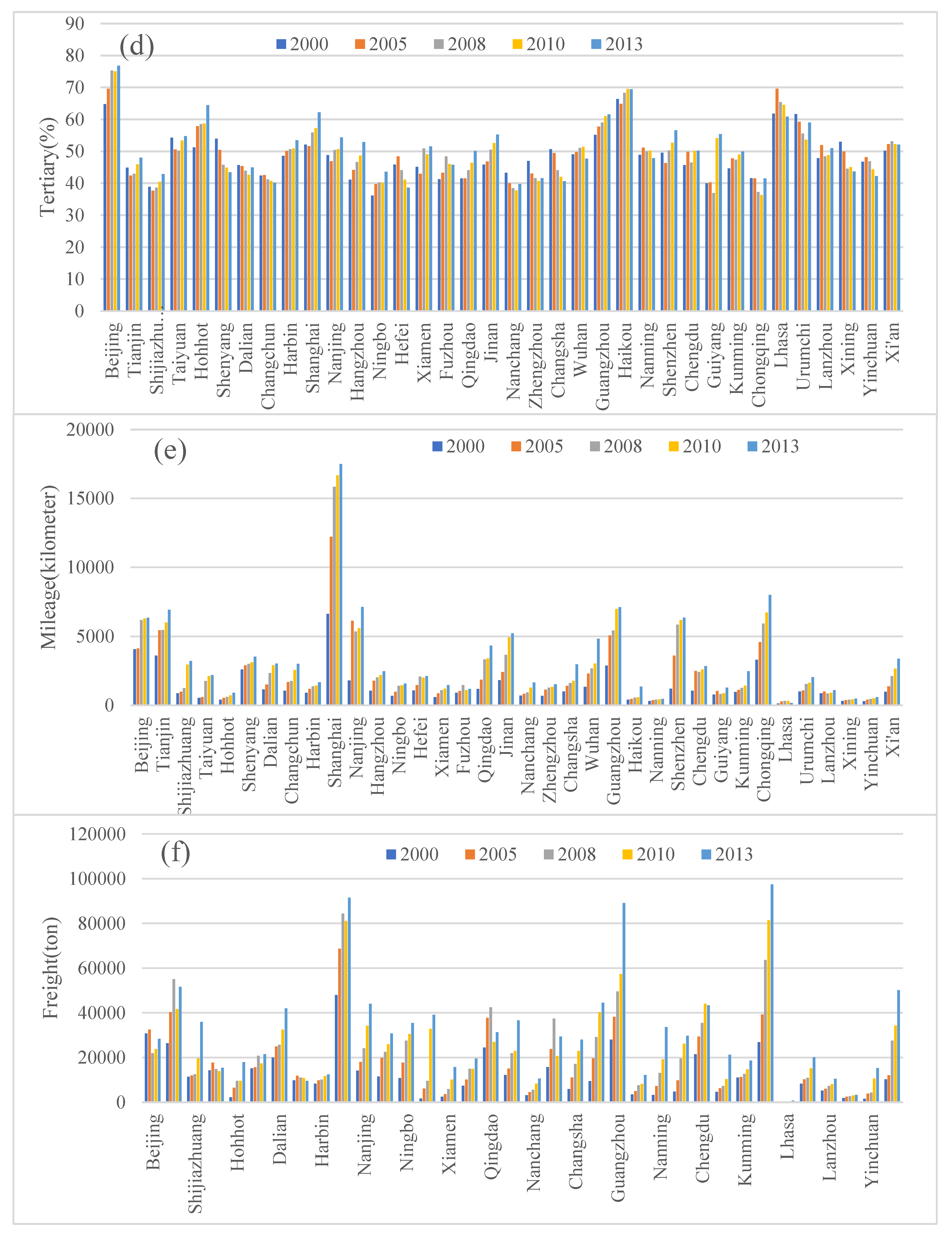
| Tertiary | The share of tertiary industry in GDP |
| Mileage | Mileage of paved roads (unit: kilometer) |
| Freight | The total volume of freight transport, including wheel transport, shipment, and airlift (unit: ton) |
| Coefficient | Estimate | Standard Error | t | p-Value |
|---|---|---|---|---|
| Intercept | −0.090 | 0.070 | −1.284 | 0.201 |
| GDP | 0.351 | 0.049 | 7.179 | <0.05 |
| POP | 0.416 | 0.098 | 4.230 | <0.05 |
| Secondary | 0.207 | 0.065 | 3.192 | <0.05 |
| Tertiary | 0.125 | 0.066 | 1.885 | 0.061 |
| Mileage | −0.009 | 0.074 | −0.120 | 0.904 |
| Freight | −0.020 | 0.042 | −0.483 | 0.630 |
| Summary statistics | ||||
| R2 = 0.728, Adjusted R2 = 0.718, F (6,173) = 77.053, p < 0.05 | ||||
| Coefficient | Estimate | Standard Error | t | p |
|---|---|---|---|---|
| Intercept | 4.044 | 0.062 | 65.121 | <0.05 |
| GDP | 0.642 | 0.117 | 5.464 | <0.05 |
| POP | 0.448 | 0.162 | 2.769 | <0.05 |
| Secondary | 0.544 | 0.103 | 5.274 | <0.05 |
| Tertiary | −0.482 | 0.110 | −4.375 | <0.05 |
| Freight | 0.134 | 0.107 | 1.259 | 0.210 |
| Mileage | 0.213 | 0.131 | 1.627 | 0.106 |
| Developed | 1.760 | 0.140 | 12.608 | <0.05 |
| Summary statistics | ||||
| R2 = 0.927, Adjusted R2 = 0.924, F (7,172) = 313.222, p < 0.05 | ||||
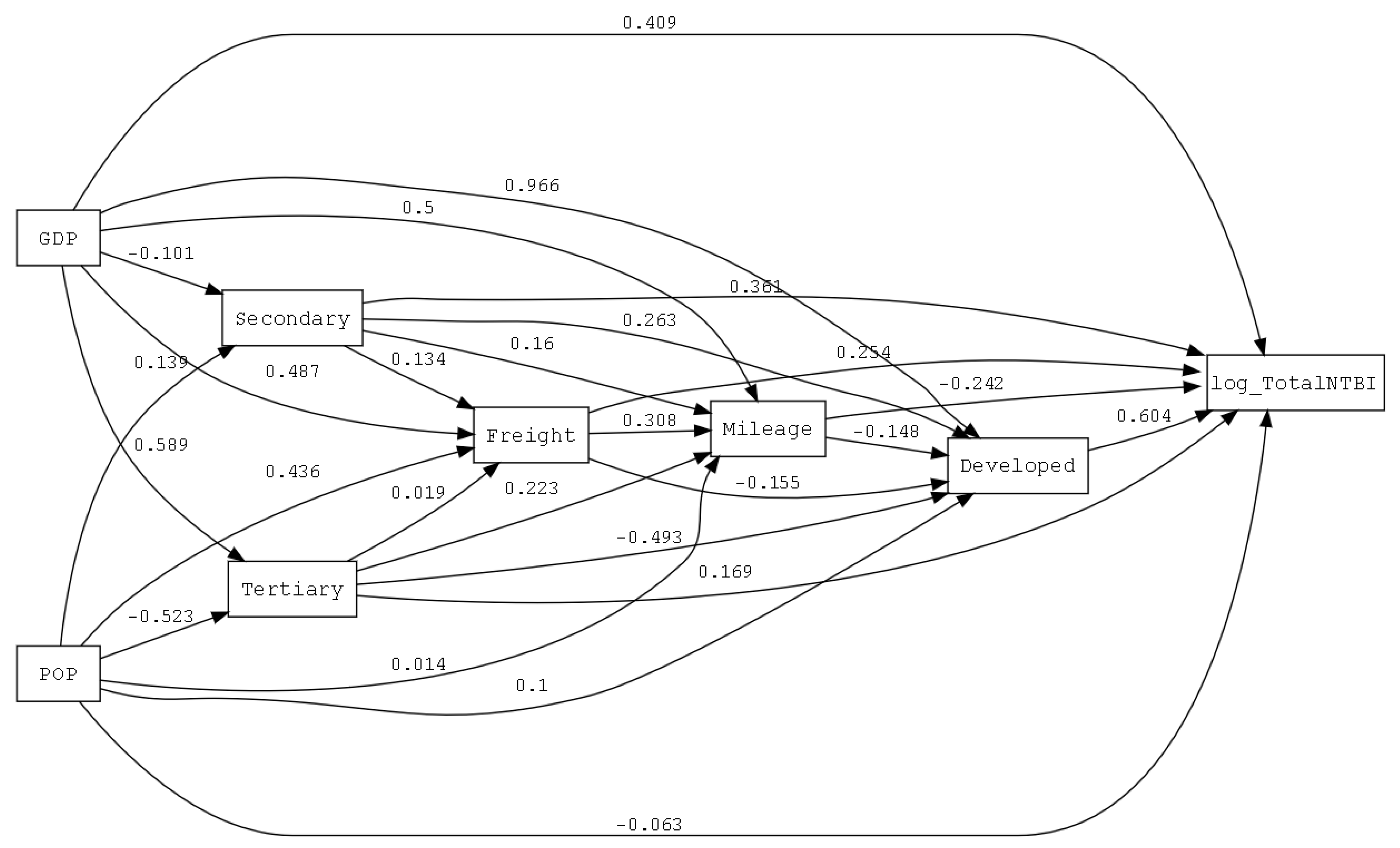
| Independent Variable | Developed | TotalNTBI | ||||
|---|---|---|---|---|---|---|
| Direct Coefficient | Indirect Coefficient | Total Coefficient | Direct Coefficient | Indirect Coefficient | Total Coefficient | |
| GDP | 0.966 | −0.416 | 0.550 | 0.409 | 0.351 | 0.760 |
| POP | 0.100 | 0.238 | 0.338 | 0.07 | 0.256 | 0.263 |
| Secondary | 0.263 | −0.027 | 0.236 | 0.361 | −0.213 | 0.148 |
| Tertiary | −0.493 | 0.033 | −0.460 | 0.169 | 0.026 | 0.195 |
| Mileage | −0.155 | −0.046 | −0.201 | 0.254 | −0.196 | 0.058 |
| Freight | −0.148 | 0.000 | −0.148 | −0.242 | −0.089 | −0.331 |
| Developed | - | - | - | 0.604 | 0.000 | 0.604 |
| Summary statistics X2 = 100.616, df = 3, p < 0.01 | ||||||
© 2018 by the authors. Licensee MDPI, Basel, Switzerland. This article is an open access article distributed under the terms and conditions of the Creative Commons Attribution (CC BY) license (http://creativecommons.org/licenses/by/4.0/).
Share and Cite
Li, H.-m.; Li, X.-g.; Yang, X.-y.; Zhang, H. Analyzing the Relationship between Developed Land Area and Nighttime Light Emissions of 36 Chinese Cities. Remote Sens. 2019, 11, 10. https://doi.org/10.3390/rs11010010
Li H-m, Li X-g, Yang X-y, Zhang H. Analyzing the Relationship between Developed Land Area and Nighttime Light Emissions of 36 Chinese Cities. Remote Sensing. 2019; 11(1):10. https://doi.org/10.3390/rs11010010
Chicago/Turabian StyleLi, Hui-min, Xiao-gang Li, Xiao-ying Yang, and Hao Zhang. 2019. "Analyzing the Relationship between Developed Land Area and Nighttime Light Emissions of 36 Chinese Cities" Remote Sensing 11, no. 1: 10. https://doi.org/10.3390/rs11010010
APA StyleLi, H.-m., Li, X.-g., Yang, X.-y., & Zhang, H. (2019). Analyzing the Relationship between Developed Land Area and Nighttime Light Emissions of 36 Chinese Cities. Remote Sensing, 11(1), 10. https://doi.org/10.3390/rs11010010