Differing Responses to Rainfall Suggest More Than One Functional Type of Grassland in South Africa

Abstract

Grasslands, which represent around 40% of the terrestrial area, are mostly located in arid and semi-arid zones. Semiarid ecosystems in Africa have been identified as being particularly vulnerable to the impacts of increased human pressure on land, as well as enhanced climate variability. Grasslands are indeed very responsive to variations in precipitation. This study evaluates the sensitivity of the grassland ecosystem to precipitation variability in space and time, by identifying the factors controlling this response, based on monthly precipitation data from Climate Hazards Group InfraRed Precipitation with Station data (CHIRPS) and the Fraction of Absorbed Photosynthetically Active Radiation (FAPAR) data from the Multi-angle Imaging SpectroRadiometer-High Resolution (MISR-HR) datasets, used as proxy for productivity, at 60 grassland sites in South Africa. Our results show that MISR-HR products adequately capture the spatial and temporal variability in productivity at scales that are relevant to this study, and they are therefore a good tool to study climate change impacts on ecosystem at small spatial scales over large spatial and temporal domains. We show that combining several determinants and accounting for legacies improves our ability to understand patterns, identify areas of vulnerability, and predict the future of grassland productivity. Mean annual precipitation is a good predictor of mean grassland productivity. The grasslands with a mean annual rainfall above about 530 mm have a different functional response to those receiving less than that amount of rain, on average. On the more arid and less fertile soils, large inter-annual variability reduces productivity. Our study suggests that grasslands on the more marginal soils are the most vulnerable to climate change.

1. Introduction

Grasslands, which are defined as ground covered with graminaceous plants with less than 10% tree and shrub cover [1], representing 40.5% of the global terrestrial area, excluding Greenland and Antarctica [2]. Extensive grasslands are mostly located in arid and semi-arid zones. Fires and herbivores are the two main biomass consumers of these grasslands, and these are fundamental to their ecology [3]. The livestock that supply meat, milk, leather, and fiber are mostly raised on grasslands [4]. Grasslands have a key role in greenhouse gas mitigation, in terms of carbon storage and sequestration [4].

Around a quarter of the grasslands globally are considered to be degraded [5,6,7]. Increased grazing intensity is among the key drivers of grassland degradation. In Africa and elsewhere, land degradation severity, extent, and trend depend on the nature of the soil, the agro-ecological zone, and the exploitation intensity of the natural resources by people and their domestic livestock [8]. Land degradation may be defined as the long-term, persistent loss of ecosystem function and capacity to generate ecosystem services. Some definitions also include the loss of grassland biodiversity [7]. In general, degradation is considered to be human-induced, either directly or indirectly; for instance, through climate change. In grasslands, it is the result of a combination of processes such as soil erosion, the deterioration of desirable soil properties, loss of natural vegetation cover, a switch to a plant species community (either indigenous or alien) that is less desirable than the native community, or an ecohydrological change resulting in poorer infiltration of rainfall [9]. The key ‘ecosystem function’ that implicitly underpins most of these definitions is the net primary productivity (NPP) [10,11]. A standard or benchmark for grassland productivity is required to detect a ‘persistent reduction’ in NPP, and several studies identify the absence of a quantitative benchmark of expected vegetation status as an impediment to detecting degradation in grasslands [12,13]. In the absence of a benchmark, a decline in NPP can be inferred from a long production time series, provided that the degradation occurs in the observed period. These two conditions are seldom met; thus, an accurate model of what the expected productivity would be under given circumstances would provide a useful reference level.

In parallel with an increased use-pressure on the land, projections of climate change suggest that many drylands, including in southern Africa, will face increased rainfall variability, often associated with decreased soil moisture resulting from one or both of decreased average rainfall or increased evaporative demand. The increase variability leads to an increased frequency of extreme events, such as floods or drought [14]. Drylands, comprising arid, semiarid, and dry sub-humid ecosystems, are characterized by having water-limitations to plant growth for a large part of the year—more than three months continuously, but typically six months or more [15]. Semiarid ecosystems in Africa have been identified as being particularly vulnerable to the impacts of warming, drying, and increased climate variability [16]. Biome comparisons indicate that grasslands are more responsive, in the short term, to variation in precipitation than are most ecosystems. Precipitation is the key factor in controlling the primary productivity of most of the world’s grassland ecosystems, and by definition, this is especially so for arid and semi-arid regions [17,18,19]. Plant growth is limited by water availability, which reflects a balance between inputs (rainfall) and losses (evaporation from the soil, transpiration and drainage), mediated by storage in the soil profile. Since evaporative demand is much less variable than rainfall between years and places—and in semi-arid grasslands it is typically two to three times in excess of rainfall—low and variable precipitation is the key proxy for plant water availability.

A large fraction of the variability in grassland productivity can be explained by precipitation variability, and to some extent, local soil characteristics [20,21,22]. The correlation between productivity and precipitation is stronger across space than through time [23]. In the range of 400 to 800 mm of Mean Annual Precipitation (MAP), the spatial variability in the mean annual aboveground grassland productivity (AGNPP) is well-predicted by a simple linear regression model; and essentially the same relation holds across several continents, including southern Africa. This relation, AGNPP (gDM m⁻² y⁻¹) ≌ 0.58 MAP (mm), accounts for 80% or more of the spatial variability.

For a single site, on the other hand, the year-to-year variation in precipitation accounts, on average, for only 15% of the inter-annual variability in grassland productivity (the range is 0% to 77%). Some studies suggested that the lower correlation through time than space is a result of the interaction between nutrients and water to limit or boost growth in particular years [24], while others hypothesize that it may be due to legacy effects based on drought or abundance in previous years, i.e., a multi-year lag in the response of ecosystems to changes in water availability [23,25,26]. Few studies have combined both environmental and legacy effects to identify areas of vulnerabilities of semi-arid grasslands to climate change. From the perspective of climate change, ‘vulnerability’ refers to the probability of some desirable property—in this case AGNPP—being negatively affected by the change in the mean climate or its variability (including extreme events). A better understanding of the sensitivity of grassland productivity to climate mean and variability is a key step to assessing their vulnerability.

The objective of this study was to assess the sensitivity of the semi-arid grassland ecosystems of southern Africa to mean rainfall and its inter-annual variability. The following research questions were formulated:

• How sensitive is the productivity of grasslands in semi-arid regions to mean rainfall and inter-annual variability?
• Which factors affect this sensitivity, and what is the role of legacy effects?
• What factors differentiate or correlate the sensitivity of these ecosystems to average precipitation and inter-annual variability?
• What are the implications of grassland sensitivity for their vulnerability under future climates?

The sensitivity was evaluated at 60 representative natural grassland sites within South Africa, using a 15-year multi-temporal record of Multi-angle Imaging SpectroRadiometer-High Resolution (MISR-HR) satellite data [27]. The sites selection process is described in Section 2.2.1. Monthly values of the Fraction of Absorbed Photosynthetically Active Radiation (FAPAR) were extracted at a 275 m spatial resolution, over the entire grassland domain. FAPAR is a good indicator for vegetation productivity [28], since it is physically-based and directly linked to the carbon assimilation process. The FAPAR product derived from satellite-based sensors such as MISR constitutes a spatially and temporally consistent long-term dataset. Monthly rainfall was obtained from the Climate Hazards Group InfraRed Precipitation with Station data (CHIRPS) dataset [29], at an approximately 5 km spatial resolution.

The paper is organized as follows. In Section 2, the datasets and the method of analysis are introduced. Section 3 shows results, which are discussed in Section 4; and conclusions are drawn in Section 5.

2. Materials and Methods

2.1. Datasets

The following datasets were used:

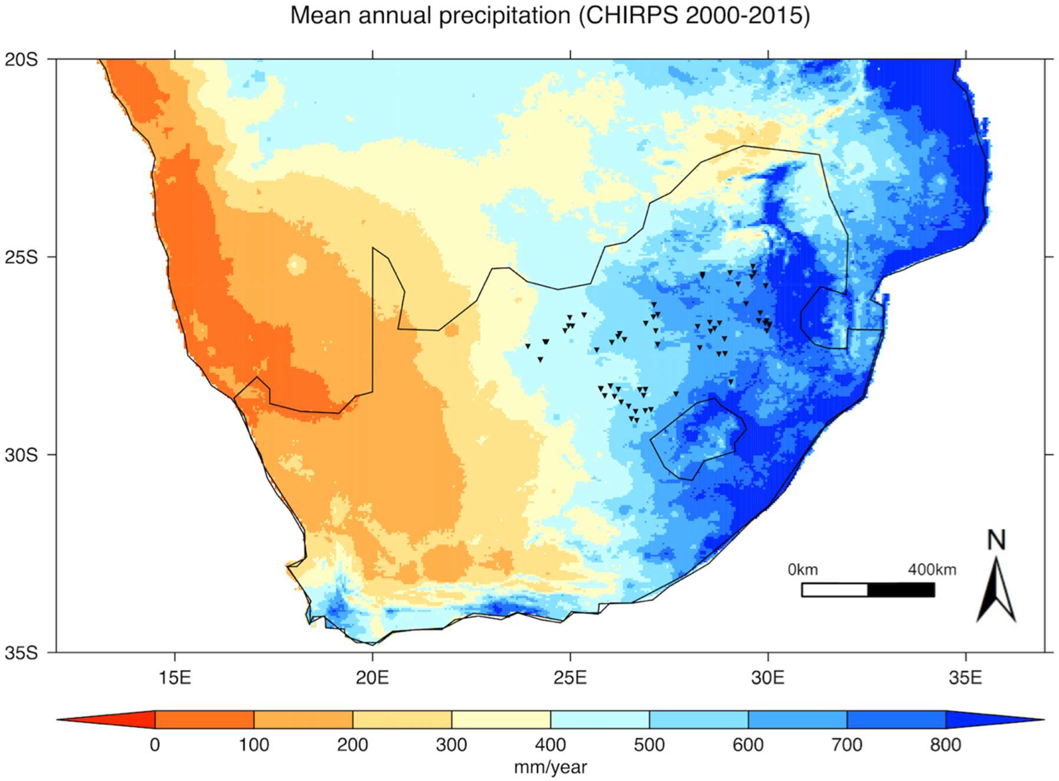
• Monthly precipitation data were extracted from the Climate Hazards Group InfraRed Precipitation with Station data, CHIRPS v2.0 [29], which covers the latitude band 50°S–50°N at all longitudes, from 1981 to the near-present, at a 0.05° spatial resolution (available from http://chg.geog.ucsb.edu/data/index.html). This dataset incorporates monthly precipitation climatology from the Climate Hazards Group’s Precipitation Climatology version 1 (CHPClim), infrared satellite observations from the Climate Prediction Center (CPC) and the National Climate Data Center (NCDC), the Tropical Rainfall Measuring Mission (TRMM) product, atmospheric model rainfall fields from the Coupled Forecast System version 2 (CFSv2), and in situ precipitation observations obtained from a variety of sources including national and regional meteorological services. The relevance and applicability of this dataset for this study were evaluated by comparing it to precipitation records independently provided by the South African Weather Service for five weather stations located within the study area (Bloemfontein, Vryburg, Potchefstroom, Johannesburg and Witbank).
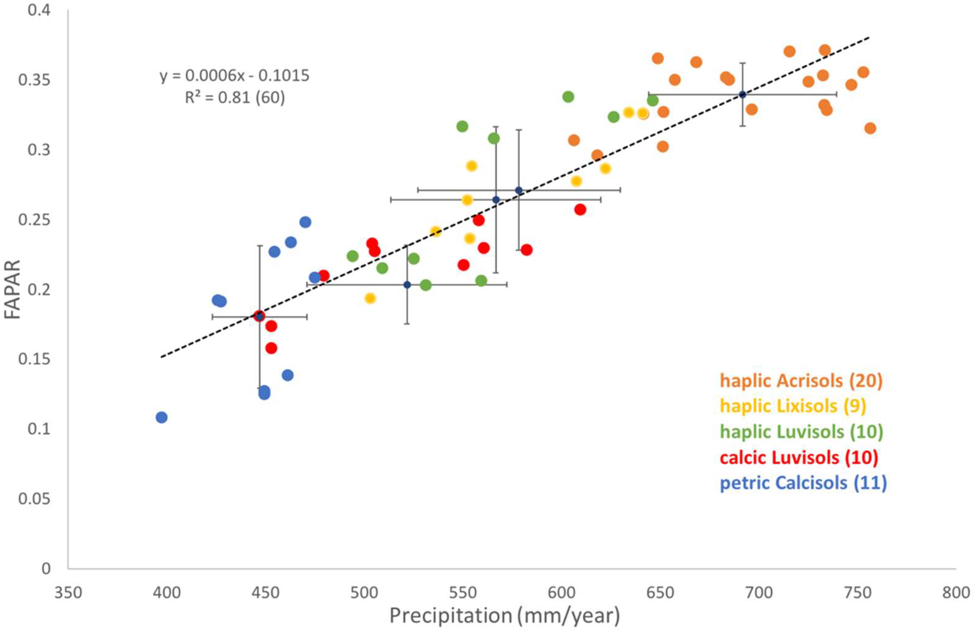
• The seasonally-accumulated FAPAR, estimated from the high resolution MISR-HR satellite product [27], were used as a proxy for grassland productivity. These FAPAR data, at a spatial resolution of 275 m, have been available since late February 2000 from the Global Change Institute, University of the Witwatersrand (free on request to [email protected]). The product is delivered in the Space Oblique Mercator projection format. The repeat frequency of observation of an arbitrary site (under identical observation geometries) is 16 days. However, due to the overlap of successive paths and the fact that any site in South Africa can be observed from three such paths, the revisit frequency is much higher, at around six times per month. This feature partially mitigates the problem of missing data due to cloud cover, especially during the rainy season.
• Natural grassland areas (i.e., excluding croplands, abandoned fields, plantations and other land uses within the grassland biome) were extracted from the 30 × 30 m 2013–2014 South African National Land-Cover Dataset [30] which was derived from an analysis of the 2013–2014 Landsat 8 satellite imagery. This data can be found at http://bgis.sanbi.org/DEA_Landcover/project.asp. The potential grassland sites were further assessed against the “grassland” class of the 2010 global land cover map from the European Space Agency (ESA), available at a 300 m resolution based on MERIS [31], and the same class of the 2014 global land cover GLC map, available at a 1 km resolution based on global and national datasets [32]. These datasets can be downloaded respectively at https://www.esa-landcover-cci.org and at http://www.earthenv.org/landcover.
• Soil information for the selected grassland sites were acquired from the AfSoilGrids 25 dataset [33]. The dataset contains soil characteristics—including soil organic carbon (gC/kg), pH (in H₂O), fraction of sand (kg/kg), silt (kg/kg) and clay (kg/kg), bulk density (kg/m³), and cation-exchange capacity (CEC, cmol ⁺/kg), in addition to estimates of depth to the bedrock (cm), the probability of occurrence of R horizon or bedrock within 20 m, and the distribution of soil classes based on the World Reference Base (WRB) and the United States Department of Agriculture (USDA) classification systems—for the whole African continent at 25 spatial resolution at seven standard soil depths (0, 5, 15, 30, 60, 100, and 200 cm). This gridded dataset was derived using machine learning techniques from ca. 150,000 soil profiles and a stack of 158 soil covariates, mostly derived from the Moderate Resolution Imaging Spectroradiometer (MODIS) land products, Shuttle Radar Topography Mission (SRTM) digital elevation model (DEM) derivatives, spatially interpolated climate data on grids, and global landform and lithology maps. This dataset can be found at https://www.isric.online/projects/soil-property-maps-africa-250-m-resolution.
• Data on herbivory and fire were taken from Archibald et al. [3] who produced maps for sub-Saharan Africa at a resolution of 0.5° × 0.5° of the mean consumption of above ground NPP by fire and herbivory. These data were made available for this study by S. Archibald. The fire data are an aggregate of 50 resolution MODIS burned area data for the period from 2000 to 2015. There is no reliable source of high-resolution herbivory data; this product combines livestock census data with estimates of wildlife biomass.

2.2. Method

2.2.1. Grassland Sites and Selection

The 60 sites were selected to be representative of the entire grassland biome of South Africa; distributed over the MAP range of 400–80 m per year; and on a variety of soil types (Figure 1). The exact location of each site was determined using an individual visual assessment of high-resolution imagery to be homogeneous, in un-degraded natural grassland, and large enough (radius 1 km) to allow for the resolution and pointing accuracy of the instrument. The sites are selected in such a way that they are well spread over the selected precipitation range and soil type classes. The description of the five different World Reference Base (WRB) soil classes represented (petric Calcisols, haplic Luvisols, calcic Luvisols, haplic Lixisols, haplic Acrisols) is provided in Appendix A.

2.2.2. Data Preparation

MISR-HR FAPAR products were extracted from the Global Change Institute (GCI) database and aggregated into monthly averages as follows: Let i be the index pointing to one of the I = 60 sites, and let t be the index of the calendar month of interest within the nominal set of T = 180 months available at the start of this investigation (15 years, from 2000 to 2014, of 12 months). The NASA Terra platform hosting the MISR instrument is on a repeating trajectory, such that the instrument observes the same locations on the planet from the same direction every 16 days (233 orbits), or twice a month. These patterns of repeating orbits are called paths, and the latitude-dependent overlap between spatially contiguous MISR paths is such that each site in South Africa is actually observable from three separate paths, hence six times per month. At each site, and for each available orbit on the three relevant paths, the FAPAR product were extracted over a small square window of 3 by 3 MISR-HR pixels, centered on the site’s nominal geographical location. Let l be the index pointing to these individual pixel values: l = 1, 2, …, L, where L = 9. If m is the number of available paths (0 ≤ m ≤ M), with M = 3, and if n_m is the number of available orbits on path m (0 ≤ n_m ≤ N_m), with N_m = 2, the maximum number of FAPAR samples (individual pixel values) that could be retrieved for a site in a calendar month is thus K = 9 × 3 × 2 = 54.

The actual number of usable measurements will be smaller, however, because of the frequent presence of clouds that prevent surface measurements, especially during the rainy season, or occasional missing observations due to technical issues. Let then λ be the actual number of effectively available pixel values in a particular square window acquisition (0 ≤ l ≤ λ ≤ L) for a specific orbit, let μ be the actual number of effectively available MISR paths for the specified site (0 ≤ m ≤ μ ≤ M), and let ν_m be the actual number of effectively available MISR orbits for that path m (0 ≤ n ≤ ν_m ≤ N_m). The monthly average FAPAR value for site i and month t was then estimated as:

$$\overline{FAPAR\left(i,t\right)}=\frac{1}{\lambda \mu \nu }{\sum }_{l=1}^{\lambda }{\sum }_{m=1}^{\mu }{\sum }_{n=1}^{\nu }FAPAR\left(l,m,n\right),$$

(1)

FAPAR(i,t) is an estimate of the mean FAPAR value at site i during month t. In the case that FAPAR(i,t) could not be computed, for example due to cloud cover, its value was interpolated, but only if at most two consecutive monthly values were missing. This approach is appropriate because a regression analysis showed that FAPAR values for the current month were highly correlated to those for the previous month. The missing value FAPAR(i,t) was estimated as the average of two predictors. The first one $\overline{FAPA{R}_1\left(i,t\right)}$ is the average value of all available monthly values for the particular month of the year, and the second $\overline{FAPA{R}_2\left(i,t\right)}$ is the average of the preceding and successive values within the same year.

Formally, these were computed as follows: Let τ* denote the number of effectively available monthly values for the missing month of the year, within the T* = 15 years of record (from 2000 to 2014), and let t* be the index within that set (0 ≤ t* ≤ τ* ≤ T*). Then:

$$\overline{FAPA{R}_1\left(i,t\right)}=\frac{1}{\tau \ast }{\sum }_{t^{\ast }=1}^{{\tau }^{\ast }}FAPAR\left(i,t^{\ast }\right),$$

(2)

where the starred indices refer to values associated with the particular month of the year. The equation to estimate the second predictor depends on whether the missing value is surrounded by valid values, or whether there are two consecutive missing values (no interpolation was attempted if there are more than two consecutive missing values). For an isolated missing value:

$$\overline{FAPA{R}_2\left(i,t\right)}=\frac{1}{2}\left[FAPAR\left(i,t-1\right)+FAPAR\left(i,t+1\right)\right],$$

(3)

and if there are two consecutive missing values, the first one was estimated as:

$$\overline{FAPA{R}_2\left(i,t\right)}=\frac{2}{3}\left[FAPAR\left(i,t-1\right)+\frac{1}{3}FAPAR\left(i,t+2\right)\right],$$

(4)

and:

$$\overline{FAPA{R}_2\left(i,t+1\right)}=\frac{1}{3}\left[FAPAR\left(i,t-1\right)+\frac{2}{3}FAPAR\left(i,t+2\right)\right],$$

(5)

respectively, where t in the last two equations points to the first missing month. The missing value was then computed as:

$$FAPAR\left(i,t\right)=\frac{1}{2}\left[\overline{FAPA{R}_1}+\overline{FAPA{R}_2}\right],$$

(6)

This guarantees that the replacement values do not steer too far away from the long-term mean for that month, but they are also allowed to represent conditions that may be particular during that year.

Next, for each grassland site, the monthly rainfall data for the CHIRPS grid cell that covers the site were retrieved. For both the monthly FAPAR and precipitation datasets, the yearly cumulative values between July and June of the following year were computed over the 2000–2014 period, given that the growing season typically extends from October to April. The same procedure was performed for the CHIRPS grid cells covering the five weather stations for which the yearly precipitation data were provided by the South African Weather Service (SAWS). The correlation between CHIRPS and the weather stations precipitation was found to be significant (Figure A1 in Appendix B, CHIRPS = 0.62SAWS + 220; R² = 0.74, n = 75). Since the study is correlative, the CHIRPS precipitation dataset was considered to be an appropriate proxy for site rainfall for this study.

Finally, for each of the 60 sites, a 3 × 3 matrix of AfSoilGrids25 pixels at each site was selected. The average values of the different soil characteristics over these nine pixels were computed by soil depth class. For the WRB soil class, which is not a quantitative variable, the most frequent soil class over the nine pixels was assigned to the site. For fire and herbivory, the grid cells that cover the different sites were retrieved from the database developed by Archibald et al. (2016) [3].

2.2.3. Data Analysis

First, the spatial variability of mean annual grassland productivity was examined. The potential factors that might affect this variability were estimated based on the analysis of the spatial correlations between the multi-year mean FAPAR, the mean precipitation, the range of precipitation inter-annual variability (defined as the inter-annual standard deviation), the nine quantitative soil characteristics, and the consumption by fire and herbivory, over the period 2000–2014 and for all sites. The Pearson correlation coefficient was used to characterize the strengths of the relations between the multi-year mean FAPAR and the 13 site-specific variables mentioned above, and to rank those variables in order of decreasing importance in explaining the spatial variability in grassland productivity. The significance level of a correlation was arbitrarily set at p = 0.1. The linearity of the relations between those variables was assumed. Based on the results of this correlation analysis, further analyses were performed, with the soil depth showing the overall best correlation between soil characteristics and multi-year mean FAPAR.

The slope of the regression between multi-year mean FAPAR and the mean precipitation at each site was used as a proxy for the sensitivity of grassland productivity to spatial variation in precipitation. To assess the potential factors affecting the response of grassland productivity to spatial variation in precipitation, multivariate linear models were constructed, using the least square method, with the multi-year mean FAPAR as a response variable and the multi-year mean precipitation plus one, two, three… up to 12 of the other site-specific variables as explanatory variables. From this set of 12 models, the best one was selected based on the Akaike Information Criterion (AIC) [34]. AIC is a model selection criterion that penalizes models, in which adding new explanatory variables does not supply additional information to the model, the information being measured by the mean squared error. The AIC works to balance the complexity of a given model and its goodness-of-fit.

Next, the sensitivity of annual grassland productivity at each site to the inter-annual rainfall variability at that site was assessed. To evaluate the period of the year during which precipitation had the most significant impact on seasonally-accumulated productivity, lagged correlations were performed over the 2000–2014 period at each site between the time series of the yearly FAPAR and the time series of precipitation cumulated over different time windows. The time windows considered were 1, 3, 6, and 12 months in length, starting from every month one year prior to the start, until the end of current growing season. The sensitivity of the annual productivity to the inter-annual variability of the rainfall within those different time windows was estimated at each site, based on the slope of the regression through annual FAPAR, and the precipitation within the time windows. The Pearson coefficient was again used to assess the strength of the correlation between datasets.

To estimate the factors affecting the sensitivity of annual productivity to precipitation inter-annual variability, the spatial variation in correlation strength between those different temporal correlations was evaluated against the spatial variation in precipitation, mean, and range in inter-annual variability, soil characteristics, and consumption by fire and herbivory at each site, in a similar way, as described above for the spatial variability in multi-year FAPAR and the various site-specific variables. The point in time during the growing season when the monthly productivity becomes a significant proxy for the annual productivity was estimated based on the strength of the correlations between the time series of the yearly FAPAR and the time series of the monthly FAPAR values of each month of the year. Here as well, the factors affecting the strength of the correlations were evaluated.

Finally, we evaluated the legacy effects on grassland productivity and the impact of abnormally wet and dry years. At each site, the annual FAPAR anomalies were computed, by subtracting the multi-year mean FAPAR from the annual means, and normalized by the multi-year mean FAPAR. Normalized cumulative precipitation anomalies were computed as well, over the four time windows mentioned above; i.e., 1, 3, 6, and 12 months. Based on these normalized FAPAR and precipitation anomalies, contingency tables were produced and evaluated with respect to 13 site-specific variables: the precipitation mean and inter-annual variability, the nine soil characteristics, herbivory, and fire, as well as with the precipitation anomalies during the previous growing season. These tables helped to isolate the nature of the precipitation event that favor extreme or unusual FAPAR anomalies, as well as the site-specific characteristic that tends to enhance or inhibit this behavior.

3. Results

3.1. Spatial Variability in Grassland Productivity

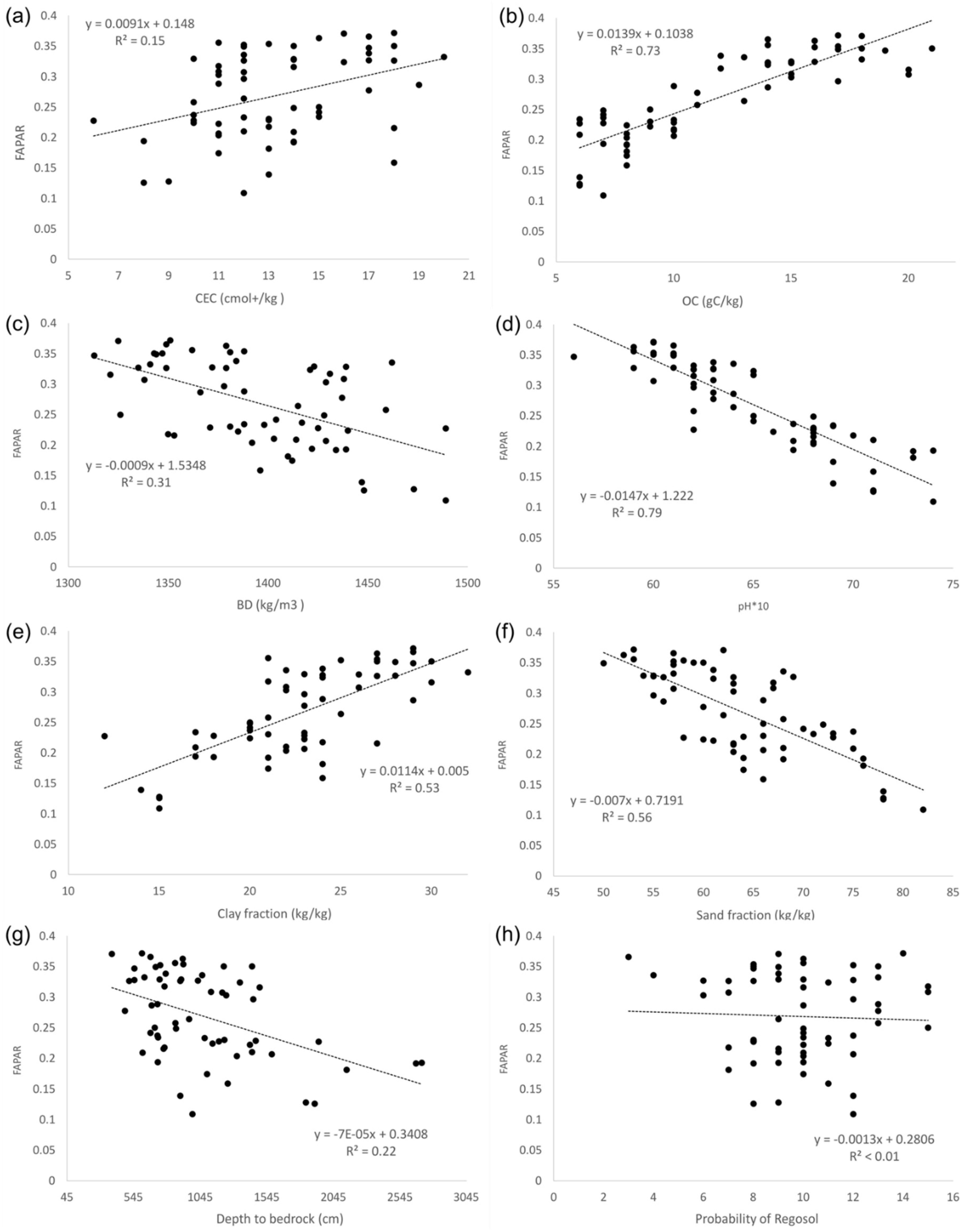
3.1.1. Factors Affecting Spatial Variability in Productivity

The correlation between the multi-year mean FAPAR values and the multi-year MAP at the grassland sites is highly significant, and it accounts for a large fraction of the FAPAR spatial variability (R² = 0.81). Figure 2 shows that different soil type classes are successively encountered along the precipitation gradient; i.e., the soil type evolves through the sequence petric Calcisols, calcic Luvisols, haplic Luvisols, and Lixisols and haplic Acrisols, as MAP increases from 400 to 800 mm y⁻¹. As a result, each of the soil classes exhibited a significantly different range of MAP and mean FAPAR, except the haplic Lixisols and Luvisols (see standard deviation in Figure 2). Thus, soil properties are conflated with rainfall, which hampers further investigation of the effects of soil texture on the relationship, since the wetter locations tend also to have lower pH, more clay, and more organic matter.

The multiyear FAPAR at the different sites is significantly (p-value < 0.1) correlated to all soil variables, except to the probability of occurrence within 20 m of the surface of a R horizon (hard bedrock) (see Figure A2 in Appendix C). All soil correlations are based on the values for soil properties at m soil depth, because overall the correlation between FAPAR and soil properties was greatest at that depth. More than half of the spatial variability in FAPAR can be explained by the spatial variability of one of the following individual soil variables (note that for n = 60, any R² above around 0.15 is statistically significant at the 90% confidence level): soil pH (R² = 0.79), soil organic carbon content (R² = 0.73), and soil texture; i.e., sand (R² = 0.56) and clay (R² = 0.53) content. The FAPAR tends to increase with decreasing pH and sand fraction, and with increasing soil organic content and clay. The soil pH values of the 60 sites lie between 5.7 and 7.5. Those four soil variables are all correlated with the MAP, and with each other; in particular, precipitation and soil pH are strongly negatively correlated. The FAPAR is also significantly positively correlated with CEC (R² = 0.15) and silt fraction (R² = 0.16), and negatively correlated with soil bulk density (R² = 0.31) and depth to bedrock (R² = 0.22). The correlation of FAPAR with grass consumption by fire and herbivory is positive and significant in both cases, but stronger in the case of fire (R² = 0.51) than with herbivory (R² = 0.18). Consumption by fire is also strongly correlated with the four soil characteristics mentioned above. The multi-year mean FAPAR is not significantly correlated to the precipitation inter-annual variability (p-value > 0.1) at the 60 grassland sites.

3.1.2. Sensitivity of Grassland Productivity to Spatial Variation in Precipitation

Figure 2 shows that the multi-year mean FAPAR increases by 6 × 10⁻⁴ for each mm increase in mean annual precipitation. To assess the factors affecting this sensitivity, 12 multivariate linear models were constructed, using as the dependent variable the multi-year mean FAPAR at the 60 sites, and as explanatory variables the multi-year mean precipitation and one to 12 of the site-specific variables discussed above, including inter-annual rainfall variability. Based on the AIC, a four-variable model was selected (see

Table A1. Summary table of the variables selected, based on the least square method, for each multivariate linear model with the multi-year mean FAPAR as the response variable and the multi-year mean precipitation plus one up to 12 other site-specific variables. The “best” model was selected based on the AIC.

Nbr. of variables	Variables	MSE	R²	Akaike’s AIC
1	Mean precip	0.001	0.805	412.225
2	st dev precip/Mean precip	0.001	0.851	−426.178
3	st dev precip/Mean precip/fire DMI	0.001	0.861	−428.381
4	st dev precip/Mean precip/BD/fire DMI	0.001	0.865	−428.411
5	st dev precip/Mean precip/BD/Clay/fire DMI	0.001	0.869	−428.250
6	st dev precip/Mean precip/BD/Clay/Depth to bedrock/fire DMI	0.001	0.872	−427.575
7	st dev precip/Mean precip/BD/Clay/Sand/Depth to bedrock/fire DMI	0.001	0.875	−426.858
……

The best model for the selected selection criterion is displayed in bold.

in Appendix D). The four variables are, in order of added value: multi-year mean rainfall, rainfall inter-annual variability; consumption by fire and soil bulk density. Collectively, they explain 87% of the spatial variability in multi-year mean FAPAR. The mean rainfall explains 81%, rainfall inter-annual variability a further 4%, and consumption by fire and the soil bulk density improve the model by 1% each. The rainfall variability and bulk density tend to reduce the sensitivity of grassland productivity to the precipitation spatial variability, while consumption by fire enhances it.

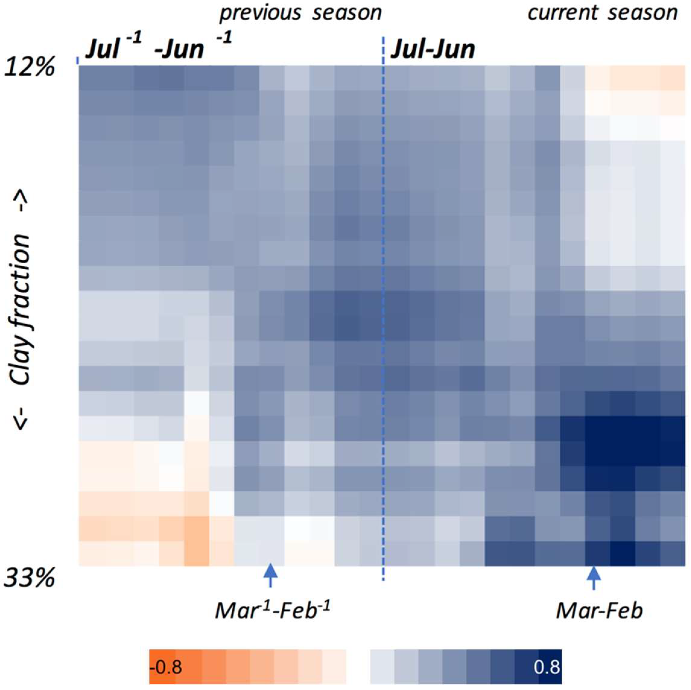
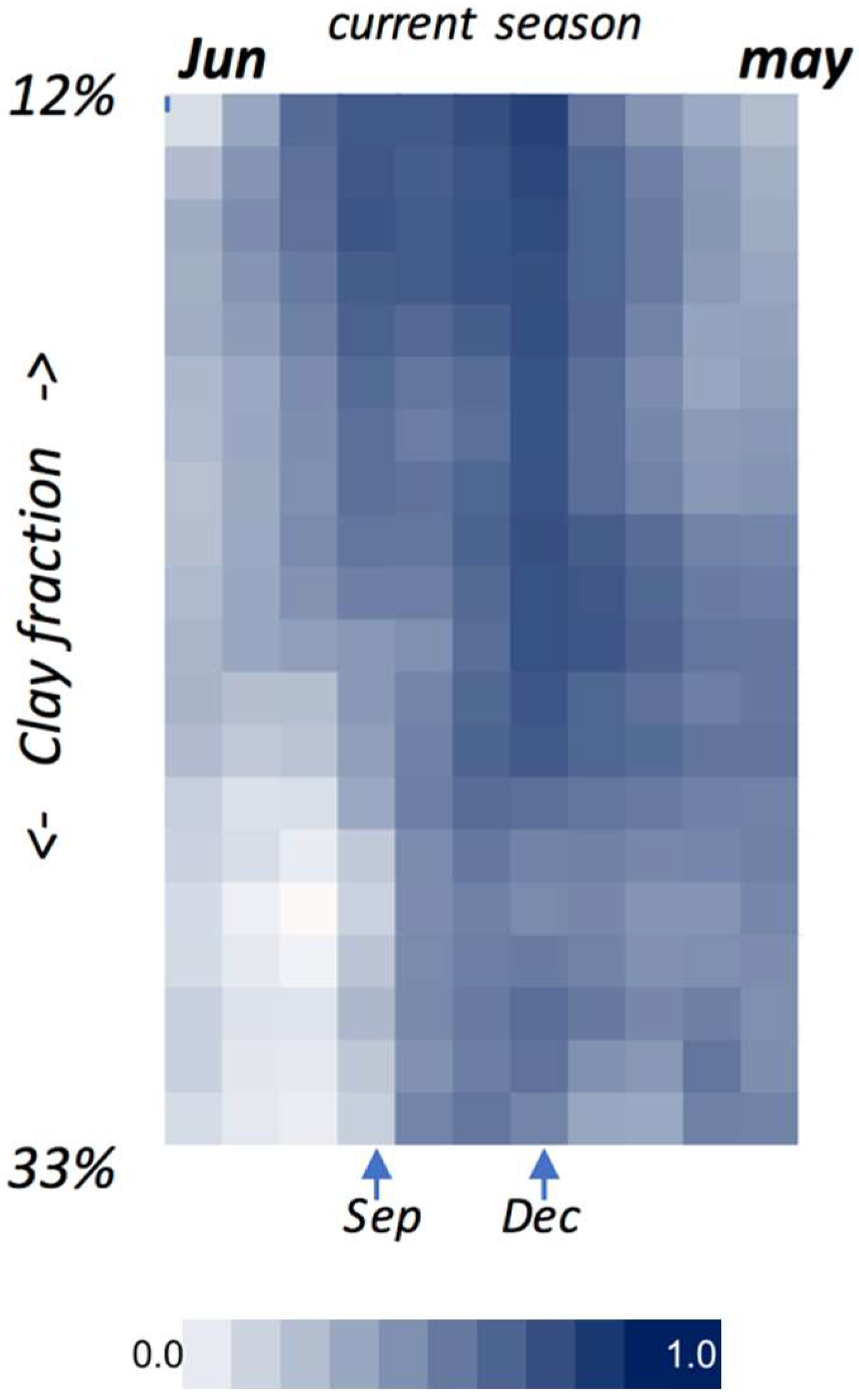
3.2. Temporal Variability in Grassland Productivity at a Site

3.2.1. Sensitivity to Rainfall and the Factors Affecting It

During the 2000–2014 period, positive correlations exist at all sites between the annual FAPAR values, and the precipitation over the four moving time windows within a season; i.e., the monthly cumulated precipitation for 1-, 3-, 6-, and 12-month, from one year prior to the start of the growing season until the end of the season. The strength of the correlations varies strongly between sites and over time. On average, the correlations are the strongest when the rainfall is accumulated over 12 months. Of the various site-specific variables, the clay fraction at m soil depth best explains the variability in correlation strength between sites and along time windows. Figure 3 shows a clear pattern in correlation strength: at sites on soils with a higher clay fraction, the amount of rainfall during the current (rather than previous) season explains more of the FAPAR inter-annual variability. With decreasing clay fraction, the current season precipitation becomes gradually less significant, while the effect of previous season precipitation grows, but never to the extent of dominating current season rainfall as a predictor. There seems to be a gradual shift of influence from the previous to current season precipitation with increasing soil clay content. Unsurprisingly, the rainfall during the drier winter months in between two growing seasons (April to August) hardly contributes to the yearly FAPAR of the current growing season. Nonetheless, the largest variability between sites in correlation strength is observed for the precipitation accumulated between March and the following February; in other words, the contribution of the end of the past growing season and the beginning and middle of the current growing season. Some 42% of the spatial variability in correlation strength between the current season FAPAR and the cumulated precipitation between March and February can be explained by the clay fraction in the soil.

The sensitivity of annual grassland productivity to precipitation inter-annual variability is revealed by the slope of the regression line at each site between the annual FAPAR and the accumulated precipitation. Sensitivity shows a similar pattern in relation to the various time windows, as did correlation strength in Figure 3. The maximum sensitivity FAPAR is about 3.6 × 10⁻⁴ FAPAR units for each mm of rainfall accumulated between March of the previous season and February of the current season, and it is encountered on clayey soils with high clay fraction. The intercept of the regression is strongly linked to the slope, and it tends to decrease with increasing clay content.

3.2.2. Relationship with in-Season Grassland Productivity

Figure 4 shows a contingency table of the correlation strength between the yearly FAPAR and the monthly FAPAR values between the start and the end of the growing season. From this figure, it can be seen that on soils with low clay fractions, the FAPAR observed in August–September already significantly correlates to the yearly-accumulated FAPAR. On those soils, the values of the Pearson coefficient increase from June to December, and gradually decrease thereafter. With increasing clay fraction, the point in time during the growing season when the correlation becomes significant gradually shifts to a later date; i.e., October–November. Hereafter, the strength of the correlations fluctuates but tends to remain lower than on less clayey soils.

Multivariate linear models were constructed using the Pearson coefficients of the regression between annual and monthly FAPAR at each site as the dependent variable, and from one to 13 site-specific variables as the explanatory variables. For each month, the best models were selected based on the least square method and the AIC. Clay fraction and consumption by herbivory were in general the most significant variables, and they collectively explained 54% and 45% of the spatial variability in the Pearson coefficient values for the months of September and December respectively. From all available explanatory variables, the clay fraction at m depth was here again the best predictor, explaining 47% of the spatial variability in September and 34% in December.

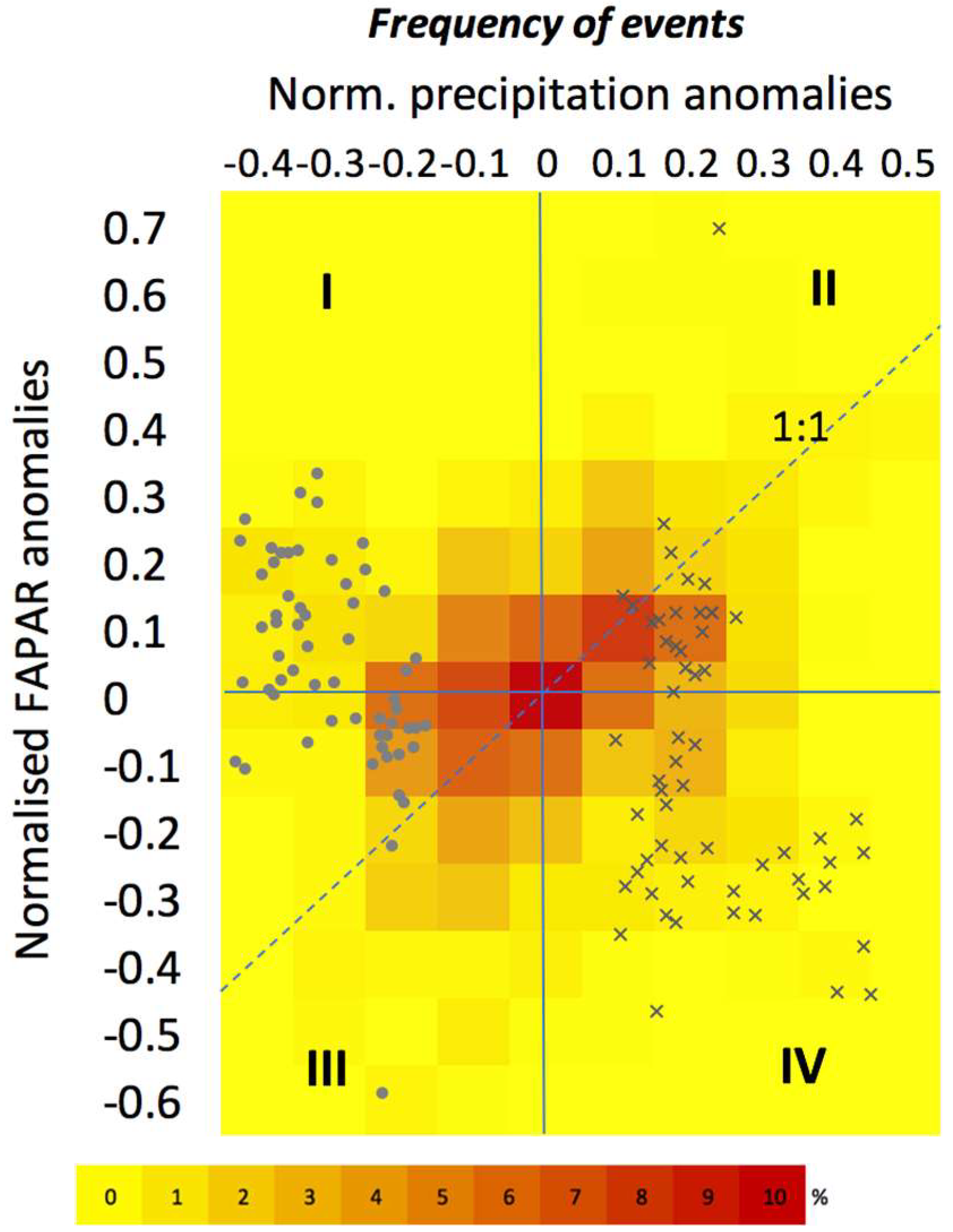
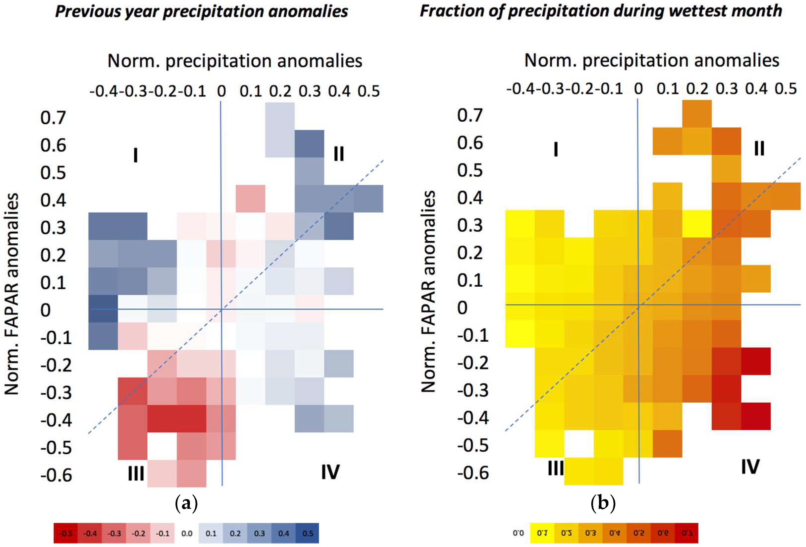
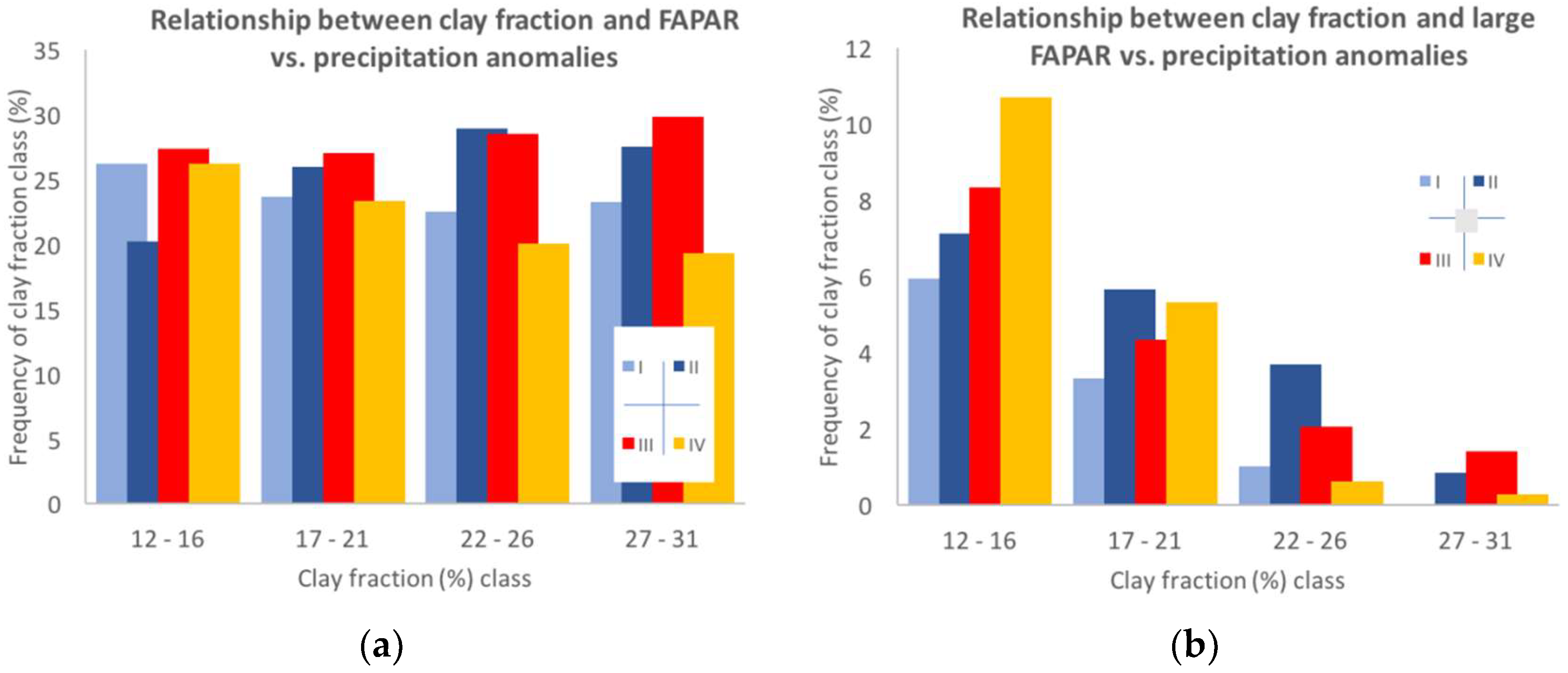
3.3. The Impact of Extreme Precipitation Events

3.3.1. Nature of Precipitation Event

Positive and negative annual precipitation anomalies tended to result in positive and negative FAPAR anomalies (Figure 5). However, some of the FAPAR anomalies exhibited a different relation, not clustered around the 1:1 line in Figure 5. For instance, the summer of 2008–2009 were much wetter than usual (rainfall was two standard deviations above the mean), but only a small subset of sites showed a positive FAPAR deviation from the long-term mean; and many sites exhibited a lower yearly FAPAR than the long-term average for that year (quadrant IV in Figure 5). Similarly, the summer of 2010–2011 rainfall was two standard deviations below the mean, but most sites were characterized by a larger yearly FAPAR value than average (quadrant I in Figure 5).

Figure 6a shows that years with negative precipitation anomalies but positive FAPAR anomalies were preceded by very wet years (quadrant I in Figure 6a), and they are markedly clustered above the 1:1 line. Years with medium-to-high positive rainfall anomalies tend to have slightly more-than-high FAPAR, but not significantly so if the preceding year was also wetter than average (quadrant II in Figure 6a). Years with medium-to-high negative rainfall anomalies tend to show larger negative FAPAR anomalies, especially if the preceding year was drier than average (quadrant III in Figure 6a). Preceding year rainfall anomalies fail to explain the events in quadrant IV of Figure 6a, where FAPAR is down, although rainfall is up. The events in the latter quadrant are explained by monthly rainfall anomalies. Figure 6b shows that years with positive rainfall anomalies but negative FAPAR anomalies are years with a large rainfall event concentrated in one specific month. These intense rainfall events occurred mainly in December or January, on average the wettest months of the rainy season.

3.3.2. Site-Specific Characteristics

Clay fraction in the topsoil best explains the likelihood that an event occurs in one of the four quadrants of Figure 5 and Figure 6, as is shown in Figure 7a. The probability that a site–year combination falls in quadrants II and III, along the 1:1 line, is greater on more clayey soils, while the likelihood of the combination being in quadrant I and IV tend to occur on sandier soils. This pattern is enhanced for rainfall anomalies that are more than 20% different to their long-term annual mean (Figure 7b).

4. Discussion

4.1. Spatial Variability in Grassland Productivity

4.1.1. Factors Affecting Spatial Variability in Grassland Productivity

In our study area, mean annual precipitation accounts for more than 80% of the spatial variability in multi-year mean FAPAR across sites (Figure 2). This very strong spatial relationship between grassland productivity and precipitation has been observed in many studies [17,18,23]. Ecologists suggest that water availability is the most frequent limiting factor to the functioning of arid and semi-arid ecosystems [19,23,35].

Figure 2 also shows that different soil texture classes are successively encountered along the multi-year mean precipitation gradient. The interplay of calcium supplied by weathering, water movement, evaporation, and pH means that soils developed under an arid climate (i.e., petric Calcisols and calcic Luvisols) show an accumulation of lime, less apparent in moderately (i.e., haplic Luvisols) and strongly weathered soils (i.e., haplic Lixisols and haplic Calcisols) developed under more humid climates. The succession of soil texture classes (from sandy to clayey soils) and the pH gradient, (basic to acid soils) follows the same pattern. It has been noted that along with precipitation, local soil characteristics explain some of the variation in grassland productivity [20]. Climate, soil, and vegetation interact and feedback to each other at a range of spatial and temporal scales. Our results show strong correlations between precipitation, grassland productivity, and soil characteristics; i.e., soil pH, texture, and soil organic carbon (OC). It is therefore not straightforward to dissociate the effect of precipitation from the effect of soil on vegetation productivity.

A strong correlation was observed over the 60 sites between multiyear mean precipitation and soil pH. Slessarev et al. [36] show that the amount of rainfall is linked to soil pH worldwide. Therefore, soil pH is a good inverse proxy of the multiyear precipitation over timeframes of centuries to millennia [36].

Precipitation does not only affect soil pH. When precipitation increases, plant production increases, and so does soil organic matter [37]. Precipitation also favors clay formation; the more precipitation, the more easily clay is formed from the weathering products of the parent material. Clay formation is greater in finer-grained and more basic (ferromagnesian) rocks [38]. The significant positive correlation between cation exchange capacity, soil organic carbon, bulk density, and clay fraction can be explained by the fact that organic carbon is better stabilized when clay colloids are abundant [39], because the clay particles provide a much greater surface area for adsorption, and bonding of organic matter to clay particles retards the decomposition process. Bulk density and OC content are not independent, because both are correlated with clay fraction, and OC itself has a lower bulk density than mineral soil.

These soil characteristics affect vegetation growth, in particular, through regulating nutrients and water availability. Our results showed that multiyear mean grassland productivity is well correlated to soil characteristics such as pH, texture, OC, CEC, BD, and depth to the bedrock, which is in accordance with previous work [38,40]. Soil bulk density influences infiltration rates, aeration, root proliferation, and plant growth. Depth to bedrock (and gravel content) defines the available rooting volume and soil water storage capacity. Coarse-textured sandy soils generally have high infiltration rates but poor water-holding capacities per unit volume, whereas a fine-textured clay soil has a low infiltration rate but a good water-holding capacity per unit volume. Higher clay content typically means higher soil fertility [41]; partly mediated via the role of clays in adsorbing cations, but especially through their association with organic matter. Most of the nitrogen in soils (typically the most-limiting nutrient in grasslands) is bound within the OM. Soils with low organic matter have weak structure, hold little water, and erode or leach nutrients easily. Soils with high organic matter levels have stable structures, high water-holding capacity, and reduced erosion and nutrient leaching. At the 60 sites, the pH values are in the range of the optimum values (5.5 to 7.5) and therefore probably have little direct impact on productivity.

Our explanatory datasets on fire and herbivory are notably coarser than the soil and climate datasets. This was because more resolved data were not available; but in our defense, both these variables do show quite broad-scale patterns on a decadal timeframe. Concerning the effects of grass consumption by fire and herbivory on primary productivity, previous studies come to contradictory conclusions. Some empirical and modeling studies suggest that herbivory reduces primary productivity and decreases nutrient cycling rates [42,43,44], while other studies indicate that herbivory can stimulate primary productivity and promote nutrient cycling [45,46]. The differences among studies concerning the impact of herbivores are likely due to differences in herbivore density and grazing intensity [47,48], and how they affect litter inputs and nutrient cycling in different ecosystems [49]. According to McNaughton [50], part of the stimulation of grassland productivity by grazing is due to the maintenance of the vegetation in an immature, rapidly growing state that is similar to that at the beginning of the rainy season. We, however, suggest that the positive correlation between FAPAR and grazing is probably due to the fact that grazing is heavier on grasslands that are intrinsically more productive. Including consumption by herbivores in our model did not improve the prediction of productivity based on mean precipitation. The same can be stated concerning the positive correlation between consumption by fire and FAPAR, although Van de Vijver et al. [51] suggested that burn scars facilitate nutrient-rich grass regrowth with increased leaf-to-stem ratios.

4.1.2. Factors Affecting the Sensitivity of Productivity to Precipitation Spatial Variability

Our results show the following relationship between multi-year mean FAPAR (MAF), and multi-year mean precipitation (MAP):

$$MAF=0.0006MAP-0.1015,\mathrm{for}\mathrm{MAP}\mathrm{of}400\mathrm{to}80\mathrm{m}{\mathrm{y}}^{-1}$$

(7)

which means an average FAPAR increase of 6 × 10⁻⁴ for each mm increase in mean annual precipitation (note that FAPAR is a unitless fraction, ranging 0 to 1). This is 10% higher than the sensitivity reported by Sala et al. [23] for the grasslands in the Serengeti Plains of East Africa. The correlation between MAP and MAP is markedly stronger in our study. This may be due to the benefits of having, in our case a long-term, consistent, large-site database.

The sensitivity of grassland productivity to changes in mean precipitation is, according to our multivariate analysis, affected by the magnitude of inter-annual rainfall variability and, to a lesser extent, by the consumption by fire and by the bulk density. Although the precipitation inter-annual variability was not significant in the bivariate analysis, large inter-annual variability in precipitation at the various sites tends to reduce the sensitivity of the mean productivity to mean precipitation. Gerhardi and Sala [52] showed, in a 6-year field experiment, that increased precipitation variability significantly reduced ecosystem primary productivity, in particular, for grass. This might suggest that, at an annual temporal scale, the grassland productivity does not respond linearly to precipitation inter-annual variability. If the response of grassland productivity to inter-annual precipitation variability were linear, increased inter-annual precipitation variability would result in a null effect on mean multiyear productivity because the decline caused by the dry years would be compensated by productivity increases in wet years. Non-linear or lagged responses would result in either positive or negative effects of precipitation variations on productivity [53]. A decreasing response would result in a negative response to precipitation variability, because, for example, the positive effect of wet years does not compensate dry-year productivity decreases [54]. This subject is explored in the next section.

Bulk density and consumption by fire only minimally adds value to the model predictive capacity. High bulk density tends to reduce the sensitivity of productivity to precipitation, while fire tends to increase the sensitivity.

4.2. Temporal Variability in Grassland Productivity

4.2.1. Factors Affecting the Sensitivity to Rainfall Variability at a Site

In general, at the various sites, positive correlations are observed between the annual productivity and the precipitation, regardless of the time window within the season over which rainfall is accumulated. Aboveground grass net primary production in semiarid rangelands has been widely reported to be linearly related to the rainfall received in the growing season [55,56]. Similar to our results, Scholes [56] observed that the slope of the relationship between annual productivity and current season precipitation is steeper on clayey soils than on sandy soils, and that the y-intercept on clayey soils is negative, whereas on sandy soils it is positive. It was suggested that the slope is related to the soil nutrient-supplying capacity (i.e., fertility), which is higher on clays than on sands, whereas the intercept is related to how the site partitions its water supply between ‘productive use’ (i.e., transpiration, carry-over between seasons) and losses (evaporation, drainage and runoff). At low MAP, clayey soils are effectively more arid than sandy soils because a greater fraction evaporates or runs off. At high MAP, the reverse is true, because the sandy soils cannot retain the higher water inputs. Scholes [56] stated that, by consequence, grass production on the clayey soils, which are more fertile, is more sensitive to annual precipitation variability than the production on sandy soils.

While rainfall during the current season is the main driver of variability in productivity on the clayey soils, which are mainly located in the wetter regions, our results show that on the sandier soils, which are also mainly located in the drier areas of our study area, the productivity is sensitive to both the current and previous season precipitation. At those sites, the grassland productivity at the start of the growing season; i.e., September, is already a good indicator for the mean productivity over the whole growing season, and within-season variability in current season precipitation has a weaker effect on productivity. At all sites, grazing tends to modulate the inter-annual variability in grassland productivity, productivity that is expected based on precipitation inter-annual variability [22].

The small proportion of annual aboveground net primary production explained by current-year precipitation was also observed in arid ecosystems by Reichmann et al. [25]. They hypothesized that lags in the response of ecosystems to changes in water availability explain this low explanatory power. Lags result from the legacies of transitions from dry to wet years, or the reverse. Similar to Sala et al. [23], we observed a much stronger sensitivity to spatial than to temporal precipitation variability. Sala et al. [23], also attribute this difference to legacy effects. Several mechanisms underlying those legacies have been suggested; e.g., tiller density as reflected by tuft basal area; carry-over of stored carbohydrates; nitrogen limitation resulting from temporary depletion of readily available pools in the soil; and carry-over of profile-stored water [25,26]. The results of this study suggest tiller density as the most likely mechanism. Reichmann et al. [25] suggest that precipitation affects the capacity of plants to replace tiller populations, and that productivity is constrained by tiller density following dry years, and enhanced following wet years. When dry years precede wet years, tiller density can constrain productivity by limiting the recruitment of new tillers and maximum leaf area, despite higher than previous resource availability. In contrast, when wet years precede dry years, existing high tiller density may enhance productivity because the maintenance cost of leaves and buds is lower than what the extra carbon/energy that plants can acquire by having such structures [23].

Nitrogen limitations would be reduced by increasing clay content [57] and not vice versa as is the case in our dataset. Greater between-season water carryover on sandy soils (due to protection from evaporation) would support increased legacy on less clayey soils. In an arid environment, on sandy and less clayey soils, or on soils with shallow depth to the bedrock, tillers are more frequent than recruitment from seeds [35]. The differences in available water holding capacity accounted for the difference among soil textures and depths in the probability of occurrence of recruitment events. Recruitment from seedlings is low under low precipitation. Low water availability, which is a combination of low precipitation rate and low water holding capacity of the soil, favors vegetative propagation. Nevertheless, tillering is sensitive to variability in precipitation, and in particular, to previous season precipitation, as mentioned above. In addition, grasses have relatively shallow roots and use the soil water located in the upper soil layer [58]. During wet years following dry years, grasses do not hold enough structure to efficiently use available resources in the upper layers of the soil. Therefore, underused resources may percolate deeper into the soil [26], particularly on sands, where they are less susceptible to evaporation.

4.2.2. The Impact of Extreme Precipitation Events on Grassland Productivity

Legacies play an important role in explaining current-year production. Dry legacies reduce productivity in the current year, and wet legacies increase the productivity relative to the productivity expected on current-year precipitation. Lag effects can amplify or dampen precipitation variability depending on the sequence of the precipitation years. In our study area, non-linearities were also observed; larger deviations from expected productivity are observed in the case that a dry year is preceded by an extreme dry year, compared to a wet year preceded by an extreme wet year. Large negative precipitation anomalies lead to especially large decreases in productivity in dry years, where the slope of the precipitation–productivity relationship is steep. However, in wet years, large positive precipitation anomalies lead to a smaller proportional increase in productivity, due to the leveling-off of the precipitation–productivity relation [52,54]. This asymmetry (non-linearity) might explain the observed reduced sensitivity of multi-year mean productivity to mean precipitation (i.e., the lower slope of the AGNPP versus rainfall relation, also often equated to the rain use efficiency) at sites with large inter-annual variability (Section 4.1.2) [59]. Based on this, we might expect reduced mean productivity under increased precipitation variability, as projected for arid and semi-arid regions in Africa [60].

Further non-linearities between annual productivity and precipitation were observed in our dataset. A large fraction of events; i.e., negative FAPAR anomalies under positive precipitation anomalies, could not be explained by extreme low or high preceding year annual precipitation. However, they could be related to large precipitation amounts concentrated in one specific month of the growing season. Zhang et al. [61] showed that extreme precipitation patterns decreased the sensitivity of productivity to total annual precipitation at the regional and decadal scales, leading to decreased rain use efficiency, RUE, which is defined as the productivity divided by precipitation. Relative decreases in productivity were the greatest for arid grassland. The lower RUE may reflect the inability of plants to effectively use precipitation in the years with more extreme events. When precipitation patterns are more extreme, a smaller fraction of rainfall infiltrates into the soil water, and more is lost as runoff [62]. Thus, the effective rainfall that is available for stimulating biological processes is decreased [63]. A shift to more extreme events creates long periods of evapotranspiration in the absence of rainfall, and depletes soil water to stress levels that are greater than what is typically experienced in the historical climate period. In summary, a large variability in precipitation and a high frequency of extreme events tends to reduce mean productivity, in particular, at the more marginal sites; i.e., with low water availability due to the low precipitation rates and low water holding capacity of the soils. The probability of those marginal sites of being negatively affected by the projected increase in variability and frequency in extreme events [60,64] is higher compared to more humid sites, with higher clay and organic content in the soil.

5. Conclusions

This study evaluated the sensitivity of grassland productivity to the precipitation mean and variability in semi-arid environments, and the factors affecting the sensitivity. Our results show that MISR-HR data is a good tool to reveal spatial variability in grassland productivity, and that the mean annual precipitation is a good predictor for the mean annual FAPAR, a proxy for primary productivity. Our predictions of mean productivity based on mean precipitation are not improved by including soil characteristics into our model, since the variation in soil characteristics is already largely accounted for in the rainfall gradient. However, it is clear that soil, precipitation, and grassland productivity are strongly interrelated; therefore, it is not straightforward to unravel the causes and effects of spatial variability in productivity. On the clayey and acid soils with higher soil organic matter, which are encountered in the wetter regions, productivity tends to be higher. The inverse is valid on the sandier, more alkaline, and less fertile soils located in the drier areas. In our study area, soil alkalinity is indeed an equally as good predictor for grassland productivity as mean annual precipitation.

Including the precipitation inter-annual variability in our model, on the other hand, did improve our predictions of the multi-year mean grassland productivity based on the multi-year mean precipitation. Large inter-annual variability in precipitation tends to reduce the sensitivity of productivity to multi-year mean annual precipitation. The sensitivity of grassland productivity to precipitation inter-annual variability is at least 40% less than the sensitivity to spatial variability, and it gradually decreases with the decreasing MAP and water holding capacity of the soil; i.e., with lower soil moisture availability. Differing responses to rainfall inter-annual variability suggest more than one functional type of grassland in South Africa. In particular, legacy effects were stronger at sites with low soil moisture availability. These legacy effects, the amount of grassland consumption, and other non-linearities, such as the lower effectiveness of rainfall under extreme precipitation events and the saturating response to precipitation, tend to dampen the sensitivity of grassland productivity to precipitation inter-annual variability, and they help to explain the lower sensitivity of productivity to temporal than spatial precipitation variability. With expectations of increasing precipitation variability and more extreme weather events, forecasts of ecosystem production should consider these nonlinear responses to the altered extreme precipitation patterns associated with climate change. Our study suggests that grasslands on the more arid and less fertile soils, which are already the most vulnerable to current climate variability and extreme events, might also be the most vulnerable to climate change. Combining the various factors and accounting for legacies and non-linearities can improve our ability to understand patterns in grassland functional behavior, identify areas of vulnerability, and predict the future of grasslands. MISR-HR was capable of catching the spatial and temporal variability in productivity at scales relevant to this study, and is therefore a promising tool for studying climate change impacts on ecosystems at appropriate spatial and temporal resolutions, over large spatial and temporal domains.

References

1. White, R.P.; Murray, S.; Rohweder, M.; Prince, S.D.; Thompson, K.M. Grassland Ecosystems; World Resources Institute: Washington, DC, USA, 2000. [Google Scholar]
2. Morrison, J. Grasslands of the World. In Experimental Agriculture, 1st ed.; Suttie, J.M., Reynolds, S.G., Batello, C., Eds.; Food and Agriculture Organization of the United Nations: Rome, Italy, 2006; Volume 42, pp. 254–255. ISBN 92-5-105337-5. [Google Scholar]
3. Archibald, S.; Hempson, G.P. Competing consumers: Contrasting the patterns and impacts of fire and mammalian herbivory in Africa. Philos. Trans. R. Soc. B 2016, 371, 1–14. [Google Scholar] [CrossRef] [PubMed]
4. O’Mara, F.P. The role of grasslands in food security and climate change. Ann. Bot. 2012, 110, 1263–1270. [Google Scholar] [CrossRef] [PubMed] [Green Version]
5. Zhihui, G.; Peijun, S.; Jin, C. Estimation of grassland degradation based on historical maximum growth model using with remote sensing data. Int. Arch. Photogramm. Remote Sens. Spat. Inf. Sci. 2008, 37, 895–900. [Google Scholar]
6. MEA, Millennium Ecosystem Assessment. Ecosystems and Human Well-Being Scenarios. Findings of the Scenarios Working Group; Island Press: Washington, DC, USA, 2005. [Google Scholar]
7. Scholes, R.J.; Montanarella, L.; Brainich, E.; Barger, N.; Ten Brink, B.; Cantele, M.; Erasmus, B.; Fisher, J.; Gardner, T.; Holland, T.G.; et al. IPBES: Summary for Policymakers of the Assessment Report on Land Degradation and Restoration of the Intergovernmental Science-Policy Platform on Biodiversity and Ecosystem Services; IPBES Secretariat: Bonn, Germany, 2018. [Google Scholar]
8. Thiombiano, L.; Tourino-Soto, I. Status and trends in land degradation in Africa. In Climate and Land Degradation; Springer: Berlin/Heidelberg, Germany, 2007; pp. 39–53. [Google Scholar]
9. Scholes, R.J. Syndromes of dryland degradation in southern Africa. Afr. J. Range Forage Sci. 2009, 26, 113–125. [Google Scholar] [CrossRef]
10. Bai, Z.G.; Dent, D.L.; Olsson, L.; Schaepman, M.E. Proxy global assessment of land degradation. Soil Use Manag. 2008, 24, 223–234. [Google Scholar] [CrossRef] [Green Version]
11. Adeel, Z. Findings of the global desertification assessment by the millennium ecosystem assessment—A perspective for better managing scientific knowledge. In The Future of Drylands; Springer: Dordrecht, The Netherlands, 2008; pp. 677–685. [Google Scholar]
12. Sommer, S.; Zucca, C.; Grainger, A.; Cherlet, M.; Zougmore, R.; Sokona, Y.; Hill, J.; Della Peruta, R.; Roehrig, J.; Wang, G. Application of indicator systems for monitoring and assessment of desertification from national to global scales. Land Degrad. Dev. 2011, 22, 184–197. [Google Scholar] [CrossRef]
13. Winslow, M.D.; Vogt, J.V.; Thomas, R.J.; Sommer, S.; Martius, C.; Akhtar-Schuster, M. Science for improving the monitoring and assessment of dryland degradation. Land Degrad. Dev. 2012, 2, 145–149. [Google Scholar] [CrossRef]
14. Stocker, T.F.; Qin, D.; Plattner, G.K.; Tignor, M.; Allen, S.K.; Boschung, J.; Nauels, A.; Xia, Y.; Bex, V.; IPCC. Climate Change; IPCC: Geneva, Switzerland, 2013. [Google Scholar]
15. Asner, G.P.; Heidebrecht, K.B. Desertification alters regional ecosystem–climate interactions. Glob. Chang. Biol. 2005, 11, 182–194. [Google Scholar] [CrossRef]
16. Busby, J.W.; Smith, T.G.; White, K.L.; Strange, S.M. Climate change and insecurity: Mapping vulnerability in Africa. Int. Secur. 2013, 37, 132–172. [Google Scholar] [CrossRef]
17. Knapp, A.K.; Smith, M.D. Variation among biomes in temporal dynamics of aboveground primary production. Science 2001, 291, 481–484. [Google Scholar] [CrossRef] [PubMed]
18. Knapp, A.K.; Fay, P.A.; Blair, J.M.; Collins, S.L.; Smith, M.D.; Carlisle, J.D.; Harper, C.W.; Danner, B.T.; Lett, M.S.; McCarron, J.K. Rainfall variability, carbon cycling, and plant species diversity in a mesic grassland. Science 2001, 298, 2202–2205. [Google Scholar] [CrossRef] [PubMed]
19. Noy-Meir, I. Desert ecosystems: Environment and producers. Ann. Rev. Ecol. Syst. 1973, 4, 25–51. [Google Scholar] [CrossRef]
20. Le Houerou, H.N. Rain use efficiency: A unifying concept in arid-land ecology. J. Arid Environ. 1984, 7, 213–247. [Google Scholar]
21. Zhao, M.; Running, S.W. Drought-induced reduction in global terrestrial net primary production from 2000 through 2009. Science 2010, 329, 940–943. [Google Scholar] [CrossRef] [PubMed]
22. Ruppert, J.C.; Holm, A.; Miehe, S.; Muldavin, E.; Snyman, H.A.; Wesche, K.; Linstädter, A. Meta-analysis of ANPP and rain-use efficiency confirms indicative value for degradation and supports non-linear response along precipitation gradients in drylands. J. Veg. Sci. 2012, 23, 1035–1050. [Google Scholar] [CrossRef]
23. Sala, O.E.; Gherardi, L.A.; Reichmann, L.; Jobbagy, E.; Peters, D. Legacies of precipitation fluctuations on primary production: Theory and data synthesis. Philos. Trans. R. Soc. Lond. B Biol. Sci. 2012, 367, 3135–3144. [Google Scholar] [CrossRef] [PubMed]
24. Chapin, F.S.; Matson, P.A.; Mooney, H.A. Principles of Terrestrial Ecosystem Ecology; Springer: New York, NY, USA, 2002; pp. 151–175. [Google Scholar]
25. Reichmann, L.G.; Sala, O.E.; Peters, D.P. Precipitation legacies in desert grassland primary production occur through previous-year tiller density. Ecology 2013, 94, 435–443. [Google Scholar] [CrossRef] [PubMed]
26. Reichmann, L.G.; Sala, O.E. Differential sensitivities of grassland structural components to changes in precipitation mediate productivity response in a desert ecosystem. Funct. Ecol. 2014, 28, 1292–1298. [Google Scholar] [CrossRef] [Green Version]
27. Verstraete, M.; Hunt, L.; Scholes, R.; Clerici, M.; Pinty, B.; Nelson, D. Generating 275-m resolution land surface products from the Multi-angle Imaging SpectroRadiometer data. IEEE Trans. Geosci. Remote Sens. 2012, 50, 3980–3990. [Google Scholar] [CrossRef]
28. Gobron, N.; Belward, A.; Pinty, B.; Knorr, W. Monitoring biosphere vegetation 1998–2009. Geophys. Res. Lett. 2010, 37. [Google Scholar] [CrossRef]
29. Funk, C.; Verdin, A.; Michaelsen, J.; Peterson, P.; Pedreros, D.; Husak, G. A global satellite assisted precipitation climatology. Earth Syst. Sci. Data Discuss. 2015, 8. [Google Scholar] [CrossRef]
30. DEA, Department of Environmental Affairs. 2013–14 SA National Land-Cover—Broad Parent Classes. Technical Report. 2015. Available online: http://bgis.sanbi.org/DEA_Landcover/ project.asp (accessed on 20 February 2017).
31. Defourny, P.; Bontemps, S.; Lamarche, C.; Brockmann, C.; Kirches, G.; Boettcher, M.; Arino, O. ESA Climate Change Initiative—Land Cover Project, Products User Guide, Version 2.4. 2014. Available online: http://maps.elie.ucl.ac.be/CCI/viewer/index.php (accessed on 20 February 2017).
32. Tuanmu, M.-N.; Jetz, W. A global 1-km consensus land-cover product for biodiversity and ecosystem modelling. Glob. Ecol. Biogeogr. 2014, 23, 1031–1045. [Google Scholar] [CrossRef]
33. Hengl, T.; de Jesus, J.M.; Heuvelink, G.B.; Gonzalez, M.R.; Kilibarda, M.; Blagoti’c, A.; Shangguan, W.; Wright, M.N.; Geng, X.; Bauer-Marschallinger, B.; et al. SoilGrids250m: Global gridded soil information based on machine learning. PLoS ONE 2017, 12. [Google Scholar] [CrossRef] [PubMed]
34. Akaikei, H. Information theory and an extension of maximum likelihood principle. In Proc. 2nd International Symposium on Information Theory; Akadémiai Kiadó: Budapest, Hungary, 1973; pp. 267–281. [Google Scholar]
35. Lauenroth, W.K. Grassland primary production: North American grasslands in perspective. In Perspectives in Grassland Ecology; Springer: New York, NY, USA, 1979; pp. 3–24. [Google Scholar]
36. Slessarev, E.; Lin, Y.; Bingham, N.; Johnson, J.; Dai, Y.; Schimel, J.; Chadwick, O. Water balance creates a threshold in soil pH at the global scale. Nature 2016, 540, 567–569. [Google Scholar] [CrossRef] [PubMed] [Green Version]
37. Bot, A.; Benites, J. The Importance of Soil Organic Matter: Key to Drought-Resistant Soil and Sustained Food Production; Food and Agriculture Organisation: Rome, Italy, 2005. [Google Scholar]
38. Barshad, I. The effect of a variation in precipitation on the nature of clay mineral formation in soils from acid and basic igneous rocks. In Proceedings of the International Clay Conference, Jerusalem, Israel, 20–24 June 1966; CIPEA: Israel, Jerusalem, 1966; Volume 1, pp. 167–173. [Google Scholar]
39. Barger, N.N.; Archer, S.R.; Campbell, J.L.; Huang, C.-Y.; Morton, J.A.; Knapp, A.K. Woody plant proliferation in North American dry-lands: A synthesis of impacts on ecosystem carbon balance. J. Geophys. Res. Biogeosci. 2011, 116. [Google Scholar] [CrossRef]
40. Scholes, R.J. Convex relationships in ecosystems containing mixtures of trees and grass. Environ. Res. Econ. 2003, 26, 559–574. [Google Scholar] [CrossRef]
41. Hill, M.J.; Hanan, N.P. Ecosystem Function in Savannas: Measurement and Modeling at Landscape to Global Scales; CRC Press: Boca Raton, FL, USA, 2010. [Google Scholar]
42. Dangal, S.R.; Tian, H.; Lu, C.; Pan, S.; Pederson, N.; Hessl, A. Synergistic effects of climate change and grazing on net primary production of Mongolian grasslands. Ecosphere 2016, 7, 1–20. [Google Scholar] [CrossRef]
43. Pastor, J.; Cohen, Y. Herbivores, the functional diversity of plants species, and the cycling of nutrients in ecosystems. Theor. Popul. Biol. 1997, 5, 165–179. [Google Scholar] [CrossRef]
44. Schönbach, P.; Wan, H.; Gierus, M.; Bai, Y.; Müller, K.; Lin, L.; Susenbeth, A.; Taube, F. Grassland responses to grazing: Effects of grazing intensity and management system in an Inner Mongolian steppe ecosystem. Plant Soil 2011, 340, 103–115. [Google Scholar] [CrossRef]
45. Frank, A.B. Carbon dioxide fluxes over a grazed prairie and seeded pasture in the Northern Great Plains. Environ. Pollut. 2002, 116, 397–403. [Google Scholar] [CrossRef]
46. McNaughton, S.J.; Banyikwa, F.F.; McNaughton, M.M. Promotion of the cycling of diet-enhancing nutrients by African grazers. Science 1997, 278, 1798–1800. [Google Scholar] [CrossRef] [PubMed]
47. Irisarri, J.G.N.; Derner, J.D.; Porensky, L.M.; Augustine, D.J.; Reeves, J.L.; Mueller, K.E. Grazing intensity differentially regulates ANPP response to precipitation in North American semiarid grasslands. Ecol. Appl. 2016, 26, 1370–1380. [Google Scholar] [CrossRef] [PubMed]
48. Dangal, S.R.; Tian, H.; Lu, C.; Ren, W.; Pan, S.; Yang, J.; Di Cosmo, N.; Hessl, A. Integrating herbivore population dynamics into a global land biosphere model: Plugging animals into the earth system. J. Adv. Model. Earth Syst. 2017, 9, 2920–2945. [Google Scholar] [CrossRef]
49. Asner, G.P.; Elmore, A.J.; Olander, L.P.; Martin, R.E.; Harris, A.T. Grazing systems, ecosystem responses, and global change. Annu. Rev. Environ. Resour. 2004, 29, 261–299. [Google Scholar] [CrossRef]
50. McNaughton, S.J. Interactive regulation of grass yield and chemical properties by defoliation, a salivary chemical, and inorganic nutrition. Oecologia 1985, 65, 478–486. [Google Scholar] [CrossRef] [PubMed]
51. Van de Vijver, C.A.D.M.; Poot, P.; Prins, H.H.T. Causes of increased nutrient concentrations in post-fire regrowth in an East African savanna. Plant Soil 1999, 214, 173–185. [Google Scholar] [CrossRef]
52. Gherardi, L.A.; Sala, O.E. Enhanced precipitation variability decreases grass- and increases shrub-productivity. Proc. Natl. Acad. Sci. USA 2015, 112, 12735–12740. [Google Scholar] [CrossRef] [PubMed] [Green Version]
53. Hsu, J.S.; Powell, J.; Adler, P.B. Sensitivity of mean annual primary production to precipitation. Glob. Chang. Biol. 2012, 18, 2246–2255. [Google Scholar] [CrossRef]
54. Hsu, J.S.; Adler, P.B. Anticipating changes in variability of grassland production due to increases in interannual precipitation variability. Ecosphere 2014, 5, 1–15. [Google Scholar] [CrossRef]
55. Rutherford, M.C. Field identification of roots of woody plants of the savanna ecosystem study area, Nylsvley. Bothalia 1980, 13, 171–184. [Google Scholar] [CrossRef]
56. Scholes, R.J. Nutrient cycling in semi-arid grasslands and savannas: Its influence on pattern, productivity and stability. In Proceedings of the XII International Grassland Congress, Palmerston North, New Zealand, 8–21 February 1993. [Google Scholar]
57. Austin, A.T.; Yahdjian, L.; Stark, J.M.; Belnap, J.; Porporato, A.; Norton, U.; Ravetta, D.A.; Schaeffer, S.M. Water pulses and biogeochemical cycles in arid and semiarid ecosystems. Oecologia 2004, 141, 221–235. [Google Scholar] [CrossRef] [PubMed]
58. Jackson, R.B.; Canadell, J.; Ehleringer, J.R.; Mooney, H.A.; Sala, O.E.; Schulze, E.D. A global analysis of root distributions for terrestrial biomes. Oecologia 1996, 108, 389–411. [Google Scholar] [CrossRef] [PubMed]
59. Van den Hoof, C.; Lambert, F. Mitigation of drought negative effect on ecosystem productivity by vegetation mixing. J. Geophys. Res. Biogeosci. 2016, 121, 2667–2683. [Google Scholar] [CrossRef]
60. Zhang, Y.; Moran, M.S.; Nearing, M.A.; Campos, G.E.P.; Huete, A.R.; Buda, A.R.; Bosch, D.D.; Gunter, S.A.; Kitchen, S.G.; McNab, W.H.; et al. Extreme precipitation patterns and reductions of terrestrial ecosystem production across biomes. J. Geophys. Res. Biogeosci. 2013, 118, 148–157. [Google Scholar] [CrossRef] [Green Version]
61. Engelbrecht, C.J.; Engelbrecht, F.A.; Dyson, L.L. High-resolution model-projected changes in mid-tropospheric closed-lows and extreme rainfall events over southern Africa. Int. J. Climatol. 2013, 33, 173–187. [Google Scholar] [CrossRef]
62. Arora, V.K.; Chiew, F.H.; Grayson, R.B. Effect of sub-grid-scale variability of soil moisture and precipitation intensity on surface runoff and streamflow. J. Geophys. Res. Atmos. 2001, 106, 17073–17091. [Google Scholar] [CrossRef] [Green Version]
63. Porporato, A.; D’odorico, P.; Laio, F.; Ridolfi, L.; Rodriguez-Iturbe, I. Ecohydrology of water-controlled ecosystems. Adv. Water Resour. 2002, 25, 1335–1348. [Google Scholar] [CrossRef]
64. Garland, R.M.; Matooane, M.; Engelbrecht, F.A.; Bopape, M.J.M.; Landman, W.A.; Naidoo, M.; Merwe, J.V.D.; Wright, C.Y. Regional projections of extreme apparent temperature days in Africa and the related potential risk to human health. Int. J. Environ. Res. Public Health 2015, 12, 12577–12604. [Google Scholar] [CrossRef] [PubMed]
Figure 1. Location of the 60 selected grassland sites, projected on the mean annual precipitation according to the Climate Hazards Group InfraRed Precipitation with Station data (CHIRPS) dataset.
Remotesensing 10 02055 g001
Figure 2. Linear correlation between multiyear averages of Fraction of Absorbed Photosynthetically Active Radiation (FAPAR) and precipitation at each grassland site (black dotted regression line). The sites are grouped by soil type (haplic Acrisols, Lixisols, Luvisols, Calcisols, and Calcic Luvisols). The black bars represent the standard deviation in precipitation and FAPAR per soil type.
Remotesensing 10 02055 g002
Figure 3. The correlation strength between the yearly accumulated FAPAR (July to June the following year) vs the monthly moving window of the accumulated precipitation over 12 months from one year prior the start, up to the end of the growing season, at all sites (60) over the period 2000–2014, by clay fraction. The red colors represent negative Pearson correlation coefficient values, and the blue colors give positive values. The lighter the shade, the weaker the correlation.
Remotesensing 10 02055 g003
Figure 4. Contingency table of the correlation strength between the yearly cumulated FAPAR vs the monthly FAPAR values from the start up to the end of the growing season at all sites (60) over the 2000–2014 (15), grouped and ordered by clay fraction. The color scale represents the range of the Pearson correlation coefficient values, with white representing null values and blue positive values. The lighter the color, the weaker the correlation.
Remotesensing 10 02055 g004
Figure 5. Anomalies of the yearly cumulated FAPAR vs rainfall. The anomalies of each of the 900 observed events (60 sites by 15 years), are normalized by their respective long-term site mean values and binned in categories of 0.1 (i.e., 10%). The color scale represents the frequency of events occurring within each category, with yellow being low frequency and red being high frequency. The dots represent the values for 2011 and the crosses the values for 2009.
Remotesensing 10 02055 g005
Figure 6. Average previous year precipitation anomalies (a) and fraction of the total yearly precipitation during wettest month of the year (b) for each normalized FAPAR and precipitation anomalies, as provided in Figure 5. In (a), red represents the negative precipitation anomalies and blue the positive precipitation anomalies. The lighter the colors, the smaller the anomalies. In (b), yellow represents low precipitation anomalies, and red, large precipitation anomalies during the wettest month of each year.
Remotesensing 10 02055 g006
Figure 7. (a) Frequency of occurrence of events within each quadrant of Figure 5 grouped by clay fraction class for all events, and (b) for events where both FAPAR and precipitation anomalies differ by more than 20% compared to their long-term mean values.
Remotesensing 10 02055 g007