Super-Resolution Restoration of MISR Images Using the UCL MAGiGAN System

Abstract

High spatial resolution Earth observation imagery is considered desirable for many scientific and commercial applications. Given repeat multi-angle imagery, an imaging instrument with a specified spatial resolution, we can use image processing and deep learning techniques to enhance the spatial resolution. In this paper, we introduce the University College London (UCL) MAGiGAN super-resolution restoration (SRR) system based on multi-angle feature restoration and deep SRR networks. We explore the application of MAGiGAN SRR to a set of 9 MISR red band images (275 m) to produce up to a factor of 3.75 times resolution enhancement. We show SRR results over four different test sites containing different types of image content including urban and rural targets, sea ice and a cloud field. Different image metrics are introduced to assess the overall SRR performance, and these are employed to compare the SRR results with the original MISR input images and higher resolution Landsat images, where available. Significant resolution improvement over various types of image content is demonstrated and the potential of SRR for different scientific application is discussed.

1. Introduction

High spatial resolution imaging data is always considered desirable in many scientific and commercial applications of Earth Observation (EO) satellite data. However, given the physical constraints of the imaging instruments themselves, we always need to trade-off spatial resolution against launch mass, usable swath-width, and telecommunications bandwidth for transmitting data back to the Earth. One solution to this is through the application of super-resolution restoration (SRR) techniques to combine image information from repeat observations at multiple viewing angles, exploiting information learnt from multiple imaging sources, to generate images at much higher spatial resolutions. SRR can be performed either as post-processing on the Earth or via satellite onboard processing using a graphics processing unit (GPU).

Recently within the UK Space Agency CEOI SuperRes-EO project, a novel SRR system called MAGiGAN has been developed at University College London (UCL) using multi-angle feature restoration and deep learning techniques [1], which has been tested on a space-qualified GPU card. The MAGiGAN SRR system is based on the mutual shape adapted [2] features from accelerated segment test (MSA-FAST) [3] combined with convolutional neural network (CNN) [4] feature matching (see stage 2 in Section 2.2), adaptive least-squares correlation (ALSC) and region growing (Gotcha) [5] (see stage 3 in Section 2.2), partial differential equation (PDE)-based total variation (TV) regularization (GPT) [6,7] (see stage 4 in Section 2.2), support vector machine (SVM) and graph cut (GC)-based shadow modelling and removal [8] (see stage 1 in Section 2.2), and the generative adversarial network (GAN) [9] based super-resolution refinement method (see stage 5 in Section 2.2).

The MSA-FAST-CNN-GPT-GAN (short for MAGiGAN, standing for Multi Angle GPT GAN) system not only retrieves subpixel information from multi-angle distorted features from the previous GPT algorithm [6,10], but also uses the losses calculated from feature maps of the GAN network to replace the pixel wise difference based content loss of the original GPT algorithm to retrieve high texture detail. The MAGiGAN system has previously been applied to stacks of 4 m UrtheCast Corp Deimos-2 (MS band) multi-angle repeat-pass images over several experimental sites to produce SRR results with 3.5–3.75 times (hereafter represented as “×”) [11] resolution enhancement [1].

In this paper, we explore the application of the MAGiGAN SRR system on the National Aeronautics and Space Administration’s (NASA) Terra Multi-angle Imaging SpectroRadiometer (MISR) red band images. The input MISR red band images are acquired over a time period of about 7 min from 9 different viewing angles (±70.5°, ±60°, ±46.1°, ±26.1°, 0°) and have a native off-nadir spatial resolution of 275 m and a native nadir resolution of 250 m which is usually resampled to 275 m on either an ellipsoid or using a digital elevation model (DEM) [12]. Here, we employ level 1B1 (L1B1) which is at the native resolution without reprojection to minimize distortions due to resampling. MISR has systematically collected the entire Earth’s visible surface since March 2000.

MISR red band imagery has previously been employed with blue, green and NIR imagery at lower resolution to generate 275 m (same resolution as the red band) multispectral imagery [13] as well as assess sub-pixel low shrub structural elements [14]. In this work, we use the 8 off-nadir angle red band images and 1 nadir angle red band reference image to produce output SRR images at 4× scaled grid (68.75 m) with an effective resolution of between 2.75× to 3.5×. See an example in Figure 1. At the network training stage, we form a large training dataset containing 225,282 high-resolution (HR) training samples (of size 256 × 256) and 225,282 low-resolution (LR) training samples (of size 64 × 64) using a variety of different MISR images. We give examples of the MAGiGAN SRR results from 4 testing sites, including the RadCalNet [15] satellite vicarious calibration site at the Railroad Valley, urban and countryside scenes at the Sky Zone Trampoline Park site, a sea ice field and a cloud field.

The 30 m Landsat 7 red band images (wherever available) acquired around the same date as the input MISR images are used to validate the SRR results. We applied four different image quality metrics for evaluation, including two image quality metrics using the Landsat image as reference and two independent quality scoring systems (one with, and one without, a perceptual training model).

The layout of this paper is given here. In Section 1.1, we assess previous work in this area. In Section 2.1, we describe the input datasets used to train and test the MAGiGAN SRR system. In Section 2.2, we describe the new methods developed. Experimental results and evaluation are given jointly in Section 3. In Section 4 we discuss issues found before drawing conclusions in Section 5.

1.1. Previous Work

Image spatial resolution reflects the details contained in a digital image. An imaging system can include a Ground Sample Distance (GSD) or Instantaneous Field of View (IFoV) which is usually defined by the optical designer along with the pixel spacing on the sensor. It is generally constrained by the physical imaging sensor dimensions and various optical effects. Given an existing imaging instrument or data with a specified spatial resolution, we can use image processing and deep learning techniques to enhance the spatial resolution. This process is generally referred to as “super-resolution restoration” which is hereafter referred to as SRR. SRR is one of the most active research areas in computer vision and machine learning leveraging off the fundamental work on using image registration and multi-frame sparse coding [16]. Many SRR techniques have been proposed over the last three decades. They can be classified into three different categories, namely multi-frame feature interpolation, inverting an image degradation model, and synthetic methods using machine learning.

The first category relates the LR frames to a HR grid with a sparse linear system. The simplest forward approach is to perform LR image registration, non-uniform interpolation, followed by image deblurring and noise removal to produce the SRR result. However, multi-frame feature interpolation approaches do not guarantee optimal estimation and are generally not robust to noise and local registration error. Karen, D. et al. [17] proposed an early two-step approach to SRR to enable resolution enhancement and noise suppression based on global translation and rotation transformation. Alam, M. S. et al. [18] presented an efficient interpolation scheme based on weighted nearest neighbours, followed by Wiener filtering for de-blurring. Takeda, H. et al. [19] proposed an adaptive steering kernel regression for interpolation on the high-resolution image grid where the low-resolution images are registered and mapped on.

The second category relates the HR image to the LR frames stochastically by solving an assumed observation model that describes the down-sampling, blurring, and noise effects (namely, image degradation). Many articles have followed the maximum a posteriori (MAP) approach to solve the inverse process, but they vary in terms of observation models and different priors used. Hardie, R. C. et al. [20] proposed a joint MAP framework for simultaneous estimation of a high-resolution image and motion parameters using Gaussian Markov random field (GMRF) regularization. Later articles in SRR employ the total variation (TV) as a regularization prior. In [21], the TV terms are weighted with an adaptive spatial algorithm based on differences in the curvature. Farsiu, S. et al. [22] introduced bilateral TV (BTV) to reduce computational complexity and improve robustness. Bouzari, H. [7] proposed an improved solution based on the coupling of a 4th order PDE and a special shock filter to remove the jittering artefacts from TV and BTV. However, general multi-frame MAP-based methods only attempt to restore the non-redundant information from subpixel shifts between LR images and do not work with large viewing angle differences. Pre-coregistration using polynomial transformation or image orthorectification are normally required to eliminate slight viewing angle differences of their input LR images, in which case the distorted information from different viewing angles are lost. In our previous work [6], we introduced a combined method, called GPT SRR, using multi-frame multi-angle feature interpolation through Gotcha and estimation of the image degradation model through PDE-TV. GPT SRR uses a subpixel motion prior, calculated from the Gotcha algorithm, to model the multi-angle LR observations. Together with the assumption of a series of small Gaussian kernels to model the LR blurring effect, the reference LR image is reversed to the SRR image which is supposed to be an optimised estimation of the HR image. Regularization plays a vital role in inverse problems, especially in ill-posed ones, where insufficient data are available. Purkait, P. and Chanda, B. [23] introduced a gain-controlled based locally adaptive regularization technique for SRR for faster convergence and more detailed reconstruction whilst suppressing the ringing artefacts found with TV or BTV near strong edges. In addition, the total subset variation (TSV), which is a convex generalization of the TV regularization term, has been proposed in [24]. More recently, a powerful regularization approach is the use of examples [25]. Rather than guessing the image probability density function (PDF) and forcing a simple expression to be used to describe it, one can also let image examples guide in the construction of the prior.

In recent years, inspired by the great success achieved by deep learning methods in other computer vision tasks, researchers have started to use neural networks with deep learning architectures for SRR. The third category synthesises high-resolution details and high-frequency textures that are extremely similar to the “real scene” through training of deep learning networks. Deep CNN [26] and de-convolutional networks [27] are designed that directly learn the complex non-linear mapping from LR space to HR space in a way similar to coupled sparse coding [28]. The pioneering work introduced in [26], described a three-layer CNN for SRR (SRCNN) and first demonstrated that the mapping from LR to HR can be represented as a CNN. SRCNN contains four simple steps, i.e., upscaling LR to the desired size, extracting a set of feature maps from the upscaled LR image (layer-1), mapping the feature maps representing LR to HR patches (layer-2), and reconstructing HR images from HR patches (layer-3). As these image networks allow end-to-end training of all the model components between LR input and HR output, significant resolution enhancement has been observed. Subsequently, Kim, J. et al. [29] presented a deeply-recursive convolutional network (DRCN) that allows training of very deep recursive layers using recursive supervision and skip-connection. More recently, Radford, A. et al. [30] introduced their deep convolutional generative adversarial network (DCGAN) that can learn representations of object parts and scenes using two deep networks competing with each other. Ledig, C. et al. [9] introduced the concept of perceptual loss function which consists of an adversarial loss and a content loss to generate photo-realistic images using single image super-resolution GAN (SRGAN). SRGAN is able to restore photo-realistic textures from 4× down-sampled images on public benchmark datasets.

Although there has been demonstration of many deep learning networks recently for generating photo-realistic SRR images, much less work has been carried out to successfully demonstrate SRR with remote-sensing datasets. Lei, S. et al. [31] introduced a local-global combined network (LGCNet) based on deep CNNs to learn both local details and global environmental priors. Their experiments were based on a publicly available scene classification dataset (UC Merced) and GaoFen-2 (GF-2) multispectral imagery (3.2 m). Lanaras, C. et al. [32] employed CNN to super-resolve the LR bands (20 m and 60 m) of Sentinel-2 data to the same resolution as its HR band (10 m). The CNN was trained from ground truth images at 40 m and 20 m to transfer HR details across spectral bands. Network training with a different imaging source was demonstrated in [33]. The authors applied deep CNNs, trained with Sentinel-2 images, to super-resolve Landsat-5 and Landsat-8 images. Their SRR results revealed sharper images for land cover boundaries, linear features, and within land-cover textures using visual examination [33].

In this paper, we introduce the UCL MAGiGAN SRR system based on multi-angle feature restoration, estimating an observation/degradation model, and using GAN as a further refinement process. The MAGiGAN SRR system takes advantage from both the photogrammetric restoration approach and deep learning networks. The MAGiGAN SRR system is based on [6] and [34], and has been initially reported in [1]. In this paper, we discuss details of the methods and demonstrate results from experiments using the MISR data.

2. Materials and Methods

2.1. Datasets

The NASA’s Terra satellite was launched on 18 December 1999 and began collecting data on 28 February 2000. It operates in a polar sun-synchronous orbit at 705 km and has a repeat cycle of 16 days. There are three main instruments of interest onboard the Terra satellite, including the Advanced Spaceborne Thermal Emission and Reflection Radiometer (ASTER) with 15 m resolution for the 3 visible and near-infrared (VNIR) bands, MISR with either 250 m, 275 m, 550 m, or 1.1 km resolutions for the 4 VNIR bands, and the Moderate-Resolution Imaging Spectroradiometer (MODIS) with either 250 m or 500 m, or 1km resolutions for all VNIR spectral bands.

MISR takes multiple-angle observations (at 26.1°, 45.6°, 60.0°, and 70.5° forward and afterward of nadir and nadir view) with 9 individual pushbroom cameras, originally designed to help assess the amount of sunlight scattered in different directions. The 9 cameras are referred as Df, Cf, Bf, Af, An, Aa, Ba, Ca, and Da, respectively, in MISR data. The time difference between each adjacent viewing angles is 45–60 s, which results in a total time difference between the Da and Df images of about 7 min. MISR cameras use four charge coupled device (CCD) line arrays in parallel to a single focal plane to provide four spectral bands centered at 0.446 µm (blue), 0.558 µm (green), 0.672 µm (red), and 0.866 µm (NIR). MISR has a narrow swath width of 360 km and has a repeat cycle of nine days at the equator. The MISR image products are resampled to have a spatial resolution of 275 m in all bands in the nadir camera and red bands only in all cameras. For blue, green, and NIR bands in forward and afterward of nadir cameras, the spatial resolution is 1.1 km.

The MISR data consists of three product levels. The MISR Level 1A (L1A) Reformatted Annotated Products are composed of CCD Science Instrument Data, CCD Calibration Data, Motor Data, Navigation Data, Engineering Data, and On-Board Calibration Data, all stored in the Hierarchical Data Format (HDF) file. The MISR L1B1 data is radiometrically but not geometrically corrected, while the Level 1B2 (L1B2) ellipsoid-projected radiance product is geometrically corrected to the surface of the WGS84 ellipsoid without using a terrain elevation model.

MISR data is ideal for the MAGiGAN SRR processing as (a) it contains the necessary multi-angle views; (b) input LR images have very little time delay which results in fewer surface changes; (c) MISR images have a global coverage of different targets for deep learning network training.

In parallel, the Landsat 7 Enhanced Thematic Mapper Plus (ETM+) 30 m red band images, wherever available, are used as validation dataset in this work. Landsat ETM+ image contains 7 spectral bands with a spatial resolution of 30 m for Bands 1–5, and 7. Band 3 is the red band and is used for comparison with the MISR red band SRR results. One could also employ Landsat 8 or Sentinel-2 for GAN training in the future.

MISR data is important for studying cloud, aerosol, and various surface properties or geological units. In this paper, we demonstrate the MAGiGAN SRR results over 4 testing sites, including the RadCalNet satellite calibration site at Railroad Valley, urban and countryside scenes at the Sky Zone Trampoline Park site, a sea ice field, and a clouds field. We take all 8 off-nadir angle red band 275 m MISR L1B1 images and 1 nadir angle MISR L1B2 image (the reference image) as inputs to produce output SRR image at 4× scaled grid (68.75 m) with an effective resolution of about 2.75× to 3.5×.

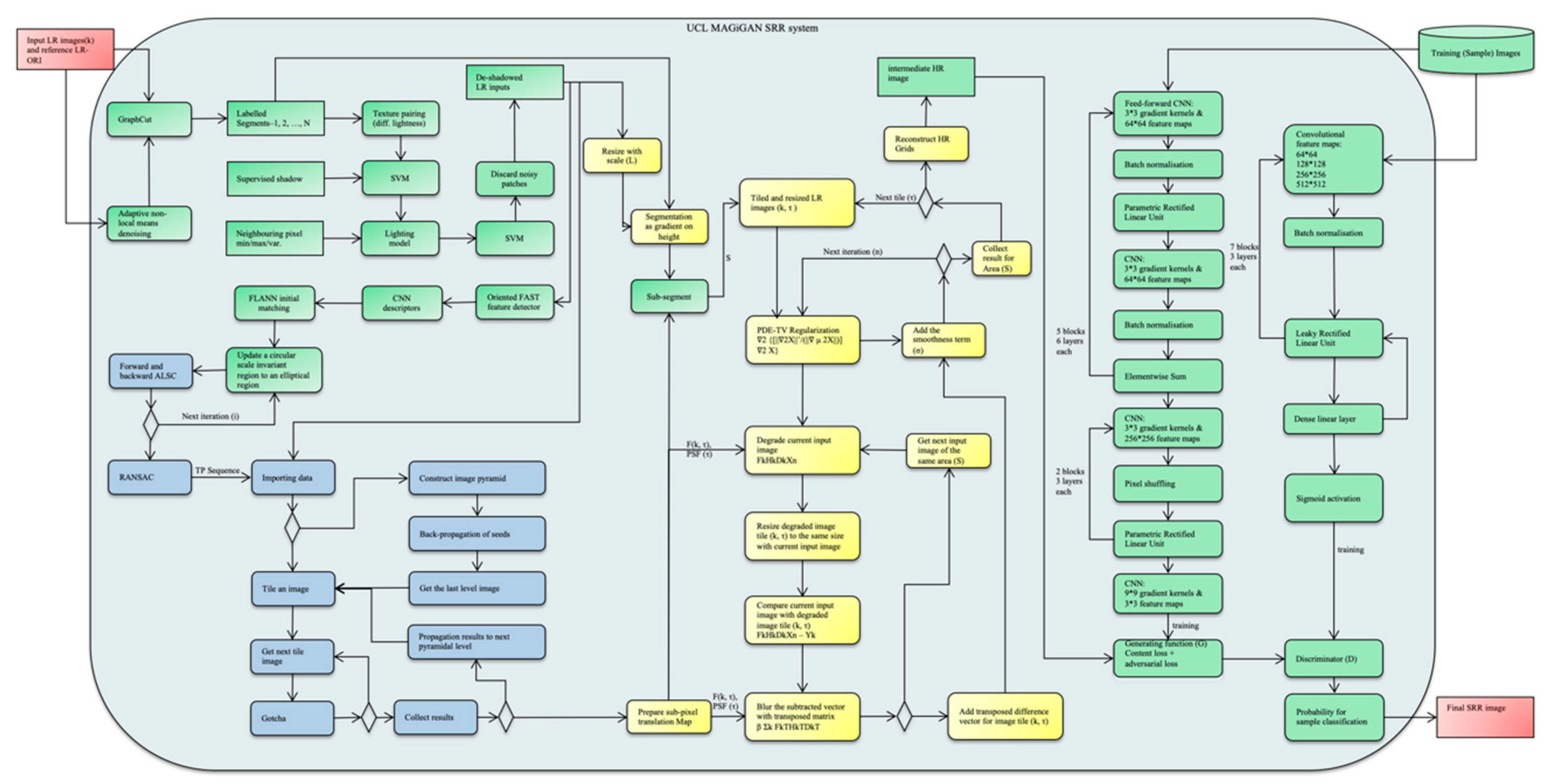
2.2. Methods

The MAGiGAN SRR system applied in this paper is based on our previous work of the GPT SRR system [6]. The GPT SRR system was previously demonstrated with experiments on 8 overlapping 25 cm NASA Mars Reconnaissance Orbiter (MRO) High-Resolution Imaging Science Experiment (HiRISE) images covering the Mars Exploration Rover (MER) Spirit rover traverse to resolve up to 5× higher spatial resolution [10]. The resulting resolution enhancement brought new surface information on individual rocks (diameter < 50 cm), rover tracks, and new evidence for the Beagle-2 lander using multi-angle HiRISE images [35,36]. However, when applying the original GPT SRR system to EO data including Urthecast Corp Deimos-2 images and SSTL Carbonite-2 video sequences, we were only able to achieve a resolution enhancement of about 2× due to changes in the Earth’s surface (e.g., vegetation phenology), shadow, and atmospheric obstacles. Also, GPT-SRR introduces information from multi-angles, but cannot retrieve high-texture detail as it is based on pixel wise differences. The new MAGiGAN SRR system is developed to address these problems by producing denser initial feature correspondences on de-shadowed input images and applying a deep learning image network to further refine the SRR result [1].

A detailed flow diagram of the MAGiGAN SRR system is shown in Figure 2. A simplified flow diagram can be found in [1]. The overall process of the MAGiGAN SRR system can be divided into 5 main stages, including:

(1)

Image segmentation and de-shadowing;

(2)

Initial feature matching and subpixel refinement;

(3)

Subpixel feature densification;

(4)

Estimation of the image degradation model;

(5)

GAN network training and SRR refinement (prediction).

Stage (1) pre-processes the LR inputs to intermediate de-shadowed segmented patches. This step aims to minimize the gaps in the motion maps caused by matching LR images with different shading effects for stage (2) and stage (3) processing. Stage (1) also prepares image segments for stage (4) restoration. Stage (2) produces accurate and evenly distributed initial feature correspondences between the LR images and the reference image. Stage (3) then densifies the feature correspondences from stage (2) and produce initial HR interpolated grid. Stage (4) iteratively refines the initial HR grid through estimation of image degradation models. Finally, the intermediate HR image from stage (4) is further refined via a trained GAN network at stage (5). Processing for each of the 5 stages is described in detail as follows.

Aside from these, image pre-denoising may be required for some datasets. This was initially discovered with the HiRISE GPT-SRR processing which showed that additional noisy LR scenes would reduce the overall quality of the SRR result. Within the CEOI SuperRes-EO project, we added an additional pre-denoising workflow to deal with datasets containing strong noise. Because noisy LR images produce less accurate sub-pixel feature correspondences and sparser (or invalid) motion vectors, it will result in inaccurate estimation of the degradation matrix at stage (4). Theoretically, the noisier the LR images which are used as inputs, the more “clear” LR images are needed for estimation of the HR “true scene”. When all input LR images are noisy, the noise data are generally magnified in the intermediate SRR image produced at the end of stage (4).

In MAGiGAN, we implemented an optional adaptive non-local means (ANLM) denoising step originally for SSTL Carbonite-2 processing, but can be used for any datasets that have continuous repeat observations. The ANLM method is based on the non-local means (NLM) denoising which takes a mean of all pixels in a sequence of images, weighted by how similar these pixels are to the target pixel. The NLM denoised value at a given pixel is obtained by a weighted average of the pixels in its temporal neighborhood. The temporal neighboring pixels are found by minimizing the mean squared difference (MSD) of a sliding window within a constrained step size (in x and y directions). ANLM uses the K-means clustered segments to replace the fixed sized sliding window in NLM in order to reduce the averaging effects and preserves image details.

In the UCL MAGiGAN SRR system, we take roughly aligned overlapping multi-angle LR images and a reference ortho-rectified image (ORI; if available) or (near-)nadir view image as inputs. A scaling factor of 2× is set for the intermediate HR image output at stage (3) and (4), a further scaling of 2× is set for the final SRR output at stage (5).

Firstly, at stage (1) image segmentation and de-shadowing, we aim to minimize the gaps on the motion maps caused by matching LR images with different shading effects and use image segmentation to restore different features separately. Differences in shading effects may be treated as image content differences (like clouds) when matching multiple LR images. At stage (3), gaps (unmatched regions) are forcibly interpolated using neighboring pixels on the HR grid. The de-shadowing process can significantly minimize interpolation of the initial HR grid, by helping to find seed feature correspondences (and later on densified) between LR images and the reference image, when there are differences in shadow orientation. For MISR SRR processing, the difference in shadow orientation is minor due to the short time delay between each adjacent LR images. However, producing de-shadowed intermediate images is important for other single camera instruments, especially for urban or forested areas.

In this work, an area-based image segmentation and de-shadowing process is applied. This stage (1) process is summarized as follows:

Segmentation of the LR images based on their image content using the GC algorithm [37];

(1.1)

Pair the segmented image patches for the same region from multiple LR images using normalized cross-correlation;

(1.2)

If paired segments are found with the same illumination, they should be labelled with the same shadow notation (either shadowed or non-shadowed);

(1.3)

If paired segments are found with different illumination, and one segment is much darker (at a given threshold) than the other one, the darker segment is labelled as a shadow;

(1.4)

Use a pre-trained SVM [38] classifier to correct the shadow labels produced from previous step in order to increase the confidence of the shadow labelling. Note that the SVM classifier is pre-trained using a small amount of manually selected shadowed and non-shadowed segments from the GC results;

(1.5)

Group the connected shadowed patches or non-shadowed patches to one shadow segment or one non-shadow segment;

(1.6)

Correct the illumination of the shadow segments using illumination statistics from the neighboring non-shadowed pixels. Note that not all shadow segments are correctable, the intensity (texture) information may already lost during imaging. Such shadow segments will have a very low signal to noise ratio (SNR) after de-shadowing. This means that there will be no (or only very few) added feature correspondences for that region after the de-shadowing process;

(1.7)

In case of irrecoverable shadowed segments, the de-shadowed segments are reversed back to their original intensities.

The de-shadowed intermediate images are only used as metadata to provide seed feature points for the shadowed regions and are not used in the follow-on processing stages. The output SRR will keep the shading information from the reference image which are not devoid of shadows. The segmented patches are passed through to the next processing stages for sub-segmentation based on the threshold of the maximum differences of the magnitude of the distance of the motion vectors. This is for further optimisation of the tiling process of the PDE-TV regularization step in order to restore different types of image content separately.

Secondly, at stage (2) initial feature matching and subpixel refinement, we aim to produce initial feature correspondences between LR images and the reference image for stage (3) processing, and then derive the initial HR grid (a scaled version of the reference image interpolated by LR images). An accurate, dense, and evenly distributed first estimation of the seed points is essential to the success of interpolating the initial HR grid. Ideally, the subpixel feature correspondences derived at this stage should be refined to an accuracy of 0.01 pixels and distributed evenly amongst different types of image content (e.g., building blocks, trees, roads, flat regions, shaded regions, and saturated regions). The UCL MAGiGAN SRR system uses a MSA-FAST-CNN [2,3,4] based feature matching approach to produce much denser initial feature correspondences (as well as at a higher processing speed) as described in [1] in comparison to the original GPT SRR system [6] which uses the scale invariant feature transform (SIFT) [39].

The MSA-FAST-CNN feature matching and subpixel refinement process of stage (2) can be summarized as follows:

(2.1)

Derive initial feature points by considering a circle of 16 pixels around a local maximal point, if 12 out of 16 pixels are all brighter or all darker than a given threshold from the center point, then record it as an initial feature point;

(2.2)

Refine the initial feature points using a pre-trained decision tree classifier (ID3 algorithm) to produce optimal choices of feature points;

(2.3)

Compare adjacent feature points according to their sum of absolute differences (SAD) between the feature points and 16 surrounding pixel values and discard the adjacent feature points with a lower SAD;

(2.4)

At each scale, extract circular patches of 15 by 15 pixels around each FAST feature points;

(2.5)

Use a pre-trained CNN model consisting of 3 convolutional layers, proposed in [40], to extract descriptors from all patches. The extracted descriptors include output vectors from all 3 convolutional layers and a fully connected layer;

(2.6)

Initial descriptor matching using a fast library for approximate nearest neighbor (FLANN);

(2.7)

Iteratively update the matched seed point locations and orientations from the previous step using forward and backward ALSC within a transformable elliptical window [2].

The MSA-FAST-CNN method produces much denser feature correspondences compared to the MSA-SIFT and MSA-SURF methods in our SRR experiments described in [1]. The feature correspondences are more evenly distributed between different types of image content including recovered shadow regions after stage (1) processing. The MSA method has an important impact on reconstructing the initial HR grid by correcting the FAST features detected independently in each image. This eliminates slight mismatches from significant image distortion caused by different viewing angles. A set of dense and accurate initial seed correspondences are essential to produce a more accurate motion map in the follow-on stage (3) and stage (4) processing.

Thirdly, at stage (3) subpixel feature densification, the optimized feature correspondences are then used as seed points in a pyramidal version of ALSC and region growing (Gotcha) process until most pixels in the LR images find their optimal subpixel correspondence with respect to the reference frame. These sub-pixel correspondences are collected to form a series of 2-channel motion maps with encoded subpixel x and y translation vectors. Pixels in any LR image that do not match with any subpixel location in the reference HR grid, are removed from the calculation in further steps. If a subpixel location in the HR grid does not have any corresponding motion vector from all motion maps, this HR pixel will be propagated by its neighboring HR pixels.

The Gotcha process of stage (3) can be summarized as follows:

(3.1)

Tile the LR images (ensuring that each tile has sufficient number of seed points) and construct image pyramids from coarse to fine resolution;

(3.2)

Run ALSC on the seed points and record their similarity value;

(3.3)

Sort seed tie-points by similarity value;

(3.4)

A new matching is derived from any adjacent neighbors of the initial tie-point with the highest similarity value;

(3.5)

If the new match is verified by ALSC then it is considered as a seed tie-point for the next region-growing iteration;

(3.6)

This region growing process repeats from (3.3) to (3.5) until there are no more acceptable matches at the current level of resolution;

(3.7)

Propagate the intermediate correspondences to the next finer resolution level and repeat from (3.2) to (3.6) until there are no more acceptable matches at the current level of resolution;

(3.8)

Collect the densified subpixel correspondences from all tiles.

The Gotcha method progressively refines the existing subpixel correspondences and densify until we find a matching for all valid pixels (LR pixels that cannot be matched due to image differences are discarded). At this processing stage, an initial HR grid is produced by scaling up the reference image and interpolated using transformed LR pixels. The dense subpixel correspondences for each LR images are stored as 2-channel matrices (initial motion maps). The motion maps provide the initial degradation information in the similarity measurement term of the MAP estimation at the next processing stage.

Fourthly, at stage (4) estimation of the image degradation model, we aim to iteratively refine the initial HR grid through estimation of a sequence of degradation matrices by minimizing the similarity cost (calculated from the MSD of each LR image and degraded HR image) and weighted regularization cost. This stage follows a MAP approach using PDE-TV regularization.

The PDE-TV regularization process of stage (4) is solved using a steepest descent method. This process is summarized as below:

(4.1)

LR images and the initial HR grid are segmented into tiles according to the segmented patches from stage (1) processing and sub-segmentation based on a given threshold of the maximum differences of the magnitude of the distance of the motion vectors;

(4.2)

For the same area, each tile (t) of an initial HR image is projected with motion vector (degradation matrix F), convolved with the first estimation of the Point Spread Function (PSF) (degradation matrix H) which is assumed to be a small Gaussian kernel with various standard deviations according to the size of the segment, down-sampled (degradation matrix D) with the defined scaling factor;

(4.3)

Compare the degraded image with each LR image (k) tile (t) sequentially;

(4.4)

Add the transposed difference vector to the HR grid tile (t);

(4.5)

Add the smoothness term and decompose the TV regularization term with a 4th order PDE;

(4.6)

Repeat from (4.2) by convolving the degradation matrices with updated HR image for the next steepest descent iteration until it converges, i.e., the differences in (4.3) is minimized;

(4.7)

Collect the HR result for this tile (t) and then go back to (4.2) for the next tile (t + 1) until all segments converge;

(4.8)

Post-processing including noise filtering and de-blurring.

A mathematical representation of this process can be found in [6]. The intermediate HR output image from stage (1) to stage (4) processing contains restored information from multi-angle distorted features contained in each LR input image. The intermediate HR image generally produces less resolution enhancement for regions that changed in each LR input than the regions that are comparably static. This means the effective resolution enhancement for the intermediate HR image (as well as the final SRR image) is not the same for different regions depending on the number of matched pixels from each LR input. Also, the intermediate HR image does not contain high frequency texture details for flat regions given that there is no multi-angle information. Artefacts might be found in areas which have difficulty in matching, for example, multiple views of a growing cloud when views are completely different from different viewing angles. These issues were observed in processing of the Deimos-2 images for the Dubai site for urban landscape features. The intermediate HR output image from the stage (4) processing will be used as input for the GAN refinement (prediction) at stage (5) processing.

Finally, at stage (5), GAN network training and SRR refinement, we further refine the intermediate HR image from stage (4) output using a pre-trained GAN network. GAN uses the perceptual loss calculated from feature maps of the deep learning network to replace the MSE-based content loss and is, therefore, highly complementary to the multi-angle feature matching and model-based approach in terms of restoring different features. In the UCL MAGiGAN system, the GAN single image SRR refinement step uses the SRR output from MSA-FAST-CNN-GPT. GAN applies a deep network (Generator G) to generate high frequency textures that are highly similar to real images, in combination with an adversarial network (Discriminator D) to distinguish super-resolved images from real images. In this work, we adapt the GAN architecture described in [9].

In this work, 135 full strip MISR An Red channel L1B2 images are used to form 225,282 HR training samples with size 256 × 256 (discarded bad scenes). 135 full strip MISR Af and Aa Red channel L1B2 images are Gaussian blurred and down-sampled to form 225,282 LR training samples with size 64 × 64 (discarded bad scenes).

The GAN training and prediction process of stage (5) is summarised as below:

(5.1)

Train a pair of the LR and HR images in the generator network;

(5.2)

Minimise the perceptual loss (containing the content loss and adversarial loss) in backpropagation of the generator network;

(5.3)

Calculate/update parameterised weights and biases of the generator network;

(5.4)

Generate a fake HR image using the generator network;

(5.5)

Train the discriminator network with the fake HR image and a real HR image;

(5.6)

Calculate discriminator loss in backpropagation of the discriminator network;

(5.7)

Update parameterised weights and biases of the discriminator network;

(5.8)

Record discriminator prediction and loss;

(5.9)

Update the adversarial loss in the generator network;

(5.10)

Repeat from (5.1) to (5.9) for all training pairs until the fake HR image is classified as a real HR image.

(5.11)

Generate the SRR image using the intermediate HR output from stage (4) with the fully trained GAN network.

The generator network uses residual blocks consisting of 2 convolutional layers with small 3 by 3 kernels and 64 feature maps followed by batch-normalisation layers for each residual block. The discriminator network contains 8 convolutional layers with 3 by 3 filter kernels and 64 to 512 feature maps. At this stage, we also applied the modifications suggested by [34] in order to balance the training strength between generator and discriminator. This includes removing the sigmoid activation from the discriminator network, not using the algorithm in the loss calculation of both generator and discriminator, constraining the weights to a constant range, and using stochastic gradient descent (SGD) to replace the momentum-based optimiser.

In this work, the LR images are pre-cropped to smaller sample sizes of 1024 × 1024 (maximum size we can handle is 2048 × 2048) pixels for the stage (1) to (4) processing. The resulting intermediate HR images (size 2048 × 2048) are then further divided into smaller sample sizes (128 × 128 pixels) to be used for GAN refinement, resulting in the final SRR images (size 256 × 256) with an overall up-scaling factor of 4×. The cropping (tiling) is mainly due to memory limitations of computation.

3. Results

In this paper, we demonstrate MISR SRR results from four test sites at the Railroad Valley, the U.S. Sky Zone Trampoline Park urban and countryside region, a sea ice field and a cloud field. For evaluation purpose, we applied two image quality metrics using the Landsat image as reference and two independent quality scoring systems (one with, and one without, a perceptual training model). 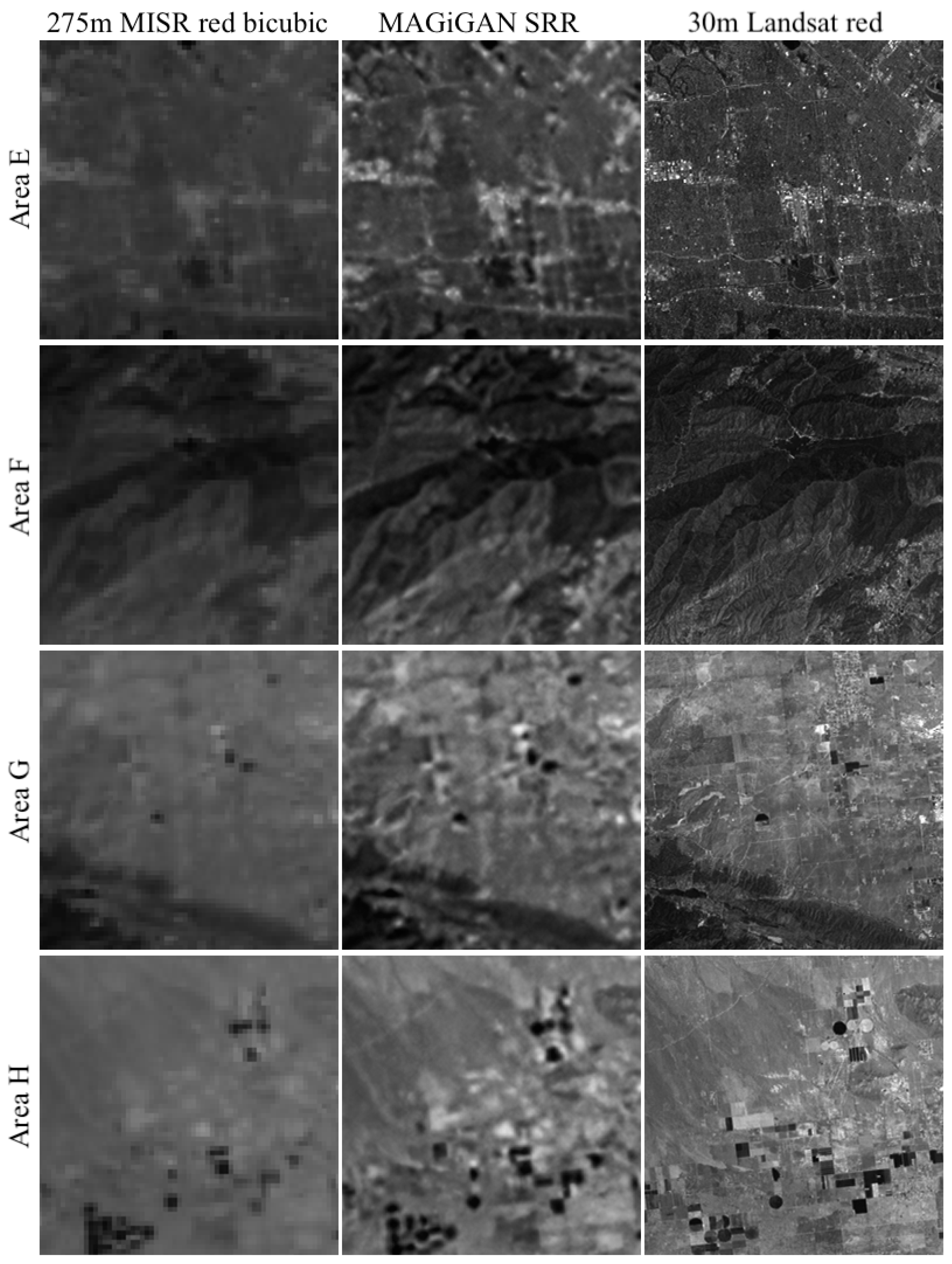These image quality metrics are as follows:

(1)

Peak signal-to-noise ratio (PSNR). PSNR is derived from the mean square error (MSE), and indicates the ratio of the maximum pixel intensity to the power of the distortion. However, PSNR and MSE metrics are based on pixel-wise difference, they may not be able to capture perceptual details (e.g., high-frequency textures). Mathematical equations for PSNR calculation can be found in [35].

(2)

Mean Structural Similarity Index Metric (mean SSIM) [41]. SSIM combines local image structure, luminance, and contrast into a single local quality score. In this metric, structures are patterns of pixel intensities, especially among neighboring pixels, after normalizing for luminance and contrast. Because the human visual system is good at perceiving structure, the SSIM quality metric agrees more closely with the subjective quality score. Structural similarity is computed locally, a mean SSIM value of the overall image performance is calculated. Mathematical equations for mean SSIM calculation can be found in [42].

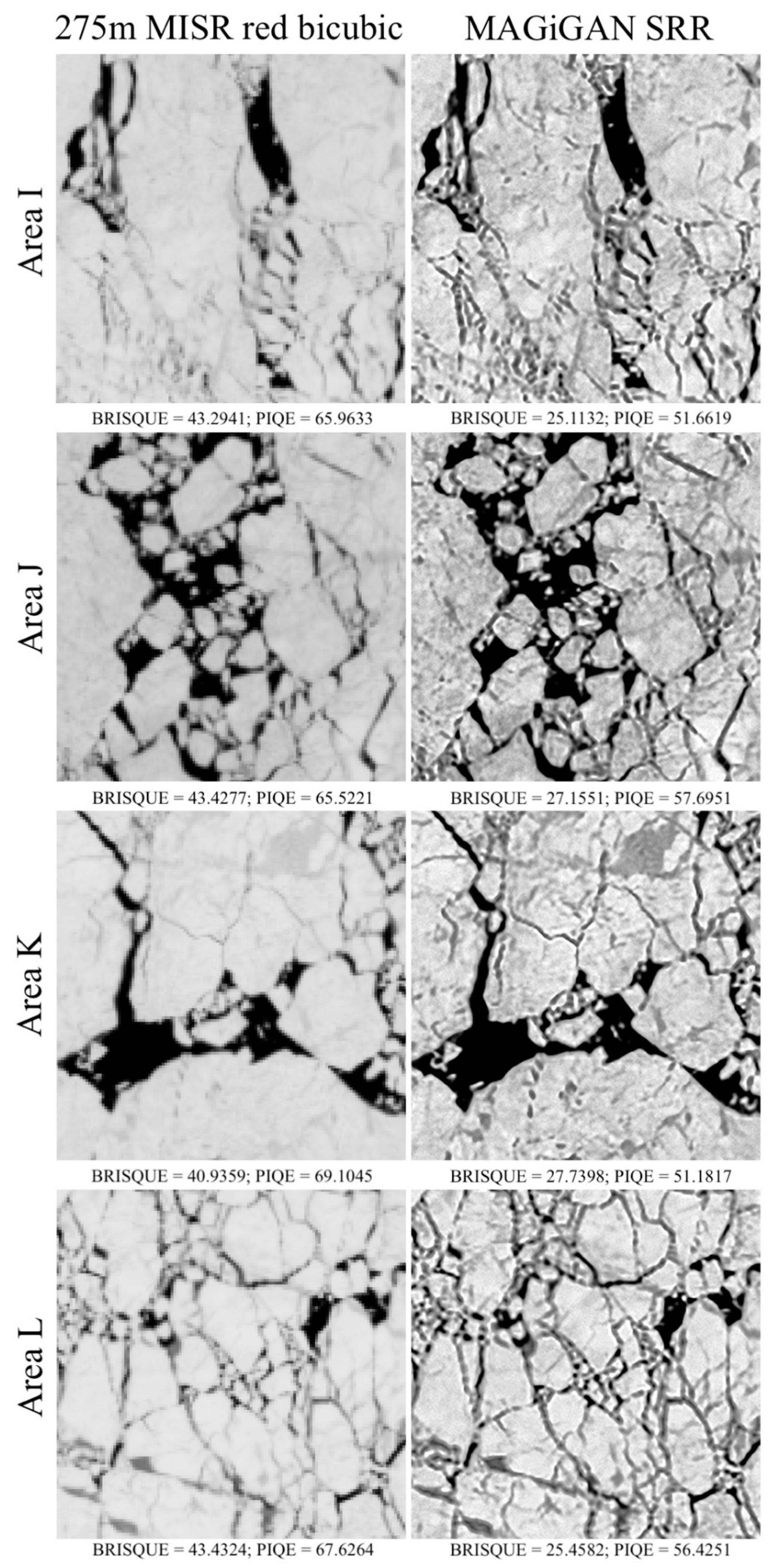
(3)

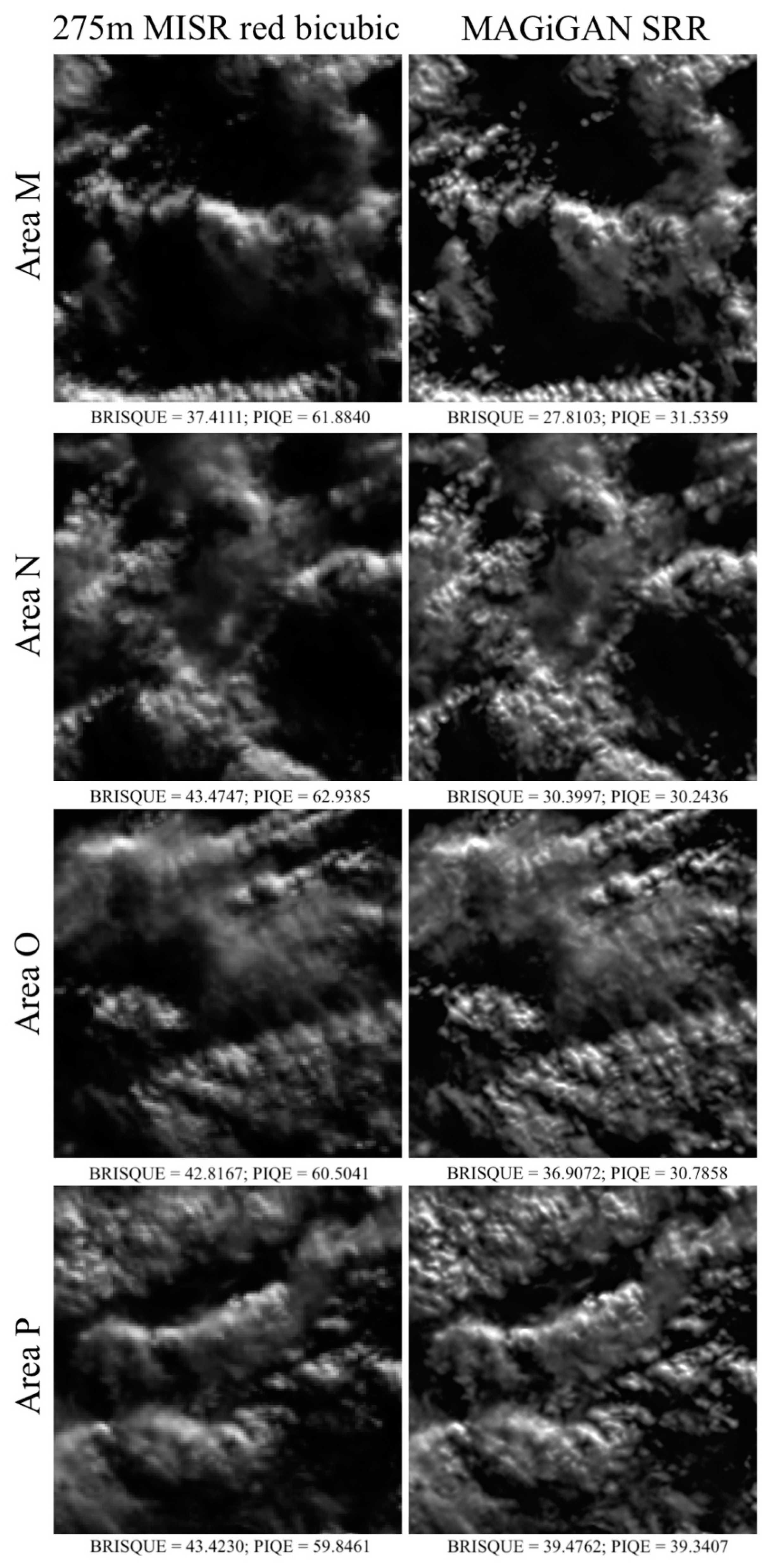
Blind/Referenceless Image Spatial Quality Evaluator (BRISQUE) [43]. The BRISQUE model provides subjective quality scores based on a training database of images with known distortions. The score range is between 0 and 100. Lower values reflect better perceptual quality.

(4)

Perception-based Image Quality Evaluator (PIQE) [44]. The PIQE algorithm is opinion-unaware and unsupervised, which means it does not require a trained model. PIQE can measure the quality of images with arbitrary distortion. PIQE estimates block-wise distortion and measures the local variance of perceptibly distorted blocks to compute the quality score. The score range is between 0 and 100. Lower values reflect better perceptual quality.

The first test site Railroad Valley is an EO vicarious calibration test site with large homogenous regions located at (38.5°, −115.69°) in the state of Nevada, U.S. In this work, we take cropped 275 m MISR red band L1B1 images with 8 off-nadir viewing angles (P040_O044742_DF/CF/BF/AF/AA/BA/CA/DA_F03_0024) and 1 red band L1B2 reference image (P040_O044742_AN_F03_0024), taken on 16 May 2008, as inputs to produce output SRR image at 4× scaled grid (68.75 m) with an effective resolution of about 3×. The 30 m Landsat 7 red band image (LE07_L1TP_040033_20080516_20160923_01_T1_B3), taken on the 16 May 2008, is used for comparison with the SRR result. A comparison of the UCL MAGiGAN SRR results at Railroad Valley in comparison with the original 275 m MISR red band image and 30 m Landsat red band image for 4 different areas are shown in Figure 3.

Table 1. Statistics of the image quality metrics for the bicubic interpolated MISR red band input reference image, SRR results, and the Landsat 7 red band validation reference image for the 4 areas in the first testing site.

Area	Image	Peak Signal-to-Noise Ratio (PSNR)	Mean Structural Similarity Index Metric (SSIM)	Blind/Referenceless Image Spatial Quality Evaluator (BRISQUE) %	Perception-Based Image Quality Evaluator (PIQE) %
A	MISR red band bicubic	26.7346	0.7416	52.0543	66.1779
	SRR	29.1094	0.8619	39.6647	19.7091
	Landsat red band	-	1.0	20.2014	8.1027
B	MISR red band bicubic	23.2949	0.5639	53.4357	63.1433
	SRR	22.1310	0.7496	45.5916	28.4979
	Landsat red band	-	1.0	19.1740	14.9896
C	MISR red band bicubic	24.3419	0.7443	47.6324	54.6479
	SRR	32.2880	0.8497	39.2999	30.8875
	Landsat red band	-	1.0	5.9161	10.8337
D	MISR red band bicubic	26.2917	0.7161	49.2402	62.3354
	SRR	27.0486	0.8538	42.0864	25.5005
	Landsat red band	-	1.0	16.9750	9.1723

shows the statistics of the image quality metrics for the bicubic interpolated MISR red band input reference image, SRR results, and the Landsat 7 red band validation reference image for the 4 areas (A, B, C, D) of the first test site at Railroad Valley. The Landsat 7 red band validation image is used as the reference image for calculating the PSNR and mean SSIM value of the MISR and SRR image. The SRR images achieved higher PSNR for Areas A, C, and D compared to the bicubic interpolated MISR images. The PSNR of the SRR image is slightly lower for Area B compared to the bicubic interpolated MISR image. However, the PSNR measurement is inconclusive as it is based on pixel wise differences with respect to a much higher resolution “truth” and it is not able to capture the perceptual details. The higher mean SSIM values of the SRR images for all four areas reflect that the SRR images contain more structural features which are observable in the Landsat image. The mean SSIM values agree more closely with the human perceptual resolution compared to PSNR. The BRISQUE and PIQE measurements provide image quality scores between 0 to 100 (lower values reflect better perceptual quality). The difference is that BRISQUE uses a pre-trained image quality scoring model (using real LR and HR images), whereas PIQE is based on known image distortions. The SRR images have better scores for both BRISQUE and PIQE measurement for all four areas compared to the bicubic interpolated MISR images. Although, as expected, the much higher resolution Landsat images have the best scores overall.

At the second test site, we used the urban and countryside region around the Sky Zone Trampoline Park, located at (34.21°, −118.49°) northwest of Los Angeles, CA in the U.S. In this work, we took cropped 275 m MISR red band L1B1 images with 8 off-nadir viewing angles (P040_O044742_DF/CF/BF/AF/AA/BA/CA/DA_F03_0024) and 1 red band L1B2 reference image (P040_O044742_AN_F03_0024), taken on the 16 May 2008, as inputs to produce output SRR image at 4× scaled grid (68.75 m) with effective resolution of about 3.5×. The 30 m Landsat 7 red band image (LE07_L1TP_041036_20080608_20160918_01_T1_B3), taken on the 8 June 2008, is used for comparison with the SRR result. A comparison of the UCL MAGiGAN SRR results at Sky Zone Trampoline Park urban and countryside region in comparison with the original 275 m MISR red band image and 30 m Landsat red band image for 4 different areas are shown in Figure 4.

Table 2. Statistics of the image quality metrics for the bicubic interpolated MISR red band input reference image, SRR results, and the Landsat 7 red band validation reference image for the 4 areas in the second testing site.

Area	Image	PSNR	Mean SSIM	BRISQUE %	PIQE %
E	MISR red band bicubic	22.8083	0.4086	43.4232	62.1026
	SRR	23.9358	0.6045	31.3546	57.5544
	Landsat red band	-	1.0	20.4667	20.7558
F	MISR red band bicubic	27.3632	0.5964	43.2030	72.2120
	SRR	27.2719	0.7147	35.8270	69.0694
	Landsat red band	-	1.0	28.4648	10.5390
G	MISR red band bicubic	20.7561	0.4630	43.4571	64.9261
	SRR	25.0931	0.6471	34.7673	57.8650
	Landsat red band	-	1.0	25.0066	11.5139
H	MISR red band bicubic	18.9588	0.4824	43.4566	59.0510
	SRR	22.3327	0.6772	32.8828	60.4824
	Landsat red band	-	1.0	25.9460	11.5531

shows the statistics of the image quality metrics for the bicubic interpolated MISR red band input reference image, SRR results, and the Landsat 7 red band validation reference image for the 4 areas (E, F, G, H) of the second test site at the Sky Zone Trampoline Park. The corresponding Landsat 7 red band validation image is used for calculating the PSNR and mean SSIM value of the MISR and SRR image. The SRR images achieved better overall PSNR, mean SSIM, BRISQUE and PIQE scores compared to the bicubic interpolated MISR images, except for two outliers (PSNR at Area F and PIQE at Area H).

At the third test site, we picked a sea ice field located at (76.9°, −142.6°). In this work, we took cropped 275 m MISR red band L1B1 images with 8 off-nadir viewing angles (P080_O039735_DF/CF/BF/AF/AA/BA/CA/DA_F03_0024) and 1 red band L1B2 reference image (P080_O039735_AN_ F03_0024), taken on the 7 June 2007, as inputs to produce output SRR image at 4× scaled grid (68.75 m) with effective resolution of about 2.75×. There is no Landsat image available of that area for evaluation. A comparison of the UCL MAGiGAN SRR results for the sea ice field in comparison with the original 275 m MISR red band image for 4 different areas are shown in Figure 5, the corresponding BRISQUE and PIQE scores are given below each image. The SRR image contains more structural details and sharper edges compared to the bicubic interpolated MISR image. The SRR image achieved good overall scores for both BRISQUE and PIQE for all 4 areas (I, J, K, L) of the third testing site at the sea ice field. In particular, leads and meltwater ponds can be observed in the MISR SRR which are difficult to detect in the original MISR scene.

At the last test site, we picked a cloud field located using the same MISR orbit (P080_O039735_F03_0024) captured on the 7 June 2007. The output SRR image is 4× scaled grid (68.75 m) with an effective resolution of about 2.75×. There is no Landsat image available around the same time for evaluation. A comparison of the UCL MAGiGAN SRR results for the cloud field in comparison with the original 275 m MISR red band image for 4 different areas are shown in Figure 6, the corresponding BRISQUE and PIQE scores are given below each image. The SRR image contains more structural and texture details compared to the bicubic interpolated MISR image. The SRR image achieved much better scores for both BRISQUE and PIQE compared to the bicubic interpolated MISR image for all 4 areas (M, N, O, P) of the fourth testing site at the clouds field.

The example results from the 4 test sites (Railroad Valley, Sky Zone Trampoline Park, sea ice field, and cloud field) have shown restoration (resolution enhancement) of different types of features (e.g., urban buildings, roads, rural places, calibration targets, sea ice, and clouds) from the MISR images. Although the SRR image quality or resolution enhancement factor may not be the same across the whole image subject to many different factors (e.g., feature matching completeness and accuracy, image obstacles and noise, and sufficient training data) which have been discussed in the methods section (Section 2.2), the SRR image achieved better overall scores using 4 different image quality/resolution measurement methods compared to the bicubic interpolated MISR image and is tending towards the very high-resolution Landsat image.

4. Discussion

SRR of EO imagery is more challenging than Mars imagery [6] due to frequent changes in the Earth’s surface, atmosphere clarity, shadowing, and more complex artificial structures. In this paper, we introduce the UCL MAGiGAN SRR system, developed within the CEOI SuperRes-EO project, designed to address various issues found with EO SRR. The overall quality of the MAGiGAN SRR results for EO data are generally affected by 4 factors: (1) the quality of the input LR images; (2) the number of LR images; (3) the time difference between each LR image; (4); a sufficient volume of training data(sets); (5) image obstacles in terms of smoke, haze, and clouds. The MISR data is considered ideal for the MAGiGAN SRR system, because the issues from (1)–(4) are generally minor. By manually or automatically selecting obstacle-free (or -less) input LR images, issues from (5) can be ignored as well.

We demonstrate restoration of different types of higher resolution image content including urban and rural targets, sea ice and clouds using MISR L1B1 red band images at 4 different sites. A rich set of SRR training data (containing 225,282 LR samples and 225,282 HR samples) was employed for the GAN processor using MISR L1B2 red band images. The SRR results showed different image quality and effective resolutions, depending on how well the different types of image content have been trained. In the future, we aim to collect a much larger training dataset combining different image sources at different resolutions to produce better SRR results. Ideally, larger training datasets can be split into multiple categories according to the different types of image content using an automatic image content classification algorithm. For example, in our previous experiments with Urthecast Corporation Deimos-2 images [1], we used two sets of training data (manually selected) for SRR of urban and rural scenes. Given the rich global repeat coverage of MISR images, and future possibilities of combining a multiple imaging source, a better classified training database is expected to benefit the SRR work. It is also feasible that multiple repeat MISR images could be employed to enhance the resolution further.

The input LR images used for the 4 test sites are extracted from two MISR orbits (44,742 and 39,735). Four different image quality/resolution measurement methods based on the overall image performance are used to compare the SRR results with the original MISR input image and higher resolution Landsat image, where available. During the evaluation stage, significant resolution improvement over rural places has been observed. We are also able to retrieve detailed textures for near featureless areas. It was determined that an increase in resolution of up to a factor of 3.5 could be achieved with a minimal stack of 8 off-nadir images based on the MISR experiments introduced in this paper and previous experiments with other EO imagery in [1].

The multi-angle feature matching and model-based approaches applied in the MAGiGAN SRR system and the GAN single image SRR process are highly complementary to each other in terms of restoring different types of features. If only GAN is applied [9] then there is a risk that artificial features will be “detected” falsely. This is demonstrated in Figure 7, where in the lower right corner of the central pivot irrigation (CPI) features one of the dark spots is misidentified as one of these features, which is clearly not the case in the Landsat 30 m image. However, when GAN is applied to the intermediate HR output from the multi-angle feature restoration and image degradation modelling approach shown in the MAGiGAN figure below then this does not occur. Therefore, the GAN single image SRR process was integrated as a further refinement step within the MAGiGAN SRR system. An example is shown of a comparison of the SRR results (4× upscale) produced from our previous GPT SRR algorithm [6], the GAN single image SRR algorithm (4× upscale) [9], and the proposed MAGiGAN SRR algorithm (4× upscale) in Figure 7, for an area close to the satellite calibration target at the Railroad Valley, NV site. Reference images including the original MISR and Landsat images and a downsampled Landsat image at 68.75 m are also included. In this visual comparison, we can see that the GPT SRR is able to restore the structural information of the CPI targets but is not able to restore high frequency texture details, whereas the GAN SRR result shows more texture details than the GPT SRR result. The GAN SRR result (4× upscale) shows sharper edges of the CPI targets compared to the GPT SRR result (4× upscale), but the textures and edges are not consistent when compared to the Landsat truth image. For example, the textures at the top left corner has a mixture of signal and noise. The MAGiGAN SRR result (4× upscale) is visually the most similar to the 68.75 m downsampled Landsat truth image. The MAGiGAN SRR result (4× upscale) has shown that using GAN as a refinement process (2× upscale) for the intermediate HR image (2× upscale), produced from our multi-angle feature restoration and image degradation modelling approach, generated the best overall structural and texture restoration quality and reduced unreliable synthesis (artefacts) arising from pure machine learning-based methods.

According to the BRIQUE and PIQE evaluation criteria, we achieved the best overall SRR results for the Railroad Valley site, satisfactory results for the cloud field, and similar quality for the Sky Zone Trampoline Park site and sea ice field. For the Railroad Valley and Sky Zone Trampoline Park site, we are able to compare the restored structural features with higher resolution Landsat images. The SRR images from the Railroad Valley site also restored the most structural features according to the mean SSIM measurements. In addition, the regional resolution of an SRR image depends on the local feature matching accuracy and changes (including obstacles) of the region within each LR acquisition. The evaluation of an enhancement factor of the SRR result may not be represented by an overall evaluation metric or measurement of a single object due to the nature of the feature-based approach.

5. Conclusions

In this paper, we introduced the implementation details of the recently developed UCL MAGiGAN SRR system which is based on multi-angle feature restoration, image degradation modelling, and deep learning refinement processes. The UCL MAGiGAN SRR system takes advantage of both the photogrammetric restoration approach and deep learning techniques to restore both multi-angle distorted features and higher-frequency textures. We demonstrated using the multi-angle 275 m red band MISR L1B1 and LIB2 images that SRR images at 4× scaled grid (68.75 m) with an effective resolution of between 2.75× to 3.5×.

Examples are provided over 4 test sites, including a satellite vicarious calibration site at Railroad Valley, nearby urban and countryside scenes at the Sky Zone Trampoline Park site, a sea ice field, and a cloud field. Multiple evaluation methods are introduced and applied to the SRR results and the validation images from Landsat 7.

Most components of the UCL MAGiGAN system have been ported onto a space-qualified GPU board (NVIDIA Jetson TX-2) for speeding up the processing within the recently completed CEOI SuperRes-EO project. This also allows potential future tests of the SRR onboard a “smart satellite”.

Future work will include (1) GPU porting of the Gotcha process (or develop an equivalent algorithm that is better suited for parallel processing); (2) forming much richer LR/HR training datasets for different types of targets using multiple imaging sources; and (3) a test of how far we can use SRR onboard in future EO missions. As far as MISR is concerned, an evaluation will be conducted of the potential of MISR SRR to be used to detect sea ice floe leads and melt-ponds with a view to linking the surface bi-directional anisotropy of the sea ice reflectance variation with these features and their link to sea ice surface roughness.

References

- Tao, Y.; Muller, J.-P. Repeat multiview panchromatic super-resolution restoration using the UCL MAGiGAN system. In Proceedings of the Image and Signal Processing for Remote Sensing XXIV 2018, Berlin, Germany, 10–13 September 2018; Volume 10789. Issue 3. [Google Scholar]
- Tao, Y.; Muller, J.-P.; Poole, W.D. Automated localisation of Mars rovers using co-registered HiRISE-CTX-HRSC orthorectified images and DTMs. Icarus 2016, 280, 139–157. [Google Scholar] [CrossRef]
- Rosten, E.; Drummond, T. Machine Learning for High-Speed Corner Detection. Comput. Vis. 2006, 3951, 430–443. [Google Scholar] [Green Version]
- Fischer, P.; Dosovitskiy, A.; Brox, T. Descriptor matching with convolutional neural networks: A comparison to SIFT. ArXiv, 2014; arXiv:1405.5769. [Google Scholar]
- Shin, D.; Muller, J.-P. Progressively weighted affine adaptive correlation matching for quasi-dense 3D reconstruction. Pattern Recognit. 2012, 45, 3795–3809. [Google Scholar] [CrossRef]
- Tao, Y.; Muller, J.-P. A novel method for surface exploration: Super-resolution restoration of Mars repeat-pass orbital imagery. Planet. Space Sci. 2016, 121, 103–114. [Google Scholar] [CrossRef]
- Bouzari, H. An improved regularization method for artefact rejection in image super-resolution. SIViP 2012, 6, 125–140. [Google Scholar] [CrossRef]
- Guo, R.; Dai, Q.; Hoiem, D. Single-image shadow detection and removal using paired regions. In Proceedings of the IEEE Conference on CVPR 2011, Colorado Springs, CO, USA, 20–25 June 2011; pp. 2033–2040. [Google Scholar]
- Ledig, C.; Theis, L.; Huszár, F.; Caballero, J.; Cunningham, A.; Acosta, A.; Aitken, A.P.; Tejani, A.; Totz, J.; Wang, Z.; et al. Photo-Realistic Single Image Super-Resolution Using a Generative Adversarial Network. CVPR 2017, 2, 4. [Google Scholar]
- Tao, Y.; Muller, J.-P. Quantitative assessment of a novel super-resolution restoration technique using HiRISE with Navcam images: How much resolution enhancement is possible from repeat-pass observations. ISPRS Int. Arch. Photogramm. Remote Sens. Spat. Inf. Sci. 2016, 41, 503–509. [Google Scholar] [CrossRef]
- Irwin, R.; (Urthecast Corp, Vancouver, Canada); Rampersad, C.; (Urthecast Corp, Vancouver, Canada). Personal communication, 2018.
- Jovanovic, V.; Smyth, M.; Zong, J.; Ando, R. MISR Photogrammetric Data Reduction for Geophysical Retrievals. IEEE Trans. Geosci. Remote Sens. 1998, 36, 1290–1301. [Google Scholar] [CrossRef]
- Mahlangu, P.; Mathieu, R.; Wessels, K.; Naidoo, L.; Verstraete, M.; Asner, G.; Main, R. Indirect Estimation of Structural Parameters in South African Forests Using MISR-HR and LiDAR Remote Sensing Data. Remote Sens. 2018, 10, 1537. [Google Scholar] [CrossRef]
- Duchesne, R.R.; Chopping, M.J.; Tape, K.D.; Wang, Z.; Barker Schaaf, C.L. Changes in tall shrub abundance on the North Slope of Alaska 2000–2010. Remote Sens. Environ. 2018, 219, 221–232. [Google Scholar] [CrossRef]
- Scanlon, T.; Greenwell, C.; Czapla-Myers, J.; Anderson, N.; Goodman, T.; Thome, K.; Woolliams, E.; Porrovecchio, G.; Linduška, P.; Smid, M.; et al. Ground comparisons at RadCalNet sites to determine the equivalence of sites within the network. In Proceedings of the SPIE 8660 Digital Photography 2017, Melbourne, Australia, 10–13 December 2017. [Google Scholar]
- Tsai, R.Y.; Huang, T.S. Multipleframe Image Restoration and Registration. In Advances in Computer Vision and Image Processing, Greenwich; JAI Press Inc.: New York, NY, USA, 1984; pp. 317–339. [Google Scholar]
- Keren, D.; Peleg, S.; Brada, R. Image sequence enhancement using subpixel displacements. In Proceedings of the IEEE Conference on Computer Vision and Pattern Recognition 1988, Ann Arbor, MI, USA, 5–9 June 1988; pp. 742–746. [Google Scholar]
- Alam, M.S.; Bognar, J.G.; Hardie, R.C.; Yasuda, B.J. Infrared image registration and high-resolution reconstruction using multiple translationally shifted aliased video frames. IEEE Trans. Instrum. Meas. 2000, 49, 915–923. [Google Scholar] [CrossRef]
- Takeda, H.; Farsiu, S.; Milanfar, P. Kernel regression for image processing and reconstruction. IEEE Trans. Image Process. 2007, 16, 349–366. [Google Scholar] [CrossRef]
- Hardie, R.C.; Barnard, K.J.; Armstrong, E.E. Joint MAP registration and high resolution image estimation using a sequence of undersampled images. IEEE Trans. Image Process. 1997, 6, 1621–1633. [Google Scholar] [CrossRef] [PubMed]
- Yuan, Q.; Zhang, L.; Shen, H. Multiframe super-resolution employing a spatially weighted total variation model. IEEE Trans. Circuits Syst. Video Technol. 2012, 22, 379–392. [Google Scholar] [CrossRef]
- Farsiu, S.; Robinson, D.; Elad, M.; Milanfar, P. Fast and robust multi-frame super-resolution. IEEE Trans. Image Process. 2004, 13, 1327–1344. [Google Scholar] [CrossRef] [PubMed]
- Purkait, P.; Chanda, B. Morphologic gain-controlled regularization for edge-preserving super-resolution image reconstruction. Signal Image Video Process. 2013, 7, 925–938. [Google Scholar] [CrossRef]
- Kumar, S.; Nguyen, T.Q. Total subset variation prior. In Proceedings of the IEEE International Conference on Image Processing 2010, Hong Kong, China, 26–29 September 2010; pp. 77–80. [Google Scholar]
- Elad, M.; Datsenko, D. Example-based regularization deployed to super-resolution reconstruction of a single image. Comput. J. 2007, 52, 15–30. [Google Scholar] [CrossRef]
- Dong, C.; Loy, C.C.; He, K.; Tang, X. Learning a deep convolutional network for image super-resolution. In Proceedings of the ECCV 2014, Zurich, Switzerland, 6–12 September 2014; pp. 184–199. [Google Scholar]
- Osendorfer, C.; Soyer, H.; Smagt, P. Image super-resolution with fast approximate convolutional sparse coding. In NIPS 2014; Springer: Cham, Switzerland, 2014; pp. 250–257. [Google Scholar]
- Yang, J.; Wang, Z.; Lin, Z.; Cohen, S.; Huang, T. Coupled dictionary training for image super-resolution. IEEE TIP 2012, 21, 3467–3478. [Google Scholar]
- Kim, J.; Lee, J.K.; Lee, K.M. Deeply-recursive convolutional network for image super-resolution. In Proceedings of the IEEE Conference on Computer Vision and Pattern Recognition (CVPR) 2016, Las Vegas, NV, USA, 26 June–1 July 2016; pp. 1637–1645. [Google Scholar]
- Radford, A.; Metz, L.; Chintala, S. Unsupervised representation learning with deep convolutional generative adversarial networks. ArXiv, 2015; arXiv:1511.06434. [Google Scholar]
- Lei, S.; Shi, Z.; Zou, Z. Super-resolution for remote sensing images via local–global combined network. IEEE Geosci. Remote Sens. Lett. 2017, 14, 1243–1247. [Google Scholar] [CrossRef]
- Lanaras, C.; Bioucas-Dias, J.; Galliani, S.; Baltsavias, E.; Schindler, K. Super-resolution of Sentinel-2 images: Learning a globally applicable deep neural network. ArXiv, 2018; arXiv:1803.04271. [Google Scholar]
- Pouliot, D.; Latifovic, R.; Pasher, J.; Duffe, J. Landsat Super-Resolution Enhancement Using Convolution Neural Networks and Sentinel-2 for Training. Remote Sens. 2018, 10, 394. [Google Scholar] [CrossRef]
- Arjovsky, M.; Chintala, S.; Bottou, L. Wasserstein GAN. ArXiv, 2017; arXiv:1701.07875. [Google Scholar]
- Matlab Page for PSNR Equation. Available online: https://uk.mathworks.com/help/images/ref/psnr.html (accessed on 6 December 2018).
- Bridges, J.C.; Clemmet, J.; Pullan, D.; Croon, M.; Sims, M.R.; Muller, J.-P.; Tao, Y.; Xiong, S.-T.; Putri, A.D.; Parker, T.; et al. Identification of the Beagle 2 Lander on Mars. R. Soc. Open Sci. 2017, 4, 170785. [Google Scholar] [CrossRef] [PubMed]
- Rother, C.; Kolmogorov, V.; Blake, A. GrabCut: Interactive foreground extraction using iterated graph cuts. In Proceedings of the ACM SIGGRAPH 2004, Los Angeles, CA, USA, 8–12 August 2004; pp. 309–314. [Google Scholar]
- Chang, C.-C.; Lin, C.-J. LIBSVM: A library for support vector machines. ACM Trans. Intell. Syst. Technol. 2011, 2, 1–27. [Google Scholar] [CrossRef]
- Lowe, D.G. Distinctive image features from scale-invariant keypoints. Int. J. Comput. Vis. 2004, 60, 91–110. [Google Scholar] [CrossRef]
- Dosovitskiy, A.; Fischer, P.; Springenberg, J.T.; Riedmiller, M.; Brox, T. Discriminative unsupervised feature learning with exemplar convolutional neural networks. IEEE Trans. Pattern Anal. Mach. Intell. 2016, 38, 1734–1747. [Google Scholar] [CrossRef] [PubMed]
- Zhou, W.; Bovik, A.C.; Sheikh, H.R.; Simoncelli, E.P. Image Qualifty Assessment: From Error Visibility to Structural Similarity. IEEE Trans. Image Process. 2004, 13, 600–612. [Google Scholar]
- Matlab Page for SSIM Equation. Available online: https://uk.mathworks.com/help/images/ref/ssim.html (accessed on 6 December 2018).
- Mittal, A.; Moorthy, A.K.; Bovik, A.C. No-Reference Image Quality Assessment in the Spatial Domain. IEEE Trans. Image Process. 2012, 21, 4695–4708. [Google Scholar] [CrossRef] [PubMed] [Green Version]
- Venkatanath, N.; Praneeth, D.; Chandrasekhar, B.M.; Channappayya, S.S.; Medasani, S.S. Blind Image Quality Evaluation Using Perception Based Features. In Proceedings of the 21st National Conference on Communications (NCC) 2015, Mumbai, India, 27 February–1 March 2015. [Google Scholar]