Abstract
Due to the availability of observations and the effectiveness of bias correction, it is still a challenge to assimilate data from the polar orbit satellites into a limited-area and frequently updated model. This study assessed the initial application of satellite radiance data from multiple platforms in the Rapid-refresh Multi-scale Analysis and Prediction System (RMAPS). Satellite radiance data from the advanced microwave sounding unit-A (AMSU-A) and microwave humidity sounding (MHS) were used. Two 12-day retrospective runs were conducted to evaluate the impact of assimilating satellite radiance data on 0–24 h forecasts using RMAPS. The forecasts, initialized from analyses with and without satellite radiance data, were verified against observations. The results showed that satellite radiance data from AMSU-A and MHS had a positive impact on the initial conditions and the forecasts of RMAPS, even over the relatively data-rich area of North China. Compared to the control run that only assimilated conventional observations, an improvement of about 36.8% can be obtained for the temperature bias between 300 hPa and 850 hPa and 0.65% for the average RMSE. Satellite radiance observations from 1200 UTC contribute relatively significantly (77.8%) to the bias improvement of the initial temperature field. For the wind at 10 m, the bias and root-mean-square error (RMSE) both had a reduction for the 0–12 h forecast range. An improvement can be also found for the skill score of the 3-h accumulated rainfall below 10.0 mm in the first 12 h of the forecast range. There was a slight improvement in the skill score of the 6-h accumulated rainfall above 50 mm over North China, with a 20.7% improvement for the first 12 h of the forecast. The inclusion of satellite radiance observations was found to be beneficial for the initial temperature, which consequently improved the forecast skill of the 0–12 h range in the RMAPS.
1. Introduction
Currently, weather situational-awareness requirements for increased accuracy in short-range weather forecasts are increasing. The accuracies of forecasts produced by regional numerical weather prediction (NWP) models rely critically on two conditions [1]: the intrinsic laws and the initial state of the atmosphere. The basic conservation laws and atmospheric motion equations form the theoretical support for the intrinsic atmospheric laws, which successfully produce weather forecasts for current global and regional NWP models [2]. However, improving the accuracy of the initial state of the atmosphere is still a challenge. To produce an accurate initial state, which is known as an analysis, observational data are generally optimally combined with a short-range forecast from the previous analysis via a process known as data assimilation [3,4].
Weather observations can be broadly divided into conventional observations and those from satellites. Most conventional instruments make direct measurements of atmospheric variables from surface stations, radiosonde, and aircraft over populated land regions. These observations are always local and have a patchy distribution [3], being most dense in East Asia, North America, and Europe. Satellites can provide measurements for much of the globe within a short period of time, either for nearly a hemisphere (from a geostationary orbit) or for the entire globe twice a day (from a polar orbit). Even over populated areas, satellite observations are able to fill the gaps between the radiosonde locations and their launch times. Based on recent studies [2,5,6], contributions from satellite data, especially from infrared and microwave sounders, are increasingly becoming the most important observations in operational centers. Since satellite instruments do not directly measure the atmospheric parameters used in the NWP model, the assimilation of satellite data can be complex [3,7,8]. One approach is to assimilate the retrieved data, such as temperature, humidity and wind, from radiances measured by the satellite instruments. However, this conversion process is mathematically ill-posed and usually requires extra prior information and restrictive assumptions [9]. The second approach is to directly assimilate the satellite radiances via a forward radiative transfer model [10,11,12], which calculates the radiance from the vertical profiles of the model. With the development of fast radiative transfer models, radiances from various satellite instruments have been directly assimilated in most operational NWP centers based on variational data assimilation schemes [9,13,14,15,16]. These satellite radiance observations provide 90–95% of the actively assimilated data for global models and significantly improve the NWP skill [17,18]. In current NWP systems, satellite radiance observations are becoming the most important data source used to improve the short- and medium-range forecast quality [3,19].
Compared to global models, regional satellite radiance assimilation is not yet a fully developed field [10]. For the polar orbit satellites, limited satellite data coverage and effectiveness of regional bias correction are key challenges for assimilating radiance data into the limited-area and frequently updated models [20]. Due to the limited data swaths and the limited extent of the domain, the non-uniform data coverage results in a highly variable number of available observations per cycle, which can reduce the effectiveness of bias correction in the regional model. Another factor is complications resulting from local and diabatic effects, complex nonlinear balance relationships, and the presence of lateral boundaries, which require using a dynamical approach for data analysis and assimilation [21,22]. Due to these complications and operational forecasting requests for regional scales, satellite radiance data assimilation for initialization in regional models has received the most attention [10]. Many studies have been performed to evaluate the impact of satellite radiance on the skill of weather forecasts in regional models. McNally et al. [23] investigated the role of satellite radiance data in the forecasting of European Centre for Medium-Range Weather Forecasts (ECMWF) and found that polar-orbit satellite data play an important role in decreasing the time and location errors of hurricane-track forecasts. Groverasmussen [24] indicated that assimilating microwave radiance measurements over land and sea-ice was expected to result in a further positive impact, based on the system implemented at the Danish Meteorological Institute, most noticeably at high latitudes. Lin et al. [25] provided a recent upgraded assimilation of the polar orbiter and geostationary satellite radiance data in the Rapid Refresh (RAP) and High-Resolution Rapid Refresh (HRRR) operational models and indicated that a positive impact had been seen in retrospective runs with the new radiance data.
This study aims to assess the initial application of satellite radiance data from multiple polar orbit platforms in a regional NWP model, Rapid-refresh Multi-scale Analysis and Prediction System (RMAPS), which is running operationally at the Beijing Meteorological Bureau. Currently, considerable amounts of conventional and radar observations are included in the data assimilation system of RMAPS. This study further investigates the added value from satellite radiance data in the scope of the RMAPS, mainly over China region. Satellite radiance data of the microwave sounding AMSU-A and MHS from NOAA-18/19 and Metop-B were selected and integrated into RMAPS. Two 12-day retrospective runs over the period of 1–12 August 2017, with and without satellite radiance data assimilation, were conducted and compared. Components of the upper-air, near surface, and precipitation from the forecasts were investigated and evaluated against ground and sounding observations. The rest of this paper is organized as follows: Section 2 describes the regional model of RMAPS, radiance data assimilation, satellite observations, verification data, and strategies that were used in this study; Section 3 provides the details of the two experimental retrospective runs; Section 4 presents the study results and discussion; and the conclusions are given in Section 5.
2. Materials and Methods
2.1. Model Description
RMAPS is a rapid-refresh multi-scale analysis and prediction system, which has run operationally at the Beijing Meteorological Bureau since 2015. It was developed by the Institute of Urban Meteorology in the China Meteorological Administration in collaboration with the National Center for Atmospheric Research (NCAR). RMAPS uses the advanced research WRF (ARW) model and WRF data assimilation (WRFDA) of version 3.8.1 [14,26,27]. In particular, the land-use data in RMAPS has 33 modified categories based on USGS (the United States Geological Survey) data, which has higher accuracy and finer classification over urban areas. The background error covariance used for data assimilation is generated based on forecasts over a period of one month for different seasons using the NMC (National Meteorological Center) method [28].
The fundamental configurations for RMAPS are given in Table 1. There are two nested domains in RMAPS, as shown in Figure 1. Domain 1 covers the entire China region, with a grid spacing of 9 km and 649 × 500 grid points. Domain 2 is centered on North China with a grid spacing of 3 km and 550 × 424 grid points. There are 50 vertical computational layers with a pressure top of 50 hPa. Atmospheric and surface fields from the European Centre for Medium-Range Weather Forecasts (the EC forecasts) are introduced as the initial conditions of RMAPS. The physics schemes include Thompson double moment microphysics, ACM2 PBL, Kain-Fritsch deep convection, the RRTMG shortwave and longwave scheme, and the Unified Noah land-surface model. A three-dimension variational (3DVar) technique is used for the data assimilation. Conventional observations in 3-h cycling assimilation provide the analysis fields for RMAPS, including SYNOP (conventional grounded-based, site distributions shown as the red points in Figure 1), METAR (airport ground-based), SHIP (ship based), BUOY (oceanographic buoys), AMDAR (aircraft-based), RAOB (sounding), PILOT (a pilot balloon system), and GPSZTD (ground-based GPS zenith total delay) observations. In addition to conventional data, radial velocity and reflectivity from radar observations are also assimilated in the Domain 2.

Table 1.
Model and configurations of RMAPS.
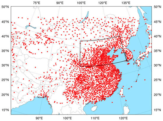
Figure 1.
The domains of RMAPS. The outside box indicates Domain 1 and the inner black box indicates Domain 2. The red points represent the distribution of the ground sites.
2.2. Radiance Data Assimilation
The basic idea of data assimilation is to combine complementary information from observations with an NWP product (the first guess or background), and thus produce an optimal estimate of the atmospheric state (the analysis). A variety of methods, such as three/four dimension variational (3DVar/4DVar) and ensemble Kalman filter (EnKF) methods, have been developed to achieve the best possible analysis for a forecast model [29,30,31]. In this study, the 3DVar method is used for the satellite radiance data assimilation. In 3DVar data assimilation, the problem can be summarized as the iterative minimization of a prescribed cost-function (1) to find the analysis sate that minimizes [32].
Here, the background and observations are the two given sources of a priori data. , , and F are the background, observation (instrumental), and representivity error covariance matrices, respectively. Meanwhile, an observation operator is introduced to transform the gridded analysis to observation space as for comparison with observations. This solution represents a posteriori maximum likelihood estimate of the true sate of the atmosphere.
For satellite radiance data assimilation, the observation operator is a radiative transfer model that calculates radiances from the model data. In this study, the community radiative transfer model (CRTM) [12] is used for the radiance data assimilation in RMAPS. For channels with a significant thermally emitted contribution, the top of the atmosphere upwelling clear-sky radiance at a given frequency and viewing angle can be computed based on the following expression [11]:
where is the surface to space transmittance, is the surface emissivity, is the Planck function, is the surface radiative temperature, and is the layer mean temperature.
In addition, since radiances measured by satellites are not obviously linked to atmospheric or surface temperatures, they are usually converted to brightness temperatures (Tb) for data assimilation via Plank function inversion [33].
2.3. Satellite Radiance Observations
The satellite radiance observations used in this study were from AMSU-A and MHS instruments mounted on the polar-orbiting satellites NOAA-18/19 and METOP-A/B. The centeral frequency of each channel and the corresponding peaks of response/weight functions (WFs) are listed in Table 2 [34]. AMSU-A has an instantaneous field-of-view of 3.3° at half-power points, and the spatial resolution at nadir is nominally 48 km. It has 15 measurement channels in total of which 4 (channels 1–3, and 15) measure energy primarily from the surface and the boundary layer, while the remaining 11 channels are “temperature sounding” channels that primarily provide atmospheric temperature information [35]. MHS has an instantaneous field of view of 1.1° at the half-power points, with a nominal spatial resolution of 16 km at nadir. It has five channels of which two (channels 1 and 2) measure in the spectral “window” regions. Channels 3–5 are “humidity sounding” channels that can be used to derive atmospheric humidity profiles.
Table 2.
Channel frequencies and peaks of weight functions (WFs) for AMSU-A and MHS.
A polar-orbiting satellite may make measurements from the same location just once or twice a day. However, similar measurements can be obtained from a given location many times a day by the same sensors carried on multiple polar platforms [23]. Figure 2 shows the coverages of AMSU-A channel 6 from the satellites NOAA-18, NOAA-19, and METOP-B used in RMAPS on 11 August 2017. It can be seen that there are observations covering the area at each analysis time in the 3-h cycling assimilation.
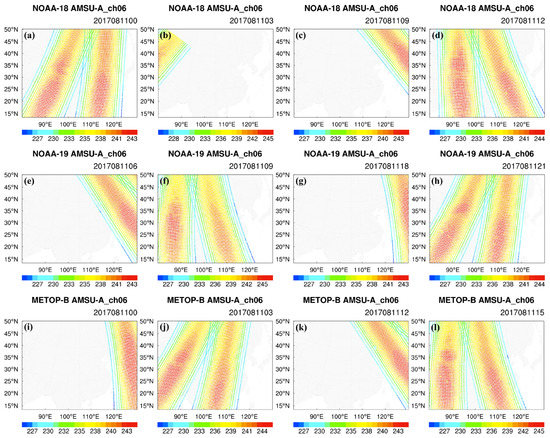
Figure 2.
The coverages of AMSU-A channel 6 from satellites NOAA-18 (a–d), NOAA-19 (e–h), and METOP-B (i,j,k and l) used in RMAPS on 11 August 2017, at different times. Different colors denote the brightness temperatures (K) from the satellite radiance observations.
2.4. Verification Data
First, ground observations from automatic weather stations (AWS) were used for verification and the distribution of these ground sites is shown in Figure 1. Reliable surface temperature, humidity, and precipitation amounts (using rain gauges) with high temporal frequency can be obtained from AWS [36]. To match the forecast grid point values to the observation points in the horizontal plane, the forecast value was assigned the value at the nearest grid point for comparison.
Second, conventional radiosonde observations were used for comparison and evaluation. Figure 3 shows the spatial distribution of the radiosonde observations in Domain 1. In the vertical direction, if any discrepancy existed between the vertical levels of forecasts and observations, then the forecasts were interpolated to the level of the observation. The vertical interpolation was done in natural log of pressure coordinates, except for specific humidity, which was interpolated using the natural log of specific humidity in natural log of pressure coordinates. If forecasts and observations were at the same vertical level, then they were directly paired.
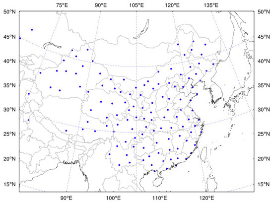
Figure 3.
The spatial distribution of the radiosonde observations used for verification (123 points).
2.5. Verification Strategy
To assess the application of satellite radiance data assimilation in RMAPS, several standard verification statistics were used. Four statistical indices were used to verify the rainfall forecasts, including the critical success index (CSI or Threat Score), the bias score (BIAS), the probability of detection (POD), and the false alarm ratio (FAR). In addition, the bias and root-mean-square error (RMSE) were used to evaluate the vertical temperature and humidity profiles and the surface components of the forecasts.
For quantitative precipitation forecasting, a four-cell contingency table (Table 3) can be used to describe the relationship between the forecasts and the observed events [37,38]. Consider a set of forecasts that only has two alternative statements: yes and no. In this case, denotes the number of hits; denotes the number of false alarms; c denotes the number of misses; and d denotes the number of correct rejects. Then, CSI, BIAS, POD, and FAR can be defined as functions of , , c, and d, as listed in Table 4. The CSI explains how well the forecast “yes” events correspond to the observed “yes” events. BIAS indicates whether the forecast system has a tendency to under-predict (BIAS < 1) or over-predict (BIAS > 1) events. POD is the percent of events that were correctly forecast, and FAR is the ratio of the number of false alarms to the total number of predicted events.
Table 3.
Four-cell contingency table.
Table 4.
Statistical performance measures used for evaluation and comparison.
3. Assimilation Experiments
3.1. Experimental Design
To investigate the impact of satellite radiance data assimilation in RMAPS, two retrospective runs, a control (CTRL) run without satellite radiances and an experimental run (DA_RAD) with satellite radiance observations, were conducted over a 12-day (1–12 August 2017) period. These CTRL and DA_RAD runs started at 0000 UTC on 1 August 2017, when the initial conditions from the EC forecasts were introduced into RMAPS after a 6-h spin up, as shown in Figure 4. DA_RAD used all data, including the satellite radiance data, and CTRL used all data excluding the satellite radiance data. A 3-h cycling configuration was adopted as used operationally, and a 24-h forecast was produced for each 3-h cycle, yielding a total of 96 forecasts for each retrospective run.
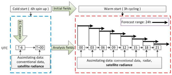
Figure 4.
A schematic of the retrospective run with satellite radiance observations in RMAPS.
The DA_RAD run included the assimilation of all of the observations used in the CTRL run plus the satellite radiance data. The radiance data were assimilated in RMAPS through the CRTM. All these observations were assimilated using a 3-h time window. In addition, radar observations were only assimilated in Domain 2 for the CTRL and DA_RAD runs.
3.2. Quality Control
In this study, a series of quality control (QC) procedures were also performed for the assimilation of the satellite radiance data, including limb adjustment, observation error statistics, channel selection, cloud detection, data thinning, and bias correction.
First, satellite radiance observations were checked for gross errors and departures from the background, and observations with brightness temperatures lower than 150 K or higher than 350 K were removed. Further, observations were discarded if the bias-corrected innovation (observation minus background) exceeded three times the standard deviation of the observation error. In addition, channels that have a peak energy contribution height above the vertical limit of the NWP model were not used in the data assimilation. Surface-sensitive window channels were also not assimilated, but used for cloud detection and verification. Scattering index and cloud liquid water were used to eliminate any observations that were contaminated. The differences of brightness temperatures between channel 1 and 15 of AMSU-A were used for the scattering index, and the cloud liquid water can be derived from the window channels. Second, redundancy in the data may cause correlated errors and computational expense; therefore, a data thinning of 120 km (map observations to the two-dimensional thinning grid points) was performed to reduce the data volume while retaining all of the useful information in the data assimilation system. Finally, radiance data with a systematic bias need to be properly corrected prior to assimilation. Modeling of the errors in the satellite radiances is usually expressed as a linear combination of a set of predictors [39,40], which is used to modify the forward operator:
where and denote the ith predictor and the corresponding bias correction coefficients, respectively. Bias correction parameters can be estimated within the variational assimilation, jointly with the atmospheric model state [9,41]. Five predictors were used, i.e., the scan position, which can be the index of the pixel in the field of view, the 1000–300 hPa and 200–50 hPa layer thicknesses, the surface skin temperature, and the total column water vapor.
4. Results and Discussion
In this section, the results of the retrospective assimilation experiments based on RMAPS are described. The details of all the figures and a discussion of the results are also given in this section.
4.1. Results
4.1.1. Analysis Statistics
Before examining the impacts of the bias-corrected satellite radiance data assimilation on forecasts in RMAPS, we first evaluated the analysis statistics by comparing the calculated brightness temperatures from the forecast background () and the analysis () to the corresponding values from radiance observations (). Figure 5 shows a time series of the 3-h OMB (observation minus background) and OMA (observation minus analysis) statistics for AMSU-A channel 6 and MHS channel 3 from NOAA-18. The statistics involve a somewhat varying number of data day by day because the data availability varies with the satellite passages. The mean biases after bias correction (OMB_wb) are obviously reduced compared to the values prior to correction (OMB_nb) for AMSU-A channel 6, but little or even increased for the MHS channel 3. The standard deviations (Stdv) of OMA are smaller than the corresponding values for OMB_wb for both instruments, notably for MHS channel 3. After the bias correction, the average errors of the analysis (OMA) were closer to zero, indicating that the bias correction is effective. Therefore, the analysis results can fit the satellite radiance observations well in RMAPS.
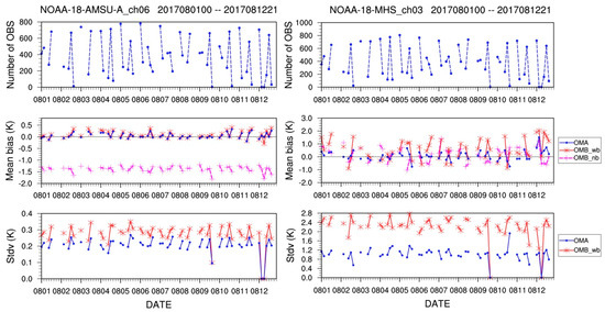
Figure 5.
The number of observations, mean bias, and standard deviation (Stdv) of AMSU-A channel 6 and MHS channel 3 of NOAA-18 for OMB without (OMB_nb) and with (OMB_wb) bias correction and OMA, valid from 0000 UTC on 1 August 2017, to 2100 UTC on 12 August 2017. OMB: observation minus background; OMA: observation minus analysis.
Figure 6 shows the statistics of the channels for AMSU-A and MHS from NOAA-18 at 0000 UTC on 11 August 2017. The channels that are sensitive to the surface were not used for the assimilation because they usually have large errors and uncertainty. QC removes the channels that contain significant amplitudes from the surface (channels 1–4, and 15 for AMSU-A and channels 1 and 2 for MHS) and that are over the vertical limit of RMAPS (channels 10–14 for AMSU-A), 50 hPa. Also, channels that have high bias and RMSE values when compared with derived results from the first guess fields should not be considered for assimilation. Therefore, we can see that the radiance observations assimilated in RMAPS are primarily from channels 5–8 of AMSU-A and channels 3–5 of MHS. After the bias correction (BC), the mean biases of each channel were reduced for AMSU-A but were increased for channels 4 and 5 of MHS. The Stdv of OMA is noticeably reduced for both AMSU-A and MHS. Figure 7 shows the scatter plots of the calculated brightness temperatures (Tb) versus observations. It can be seen that RMSE of the background with BC decreased from 1.281 K to 0.298 K (by 76.7%) compared to the results prior to BC. Compared to the results from the background, the RMSE and Stdv of the analysis are both reduced and the correlation coefficient between the results of the analysis and the observations slightly increased from 0.996 to 0.998.
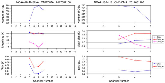
Figure 6.
The number of observations, mean bias, and standard deviation (Stdv) of all channels in the AMSU-A and MHS instruments from NOAA-18 for OMB without (OMB_nb) and with (OMB_wb) BC and OMA at 0000 UTC on 1 August 2017. OMB: observation minus background; OMA: observation minus analysis.
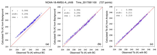
Figure 7.
Scatter plots of the brightness temperatures (Tb) calculated from the background (a) without and (b) with BC and (c) the analysis versus observations for AMSU-A channel 6 of NOAA-18.
4.1.2. Verification and Evaluation
For each retrospective run in this study, ninety-six 24 h forecasts were conducted based on RMAPS, including 96 analyses. We first calculated the average bias and RMSE of the atmospheric temperature and humidity (the water vapor mixing ratio, Qv) from the forecasts versus the observations. Figure 8 shows the average bias and RMSE of the vertical temperature profiles at hours 00, 06, 12, and 18 h of the forecasts. At the analysis time of 00 h, the satellite radiance data assimilation improved the temperature field between 300 hPa and 850 hPa. Compared to CTRL, the average bias is reduced from –0.19 to –0.12 K (approximately 36.8%), and only an improvement of about 0.65% is for the average RMSE with the value reduced from 0.926 to 0.920 K. At hours 06, 12, and 18 of the forecasts, the temperature bias between 300 hPa and 400 hPa experienced an overall reduction when including the satellite radiance data. A small improvement can be also found for 850 hPa at hour 06 and 12 of the forecast. For the average RMSE, a small improvement appears between 200 hPa and 400 hPa in the first 18 h of the forecasts, and an average reduction from 1.11 to 1.07 K is for 300 hPa. In Figure 9, the average bias and RMSE of the humidity are compared for CTRL and DA_RAD. It can be seen that the average bias of the humidity is increased below 400 hPa when using the satellite radiance data assimilation for the forecasts. For the average RMSE of the humidity profiles, there is almost no difference between the two retrospective run forecasts.
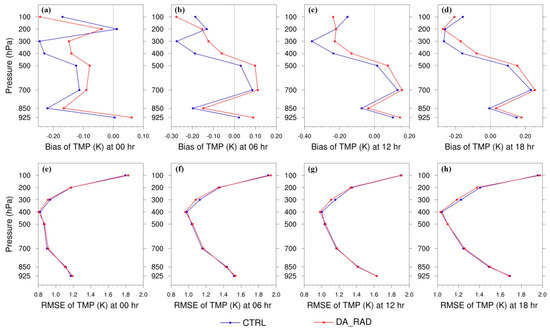
Figure 8.
The average bias (a–d) and RMSE (e–h) of the vertical temperature (TMP) profiles at hours 00, 06, 12, and 18 for retrospective run forecasts (over the period of 1–12 August 2017) without (CTRL) and with (DA_RAD) satellite radiances.
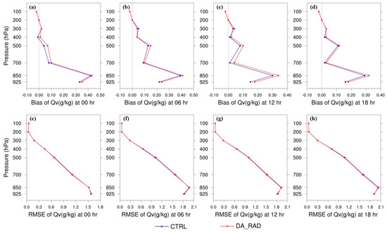
Figure 9.
The average bias (a–d) and RMSE (e–h) of the vertical humidity (Qv: water vapor mixing ratio) profiles at hours 00, 06, 18, and 24 of the forecasts for retrospective runs (over the period of 1–12 August 2017) without (CTRL) and with (DA_RAD) satellite radiances.
Figure 10 shows the time series of the 3-h average bias and RMSE for several forecast surface components, including the wind at 10 m and temperature (TMP) and humidity (Qv) at 2 m. Compared to CTRL, the satellite radiance data assimilation had a slight positive impact on the wind speed at 10 m for the forecast range of 0–12 h, the average bias was reduced from 1.14 to 1.12 m/s and the RMSE from 2.17 to 2.16 m/s. For the temperature at 2 m, there is almost no difference for the average bias and RMSE between the two retrospective runs, except for a small decrease in the RMSE at 00 h in DA_RAD. For the humidity at 2 m, the average bias increased after 6 h in DA_RAD and the average RMSE has a slight overall increase for the 24-h forecast range including the satellite radiances.
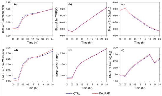
Figure 10.
Time series of the 3-h average bias and RMSE for (a,d) wind at 10 m and (b,e) temperature (TMP) and (c,f) humidity (Qv: water vapor mixing ratio) at 2 m for retrospective run forecasts over the period of 1–12 August 2017.
To further explore the impact of the satellite radiance observations in RMAPS, we investigated forecasts at different starting times. Because radiosonde observations were available every 12 h, we selected two groups of forecasts that started at 0000 UTC (2017080100–2017081200) and 1200 UTC (2017080112–2017081212) for further investigation. There are twelve 24-h forecasts included in CTRL and DA_RAD for each group. Figure 11 shows the average bias and RMSE of the vertical temperature profiles at the analysis time of 00 h for the forecasts in the two groups. Compared to CTRL, the average bias of the temperature between 300 hPa and 850 hPa in DA_RAD was improved in both groups; however, the improvement in the RMSE was tiny. For the forecasts started at 0000 UTC, the value in DA_RAD is reduced from 0.24 to 0.21 K (approximately 12.5%) for the bias and from 0.910 to 0.905 K (approximately 0.55%) for the RMSE compared to that of CTRL. For the forecasts started at 1200 UTC, an improvement in DA_RAD can be found below 200 hPa for the average bias of the temperature with the value reduced from 0.09 to 0.02 K (approximately 77.8%), and from 0.88 to 0.87 K (approximately 1.14%) for the average RMSE between 300 hPa and 850 hPa. Figure 12 shows the average bias and RMSE of the wind at 10 m for the two groups. Compared to CTRL, the average bias and RMSE in DA_RAD have an improvement of 1.2% and 0.5% in the first 12 h for the group of forecasts started at 0000 UTC, and 2.4% and 0.9% for the group of forecasts started at 1200 UTC. That is, satellite radiance observations from 1200 UTC contribute relatively significantly to the improvement in the initial temperature field and the wind at 10 m, even though the improvement is very small.
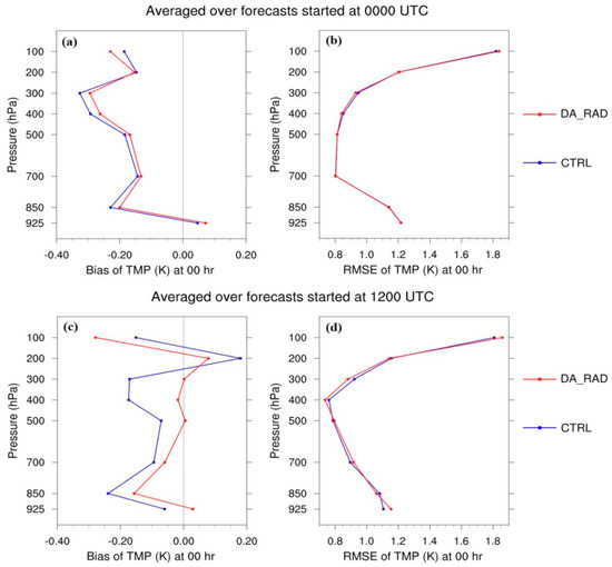
Figure 11.
The averaged bias and RMSE of the temperature (TMP) vertical profiles at the analysis time 00 h for forecasts started at (a,b) 0000 UTC and (c,d) 1200 UTC.
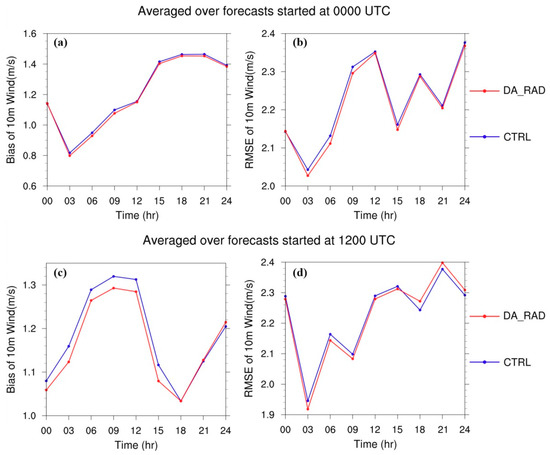
Figure 12.
The 3-h average bias and RMSE of the wind at 10 m for forecasts started at (a,b) 0000 UTC and (c,d) 1200 UTC.
In addition, observations from ground stations and rainfall scores were used to evaluate the impact of satellite radiances on the rainfall forecasting skill in RMAPS. The rainfall scores were averaged over ninety-six 24 h forecasts during the experimental period. Figure 13 shows the average CSI, BIAS, and FAR for the 3-h accumulated precipitation in Domain 1 with thresholds of 1.0 mm, 5.0 mm, and 10.0 mm. Compared to CTRL, the average CSI score in DA_RAD has an improvement in the first 12 h of the forecast range, with 2.0%, 3.0% and 2.9% for the thresholds of 1.0 mm, 5.0 mm and 10.0 mm, respectively. There is a corresponding decrease in the average BIAS score, especially for the first 6 h. The value is reduced from 2.96 to 2.70 for 1.0 mm, from 2.50 to 2.39 for 5.0 mm and from 1.89 to 1.79 for 10.0 mm in the first 6 h. However, the BIAS scores are still above 1.0 for both CTRL and DA_RAD, which is indicative of an over prediction for all thresholds. This indicates that the satellite radiance data assimilation provides a small improvement for over-prediction, leading to an improvement in the rainfall forecast skill below 10.0 mm for the first 12 h in RMAPS. Consistently, the FAR indices of DA_RAD also decreased in the first 12 h of the forecast range compared to the values of CTRL, but the improvements are all below 1%. This suggests that the false-prediction fraction was a little smaller for DA_RAD than for CTRL below 10.0 mm for the 3-h accumulated precipitation.
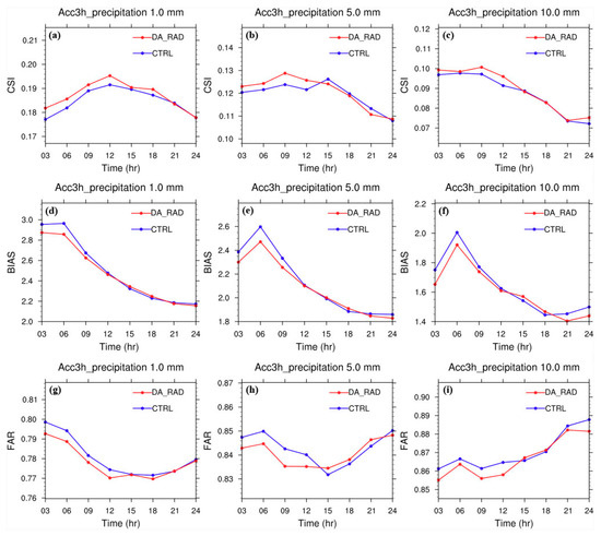
Figure 13.
Figure13. The average CSI (a–c), BIAS (d–f), and FAR (false alarm ration) (g–i) for the 3-h accumulated precipitation in Domain 1 with thresholds of 1.0 mm, 5.0 mm, and 10.0 mm.
Figure 14 further displays the average CSI and POD indices of the 6-h accumulated precipitation in Domain 2 for different thresholds for the first 12 h of the forecasts. It can be seen that the CSI and POD indices have a similar tendency. They both rapidly decrease with increasing threshold. Below the threshold of 25.0 mm, the rainfall skills of the forecasts with and without satellite radiances are roughly equivalent for CTRL and DA_RAD with similar CSI scores. For the threshold above 50 mm, the average CSI score in DA_RAD increased to 0.080 from 0.066 (approximately 20.7%) over the forecast range of 0–12 h, even though the value is still small (below 0.1). There is a corresponding increase for the POD, from 0.15 to 0.19 (approximately 22.8%). From the skill scores of the 6-h accumulated precipitation, we can see that the satellite radiance data assimilation in RMAPS has a slight positive impact on the heavy rainfall forecast over North China, which is covered by Domain 2.
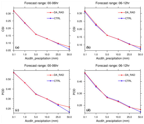
Figure 14.
The average CSI (a,b) and POD (c,d) for the 6-h accumulated precipitation in Domain 2 for different thresholds in the first 12 h of the forecasts.
4.2. Discussion
The results suggest that assimilating satellite radiance observations reduces the temperature bias in the troposphere at the analysis time in RMAPS. An improvement of about 36.8% can be obtained for the temperature bias between 300 hPa and 850 hPa. The wind at 10 m is also improved in the first 12 h of the forecast range. Consequently, there is a corresponding improvement in the skill scores for the 3-h accumulated rainfall below 10.0 mm in the first 12 h of the forecast range in RMAPS. Meanwhile, satellite radiance data assimilation improves the skill score of the 6-h accumulated rainfall above 50 mm over North China. However, uncertainties and several problems still need to be discussed.
First, the verification and assessment of forecast results were performed based on ground and sounding observations. The spatial distribution and number of observations directly influences the effect of the assessment. For example, only more than 100 sounding observations are available for comparison every 12 h (at 0000 UTC and 1200 UTC). In addition, these observations were interpolated onto the model grid points and vertical levels for comparison; therefore, representative errors exist.
Second, satellite radiance data assimilation improves the temperature of the middle and low levels at the analysis time but increases the humidity bias. The “humidity sounding” MHS can provide information about atmosphere humidity. Nevertheless, the results of the analysis statistics suggest that the biases after correction increased for the MHS channels. The channels of 3–5 used in data assimilation have the peak of response functions below 400 hPa, which correspond to the increased errors of humidity profiles in the middle and low levels. Therefore, further studies need to focus on the uncertainty of the impact from the MHS radiance data assimilation on forecasts in RMAPS.
Finally, improvements can be found for the initial temperature and the forecast skill from the application of satellite radiances in RMAPS; however, these positives are still limited to short forecasts of 24 h. Observations from AMSU-A and MHS can provide some information about temperature and humidity which are not enough for accurate short-term forecasting. For the initial conditions, an improvement of 36.8% can be found for the average bias of the temperature with satellite radiances, but only 0.65% for the average RMSE. For the forecasts, although there was an improvement for the skill scores below the rainfall of 10.0 mm in the first 12 h, the values in CTRL and DA_RAD were both still very low. This problem may be related to the verification techniques in which the spatial and the presence of features in the forecast fields were not considered [38]. For instance, the weather model predicted the development of isolated heavy rainfall in a particular region, and the heavy rainfall were indeed observed in the region but not in the particular spots suggested by the model. According to the verification method, this forecast would have a poor skill score. However, it might be still very valuable to the forecaster in issuing a public weather forecast. These aspects also need a further study in the future.
5. Conclusions
This study assessed the initial application of satellite radiance data assimilation in RMAPS, which is an operational NWP model based on WRF and WRFDA. The satellite radiance observations used in this study were from AMSU-A and MHS instruments carried on multiple polar platforms, including NOAA-18/19 and METOP-B. Two 12-day retrospective runs were conducted using RMAPS and ninety-six 24-h forecasts were produced for each run. The control run included all real-time conventional data and radar data. The second run included all data in the control run plus the satellite radiance observations. The results of analysis statistics from the forecast background and the analysis were compared to the satellite observations. The short-range 24-h initialized from analyses with and without satellite radiance observations were verified and evaluated against the observations. The conclusions are as follows.
First, the AMSU-A and MHS sensors from multiple polar-orbiting satellites, including NOAA-18/19 and METOP-B, provided observations for the RMAPS at analysis times in the 3-h cycling assimilation. The bias correction reduced the mean bias of the innovations for AMSU_A channels used in data assimilation, but increased the mean bias for MHS channels. The errors of the analysis were closer to zero than those of the background for both AMSU-A and MHS, which indicates the analysis results can fit the radiance observations well in RMAPS.
Second, assimilating the satellite radiances improved the temperature for the middle and low levels in RMAPS. At the analysis time, an improvement of 36.8% can be obtained for the average bias of the temperature between 300 hPa and 850 hPa, and 0.65% for the average RMSE. Satellite radiance observations from 1200 UTC made a relatively significant contribution (77.8%) to the bias improvement in the initial temperature field. The wind at 10 m was also improved in the first 12 h of the forecast range. In addition, an improvement can be seen for the skill scores of the 3-h accumulated rainfall below 10.0 mm in the first 12 h of the forecast range. There was a slight improvement in the skill score of the 6-h accumulated rainfall above 50 mm over North China, even though the score values were still small.
Finally, even though satellite radiances from AMSU-A and MHS have a positive impact on the initial temperature and the forecast skill, the uncertainty of the impact from MHS and other features in the forecast fields of RMAPS need to be further investigated. In addition, more sensors from orbit and geostationary meteorological satellites can be included in RMAPS to further improve the forecast skill; this will be explored in future studies.
Author Contributions
Y.X. wrote the paper; S.F. supervised the study and reviewed the manuscript; M.C. supervised, reviewed and edited the manuscript; J.S. reviewed the manuscript; J.Z. provided some script codes, and X.Z. provided some data for the manuscript.
Funding
This research was funded by the Beijing Science & Technology Commission (Grant No. Z161100001116098), the National Key Research and Development Plan (Grant No. 2016YFE0117300), the Key Research Program of Frontier Sciences, CAS (QYZDY-SSW-DQC011), the National Key Research, and the Development Program of China (Grant No. 2017YFB0504105).
Acknowledgments
The authors greatly appreciate the anonymous reviewers for their valuable comments.
Conflicts of Interest
The authors declare no conflict of interest.
References
- Bjerknes, V. Dynamic Meteorology and Hydrography. Part II: Kinematics; Carnegie Institute of Washington: Washington, DC, USA, 1911; pp. 4–6. [Google Scholar]
- Li, J.; Wang, P.; Han, H.; Li, J.; Zheng, J. On the assimilation of satellite sounder data in cloudy skies in numerical weather prediction models. J. Meteorol. Res. 2016, 30, 169–182. [Google Scholar] [CrossRef]
- Collard, A.; Hilton, F.; Forsythe, M.; Candy, B. From Observations to Forecasts—Part 8: The use of satellite observations in numerical weather prediction. Weather 2011, 66, 31–36. [Google Scholar] [CrossRef]
- Kalnay, E. Atmospheric Modeling, Data Assimilation and Predictability; Cambridge University Press: Cambridge, UK, 2003; pp. 51–72. [Google Scholar]
- Cardinali, C. Monitoring the observation impact on the short-range forecast. Q. J. R. Meteorol. Soc. 2010, 135, 239–250. [Google Scholar] [CrossRef]
- Joo, S.; Eyre, J.; Marriott, R. The impact of MetOp and other satellite data within the Met Office global NWP system using an adjoint-based sensitivity method. Mon. Weather Rev. 2013, 141, 3331–3342. [Google Scholar] [CrossRef]
- Mcnally, A.P. A note on the occurrence of cloud in meteorologically sensitive areas and the implications for advanced infrared sounders. Q. J. R. Meteorol. Soc. 2002, 128, 2551–2556. [Google Scholar] [CrossRef]
- McNally, A.P. The direct assimilation of cloud-affected satellite infrared radiances in the ECMWF 4D-Var. Q. J. R. Meteorol. Soc. 2009, 135, 1214–1229. [Google Scholar] [CrossRef]
- Derber, J.C.; Wu, W.S. The use of TOVS cloud-cleared radiances in the NCEP SSI analysis system. Mon. Weather Rev. 1998, 126, 2287–2299. [Google Scholar] [CrossRef]
- Xu, J.; Rugg, S.; Horner, M.; Byerle, L. Application of ATOVS Radiance with ARW WRF/GSI Data Assimilation System in the Prediction of Hurricane Katrina. Open Atmos. Sci. J. 2009, 3, 13–28. [Google Scholar] [CrossRef]
- Saunders, R.; Matricardi, M.; Brunel, P. A Fast Radiative Transfer Model for Assimilation of Satellite Radiance Observations-RTTOV-5; European Centre for Medium-Range Weather Forecasts: Reading, UK, 1999. [Google Scholar]
- Han, Y.; Delst, P.V.; Liu, Q.; Weng, F.; Yan, B.; Treadon, R.; Derber, J. Community radiative transfer model (CRTM): Version 1. NOAA Tech. Rep. 2006, 122, 1–33. [Google Scholar]
- McNally, A.P.; Watts, P.D.; Smith, J.A.; Engelen, R.; Kelly, G.A.; Thépaut, J.N.; Matricardi, M. The assimilation of AIRS radiance data at ECMWF. Q. J. R. Meteorol. Soc. 2006, 132, 935–957. [Google Scholar] [CrossRef]
- Barker, D.; Huang, X.Y.; Liu, Z.; Auligné, T.; Zhang, X.; Rugg, S.; Ajjaji, R.; Bourgeois, A.; Bray, J.; Chen, Y.; et al. The weather research and forecasting model’s community variational/ensemble data assimilation system: WRFDA. Bull. Am. Meteorol. Soc. 2012, 93, 831–843. [Google Scholar] [CrossRef]
- Buehner, M.; Caya, A.; Carrieres, T.; Pogson, L. Assimilation of SSMIS and ASCAT data and the replacement of highly uncertain estimates in the Environment Canada Regional Ice Prediction System. Q. J. R. Meteorol. Soc. 2016, 142, 562–573. [Google Scholar] [CrossRef]
- Kazumori, M. Satellite radiance assimilation in the JMA operational mesoscale 4DVAR system. Mon. Weather Rev. 2014, 142, 1361–1381. [Google Scholar] [CrossRef]
- Bauer, P.; Geer, A.J.; Lopez, P.; Salmond, D. Direct 4D-Var assimilation of all-sky radiance. Part I: Implementation. Q. J. R. Meteorol. Soc. 2010, 136, 1868–1885. [Google Scholar] [CrossRef]
- Liu, Z.Q.; Schwartz, C.S.; Snyder, C.; Ha, S.Y. Impact of assimilating AMSU-A radiances on forecasts of 2008 Atlantic tropical cyclones initialized with a limited-area ensemble kalman filter. Mon. Weather Rev. 2012, 140, 4017–4034. [Google Scholar] [CrossRef]
- Zapotocny, T.H.; Jung, J.A.; Marshall, J.F.; Treadon, R.E. A two-season impact study of satellite and in situ data in the NCEP Global Data Assimilation System. Weather Forecast. 2007, 22, 887–909. [Google Scholar] [CrossRef]
- Lin, H.; Weygandt, S.S.; Lim, A.H.N.; Hu, M.; Brown, J.M.; Benjamin, S.G. Radiance preprocessing for assimilation in the Hourly Updating Rapid Refresh Mesoscale Model: A study using AIRS data. Weather Forecast. 2017, 32. [Google Scholar] [CrossRef]
- Stauffer, D.R.; Seaman, N.L.; Binkowski, F.S. Use of four-dimensional data assimilation in a limited-area mesoscale model part II: Effects of data assimilation within the planetary boundary layer. Mon. Weather Rev. 1991, 119, 734–754. [Google Scholar] [CrossRef]
- Lorenc, A.C. Analysis methods for numerical weather prediction. Q. J. R. Meteorol. Soc. 1986, 112, 1177–1194. [Google Scholar] [CrossRef]
- McNally, T.; Bonavita, M.; Thépaut, J.-N. The role of satellite data in the forecasting of Hurricane Sandy. Mon. Weather Rev. 2014, 142, 634–646. [Google Scholar] [CrossRef]
- Groverasmussen, J. Assimilation of microwave radiance measurements over land and sea-ice in a regional weather model. In Proceedings of the Remote Sensing of Clouds and the Atmosphere IX, Canary Islands, Spain, 13–16 September 2004; The International Society for Optical Engineering: Bellingham, WA, USA, 2004; Volume 5571, pp. 451–459. [Google Scholar]
- Lin, H.; Weygandt, S.S.; Back, A.; Hu, M.; Brown, J.M.; Alexander, C.R. Assimilation of Polar Orbiter and Geostationary Satellite Data in the RAP and HRRR models: Recent upgrades and ongoing work with new observation sets. In Proceedings of the 25th Conference on Numerical Weather Prediction, Colorado B (Grand Hyatt Denver), Denver, CO, USA, 3–4 June 2018. [Google Scholar]
- Skamarock, W.C.; Klemp, J.B.; Dudhia, J.; Gill, D.O.; Barker, D.M.; Duda, M.G.; Huang, X.Y.; Wang, W.; Powers, J.G. A Description of the Advanced Research WRF Version 3. NCAR Tech. Note 2008. [Google Scholar] [CrossRef]
- Xie, Y.H.; Shi, J.C.; Fan, S.Y.; Chen, M.; Dou, Y.J.; Ji, D.B. Impact of radiance data assimilation on the prediction of heavy rainfall in RMAPS: A case study. Remote Sens. 2018, 10, 1380. [Google Scholar] [CrossRef]
- Parrish, D.F.; Derber, J.C. The National Meteorological Center’s spectral statistical interpolation analysis system. Mon. Wea. Rev. 1992, 120, 1747–1763. [Google Scholar] [CrossRef]
- Courtier, P.; Anderson, E.; Heckley, W.; Pailleux, J.; Vasiljevic, D.; Hamrud, M.; Hollingsworth, A.; Rabier, F.; Fisher, M.; Pailleux, J. The ECMWF implementation of threedimensional variational assimilation (3D-Var). Part I: Formulation. Q. J. R. Meteorol. Soc. 1998, 124, 1783–1808. [Google Scholar]
- Thepaut, J.-N.; Hoffman, R.; Courtier, P. Interactions of dynamics and observations in a four-dimensional variational data assimilation. Mon. Weather Rev. 1993, 121, 3393–3414. [Google Scholar] [CrossRef]
- Evensen, G. Sequential data assimilation with a nonlinear quasi-geostrophic model using Monte Carlo methods to forecast error statistics. J. Geophys. Res. 1994, 99, 10143–10162. [Google Scholar] [CrossRef]
- Ide, K.; Courtier, P.; Ghil, M.; Lorenc, A.C. Unified notation for data assimilation: Operational, sequential and variational. J. Meteorol. Soc. Jpn. 1997, 75, 181–189. [Google Scholar] [CrossRef]
- Liu, Q.; Weng, F.; Han, Y. Conversion issues between microwave radiance and brightness temperature. J. Quant. Spectrosc. Radiat. Transf. 2008, 109, 1943–1950. [Google Scholar] [CrossRef]
- Goodrum, G.; Kidwell, K.B.; Winston, W. NOAA KLM User’s Guide Section 3.9; NOAA-NESDIS/NCDC; NOAA: Suitland, MD, USA, 2000.
- Amstrup, B. Impact of ATOVS AMSU-A Radiance Data in the DMI-HIRLAM 3D-Var Analysis and Forecasting System; Danish Meteorological Institute: Copenhagen, Denmark, 2001. [Google Scholar]
- Xie, P.; Arkin, P.A. Analyses of global monthly precipitation using gauge observations, satellite estimates, and numerical model predictions. J. Clim. 1996, 9, 840–858. [Google Scholar] [CrossRef]
- Schaffer, J.T. The critical success index as an indicator of warning skill. Weather Forecast. 1990, 5, 570–575. [Google Scholar] [CrossRef]
- Casati, B.; Wilson, L.J.; Stephenson, D.B.; Nurmi, P.; Ghelli, A.; Pocernich, M.; Damrath, U.; Ebert, E.E.; Brown, B.G.; Mason, S. Forecast verification: Current status and future directions. Meteorol. Appl. 2008, 15, 3–18. [Google Scholar] [CrossRef]
- Eyre, J.R. A bias correction scheme for simulated TOVS brightness temperatures. Tech. Memo. ECMWF 1992, 186, 1–28. [Google Scholar]
- Harris, B.A.; Kelly, G.A. A satellite radiance bias correction scheme for data assimilation. Q. J. R. Meteorol. Soc. 2001, 127, 1453–1468. [Google Scholar] [CrossRef]
- Auligné, T.; McNally, A.P.; Dee, D.P. Adaptive bias correction for satellite data in a numerical weather prediction system. Q. J. R. Meteorol. Soc. 2010, 133, 631–642. [Google Scholar] [CrossRef]
© 2018 by the authors. Licensee MDPI, Basel, Switzerland. This article is an open access article distributed under the terms and conditions of the Creative Commons Attribution (CC BY) license (http://creativecommons.org/licenses/by/4.0/).