Making Landsat Time Series Consistent: Evaluating and Improving Landsat Analysis Ready Data

Abstract

Recently, the United States Geological Survey (USGS) has released a new dataset, called Landsat Analysis Ready Data (ARD), which is designed specifically for facilitating time series analysis. In this study, we evaluated the temporal consistency of this new dataset and recommended several processing streamlines for improving data consistency. Specifically, we examined the impacts of data resampling, cloud/cloud shadow detection, Bidirectional Reflectance Distribution Function (BRDF) correction, and topographic correction on the temporal consistency of the Landsat Time Series (LTS). We have four major observations. First, single-resampled data (ARD) are generally more consistent than double-resampled data (re-projected Collection 1 data), but the difference is very minor. Second, the improved cloud and cloud shadow detection approach (e.g., Fmask 4.0 vs. 3.3) moderately increased data consistency. Third, BRDF correction contributed the most in making LTS consistent. Finally, we corrected the topographic effects by using several widely used algorithms, including Sun-Canopy-Sensor (SCS), a semiempirical SCS (SCS+C), and Illumination Correction (IC) algorithms, however they were found to have very limited or even negative impacts on the consistency of LTS. Therefore, we recommend using Landsat ARD with the improved cloud and cloud shadow detection approach (Fmask 4.0), and with BRDF correction for routine time series analysis.

1. Introduction

Landsat Time Series (LTS) has been widely used for a variety of time series analysis for monitoring environmental change [1], such as forest disturbance [2,3,4], surface water dynamics [5,6], urban expansion [7,8], and agricultural practice [9,10], especially since the open and free policy that was implemented by the United States Geological Survey (USGS) in 2008 [11]. One of the most important factors for time series analysis is the temporal consistency of time series observations. For example, land cover changes are often detected based on LTS by differencing two images that were acquired at a different time or comparing a model prediction and a real observation; and if the data is temporally inconsistent with each other, more false positive errors are expected [1,12,13]. Here, we define data consistency as data that were collected close in time have similar values to allow remote sensing applications. Ideally, images collected at the same time should have exactly the same value. However, the creation of consistent LTS requires many complex pre-processes including geometric correction [14], radiometric calibration [15], atmospheric correction [16], Quality Assessment (QA) [17], and spatial extent alignment [18,19]. To provide easy-to-use LTS data for users, USGS reorganized all Landsat archive into Collection 1 with almost all the pre-processes performed [20]. The Collection 1 data are provided in the Worldwide Reference System (WRS) Path/Row scene, but they are not exactly matched with each other due to the slight shift of Landsat satellite orbit and thus need to be aligned [21]. Fortunately, USGS released another higher version of Landsat data called Landsat Analysis Ready Data (ARD), which have performed all of these preprocessing steps and the images are stored in a data cube format with a fixed spatial extent [22]. This dataset can be used directly for various kind of time series analyses [23]. However, this dataset is quite new, and according to our knowledge, there is no comprehensive analysis of the quality of this dataset. It is possible that some other data processing streamlines that Landsat ARD have not taken may further improve the data consistency. Here, we will evaluate the impacts of data resampling (ARD vs. Collection 1), better cloud/cloud shadow detection, Bidirectional Reflectance Distribution Function (BRDF) correction, and topographic correction on the data consistency of LTS.

Landsat ARD are produced by directly calibrating and projecting the original raw Landsat data into the Albers Equal Area Conic map projection [23]. They are only resampled once and are provided in non-overlapping tiles of 150 × 150 km (5000 × 5000 30-m pixels). This is different from the Landsat Collection 1 data provided by each Landsat scene that covers an area of 185 × 180 km. The Collection 1 data are widely used for generating LTS at present, but we will need to resample them twice to create data cube that is with the same projection and have the same data dimension. The first resample converts the raw Landsat data (Level-0 data) to the Collection 1 data, and the second resample converts the Collection 1 data to a user-defined extent. In image processing, image resampling is generally avoided as much as possible, because each resampling process may alter the image due to the offset of pixel location and introduce edge-over and under-shoot issues at high contrast edges [24,25]. Therefore, it is important to assess and compare the consistency between ARD (after single-resampling) and Collection 1 (after double-resampling) for creating LTS.

On the other hand, clouds and cloud shadows can change the reflectance of different spectral bands substantially and reduce the LTS consistency [26]. Most of the LTS-based applications require to screen clouds and cloud shadows at the very beginning of the analysis [27,28]. Currently, the cloud and cloud shadow information in the USGS Landsat QA band are generated using the Fmask 3.3 algorithm [17,29]. The Fmask 3.3 algorithm detects clouds and their shadows based on an object-based approach, and it has the best overall accuracy among many of the cloud detection algorithms tested by USGS [30]; however, for certain environments, such as snow/ice, mountain, and urban, it has issues. For example, Fmask 3.3 may misidentify snow/ice and urban pixels (bright and/or cold) as clouds due to their spectral similarity, or miss some clouds and cloud shadows in mountainous areas [31,32]. Up to now, the Fmask has been updated to version 4.0 and has achieved a 2–3% increase in overall accuracy compared to Fmask 3.3 [31]. Unfortunately, the current Fmask 4.0 algorithm has not been implemented in the USGS Landsat operational processing system. Therefore, it would be interesting to explore the impact of using an improved cloud and cloud shadow detection algorithm (Fmask 4.0 vs. 3.3) on the consistency of LTS.

Moreover, the BRDF effects also influence the LTS consistency, as the reflectance of Landsat spectral bands can be altered by the variable solar-surface-sensor geometry [33,34,35]. For ARD observations collected in the overlapped areas along the across-track direction from adjacent Landsat orbit swaths, the BRDF effect is particularly significant, as the view angles can be rather different (e.g., −7.5°~7.5°) for the same pixel. There are studies used external BRDF information from the Moderate Resolution Imaging Spectroradiometer (MODIS) BRDF/Albedo product [34,35] to correct the BRDF effects in Landsat images [36,37,38], but it could not work for Landsat images before February 2000 due to the unavailability of the MODIS products [39]. To avoid such situations, Roy et al. [33] used a fixed set of BRDF spectral model parameters to correct the BRDF effects in Landsat images. It would be interesting to evaluate whether the BRDF correction using a fixed set of BRDF spectral model parameters could improve the LTS consistency of Landsat ARD.

Last, terrain shadows block the direct solar illumination and cause large fluctuations in LTS, as their locations can change along with the solar and view angles. To address this problem, many topographic correction methods have been proposed, such as Sun-Canopy-Sensor (SCS) [40], semiempirical SCS (SCS+C) [41], and Illumination Correction (IC) [42]. Recently, Tan et al. [42] demonstrated that the overall accuracy of forest change detection can be improved by about 10% when the terrain illumination effects were corrected in Landsat images. However, Chance et al. [43] found that more areas of forest change could be detected using Landsat images without topographic correction, indicating that topographic correction should not be used in change detection. Such a contrary conclusion requires further evaluations of the influence of topographic correction on the consistency of LTS. Thus, different topographic correction approaches could be compared and evaluated for improving LTS consistency.

2. Study Sites and Data

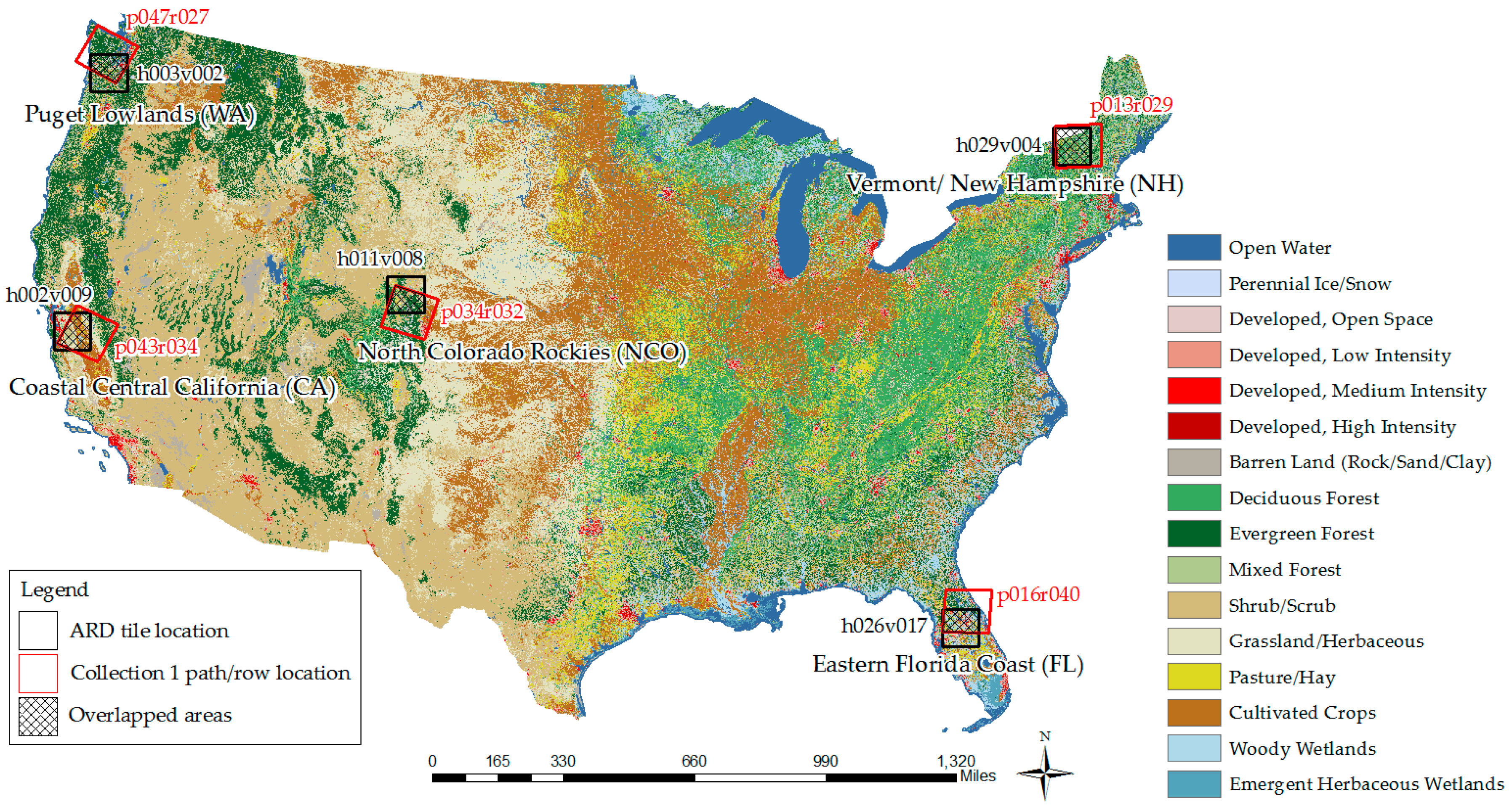
2.1. Study Sites

Five sites are selected over Conterminous U.S. (CONUS) in this study (Figure 1). The Vermont/New Hampshire (shortened as NH) site is dominated by different forests (e.g., deciduous, evergreen, and mixed forests) and the elevation gradient changes from sea level to 1914 m. The Puget Lowlands, Washington (shortened as WA) site is mainly characterized by frequent cloud covers and the great gradient variation changes from sea level to 4384 m. The Coastal Central California (shortened as CA) site is selected mostly for its complex agricultural practices, forest, and urban land covers, and the gradient variation changes from sea level to 3998 meters. The Northern Colorado Rockies (shortened as NCO) site is selected mainly due to the subtle elevation gradient ranging from 1406 to 3334 m (e.g., Rocky Mountain). The Eastern Florida Coast (shortened as FL) site is selected due to its urban landscape patterns and the elevation gradient changes from sea level to 152 m. Those sites are located at high, middle, and low latitudes respectively, so we will have Landsat observations from a wide range of solar zenith angles. Note that the topographic variations at each site were calculated based the corresponding Digital Elevation Model (DEM) data. The DEM data are from the Shuttle Radar Topography Mission (SRTM) one arc-second (approximately 30 meters) and were selected mainly considering of their relatively high overall accuracy [44].

2.2. Data

2.2.1. Landsat Collection 1

The Landsat Collection 1 data are provided for each WRS Path/Row, which is defined in Universal Transverse Mercator (UTM) projection referenced to the World Geodetic System 1984 (WGS84) datum. They are organized into Tier 1 (T1), Tier 2 (T2), and Real-Time (RT). The T1 and T2 data are processed based on a ground reference database (e.g., ground control points and pseudo-invariant calibration sites), while the RT data are only based on some estimated parameters. The T1 data can achieve relatively high geometric and radiometric quality as compared to T2 (except for T2 data from Landsat 8 which have similar accuracy as they are from T1). The RT image has the least quality and it will be replaced by T1 or T2 image once the corresponding ground references are available. In this study, we excluded all T2 images from Landsats 4–7 T2 and all RT images due to their relatively low geometry quality [20], and used the remaining Landsat Collection 1 images (Landsats 4–8 T1 and Landsat 8 T2) acquired between 1982 and 2017 in five study sites (Figure 1;

Table 1. Statistics of Landsat Analysis Ready Data (ARD) and Collection 1 data used in this study.

Location Name	ARD Images		Collection 1 Images
	Horizontal/Vertical Tile	# of Landsats 4–5/7/8	Path/Row Scene	# of Landsats 4–5/7/8
Coastal Central California (CA)	002/009	1283/1054/278	043/034	452/360/98
Eastern Florida Coast (FL)	016/040	1151/964/240	016/040	434/329/91
North Colorado Rockies (NCO)	034/032	1194/944/244	034/032	410/322/86
Vermont, New Hampshire (NH)	013/029	818/625/171	013/029	286/206/50
Puget Lowlands, Washington (WA)	047/027	971/752/245	047/027	263/177/56

). For each image, Surface Reflectance (SR) of six spectral bands, such as three visible bands (blue, green, and red), one near infrared (NIR) band, and two shortwave infrared bands (SWIR 1 and SWIR 2) were used in this study. Note that the SR products were provided by USGS Earth Resources Observation and Science (EROS) Center Science Processing Architecture (ESPA) (https://espa.cr.usgs.gov), in which Landsats 4–5 and 7 data were generated by the Landsat Ecosystem Disturbance Adaptive Processing System (LEDAPS) [46], and Landsat 8 data were generated by the Landsat Surface Reflectance Code (LaSRC) [16]. Except for the SR of the Collection 1 data, we also used the corresponding raw digital numbers (DN) images as the input for Fmask 4.0 algorithm.

2.2.2. Landsat ARD

The Landsat ARD are based on the same raw data for Landsats 4–8 Collection 1 T1 and Landsat 8 Collection 1 T2 imagery and are produced using the Landsat Collection 1 processes, except a different map projection (the Albers Equal Area Conic referenced to the WGS84 datum) is employed [22]. The Landsat ARD include Landsats 4–5 Thematic Mapper (TM), Landsat 7 Enhanced Thematic Mapper Plus (ETM+), and Landsat 8 Operational Land Imager (OLI)/Thermal Infrared Sensor (TIRS) imagery, which are provided with non-overlapping tiles of 5000 × 5000 30-m pixels (Horizontal/Vertical tile) [23]. Following the determined Landsat Collection 1 Path/Row scenes, we further selected the corresponding ARD tiles. As a Collection 1 Path/Row scene often consists of multiple ARD tiles, we only used the ARD tile that has a maximum overlapping area with each scene for simplicity. In each tile, all available Landsat ARD acquired between 1982 and 2017 with cloud cover less than 80% were used (Figure 1; Table 1). Note that the percentage of cloud cover was computed using the QA band generated by Fmask 3.3 [17,29]. For each image, the SR of six spectral bands corresponding to the Landsat Collection 1 data were used.

3. Methodologies

We designed four different scenarios for evaluating and improving the temporal consistency of LTS as follows: (1) build LTS based on ARD and compare it with same extent double-resampled Collection 1 data; (2) screen clouds and cloud shadows based on Fmask 4.0 and assess its effects on the LTS consistency as compared to Fmask 3.3; (3) correct the BRDF effects using the c-factor approach proposed by Roy et al. [33] to improve the LTS consistency; and (4) correct and evaluate the topographic effects on the LTS consistency using SCS, SCS + C, and IC algorithms. The detailed information on input data and processing methods for the four scenarios is listed in

Table 2. Different scenarios for evaluating and improving the consistency of LTS. The c-factor approach is proposed by Roy et al. [33]; SCS: Sun-Canopy-Sensor proposed by Gu et al. [40]; SCS+C: a semiempirical SCS proposed by Soenen et al. [41]; and, IC: Illumination Correction proposed by Tan et al. [42].

Scenario Number	Input Data	Methods
		Reprojection	Cloud/Cloud Shadow	BRDF Correction	Topographic Correction
1	Collection 1 vs. ARD from the Same Path/Row	Single vs. Double	Fmask 3.3	No	No
2	ARD from the Same Path/Row	Single	Fmask 3.3 vs. Fmask 4.0	No	No
3	All ARD	Single	Fmask 3.3	c-factor approach	No
4	All ARD	Single	Fmask 3.3	No	SCS, SCS+C, and IC

.

3.1. Reprojection of Landsat Collection 1 Data

Historically, Landsat data are provided at a spatial extent of 180 × 180 km for each Path/Row. Landsat Collection 1 data are provided in the same way and has been used extensively for time series analysis. However, before they are used for time series analysis, we need to re-project them into the same spatial extent and data dimension to make them comparable [9,47,48]. As we mentioned above, this process will involve two resampling procedures, but no longer necessary for Landsat ARD. To quantitatively demonstrate the LTS consistency based on ARD compared to Collection 1 data, we re-projected all Landsat Collection 1 images into the same extent as the corresponding Landsat ARD tile using the nearest neighbor resampling approach [49]. Additionally, we only used ARD and Collection 1 data acquired at the same time and from the same Landsat Path/Row. In this scenario, the same ARD QA band (generated by Fmask 3.3) was used to screen clouds and cloud shadows.

3.2. Screening Clouds and Cloud Shadows

The presence of clouds and cloud shadows can lead to sudden changes in reflectance and thus have severe effects on the consistency of LTS. Before most of the LTS-based applications, clouds and cloud shadows should be screened out as the first step [26,28,50]. At present, the QA band of Landsat ARD is generated mainly by using Fmask 3.3 [17,29]. However, the Fmask algorithm has gone through a major upgrade from version 3.3. to version 4.0 [31]. The 4.0 version has improved cloud and cloud shadow detection accuracy substantially by (1) integrating Global Surface Water Occurrence (GSWO) to better separate water and land; (2) integrating global DEM to normalize thermal and cirrus bands; (3) recalibrating new cloud probability thresholds for different sensors (e.g., TM, ETM+, and OLI/TIRS); (4) utilizing spectral-contextual features to reduce the misidentified clouds that are caused by bright and white surfaces (e.g., snow/ice and urban/built-up); and, (5) integrating DEM for better cloud shadow detection for mountainous areas [32]. In this study, we attempted to use the new Fmask 4.0 results to improve the LTS consistency. While considering that Fmask is a scene-based algorithm, we applied the Fmask 4.0 algorithm over the corresponding Collection 1 image to generate the new QA band and re-projected it into the same ARD tile. Finally, we can assess the LTS consistency for ARD controlled by Fmask 4.0 and Fmask 3.3 algorithms.

3.3. BRDF Correction

The BRDF effects of the ARD data were corrected using the c-factor approach [33] based on the RossThick-LiSparse-R BRDF model [35]. Directional reflectance can be normalized to nadir-view reflectance, as follows:

$$\check{\rho }=\rho ·\frac{f_{iso}+f_{vol}·K_{vol}\left(\theta \prime ,0°,0°\right)+f_{geo}·K_{geo}\left(\theta \prime ,0°,0°\right)}{f_{iso}+f_{vol}·K_{vol}\left(\theta ,\varnothing ,\phi \right)+f_{geo}·K_{geo}\left(\theta ,\varnothing ,\phi \right)}$$

(1)

where,

• $\varnothing$ is the view zenith angle,
• $\phi$ is the view-sun relative azimuth angle,
• $\theta$ is the solar zenith angle,
• $\theta \prime$ is the normalized solar zenith angle,
• $\rho$ is the original reflectance (directional reflectance),
• $\check{\rho }$ is the BRDF-normalized reflectance (nadir-view reflectance),
• $f_{iso}$, $f_{vol}$, and $f_{geo}$ are the parameters of the BRDF model [35],
• $K_{vol}\left(\theta ,\varnothing , \phi \right)$ is the RossThick kernel [51],
• $K_{geo}\left(\theta ,\varnothing ,\phi \right)$ is the LiSparse-R kernel [51].

A fixed set of BRDF spectral model parameters [33] were used for BRDF correction in this study. They were derived from more than 15 billion pixels over global MODIS 500-m BRDF parameters product [35]. When considering that the empirical BRDF parameters are not applicable for snow/ice pixels, we excluded all of the snow observations in this evaluation. According to the findings of Zhang et al. [52], the optimal normalized solar zenith angle (${\theta }^{\prime }$) was set constant per location, and it follows a sixth-degree polynomial as a function of the central latitude ($\eta$) of the image [53]:

$$\begin{array}{c}{\theta }^{\prime }=31.0076-0.1272\times \eta +0.01187\times {\eta }^2+2.4\times {10}^{-5}\times {\eta }^3-9.48\times {10}^{-7}\times {\eta }^4\\ -1.95\times {10}^9\times {\eta }^5+6.15\times {10}^{-11}\times {\eta }^6\end{array}$$

(2)

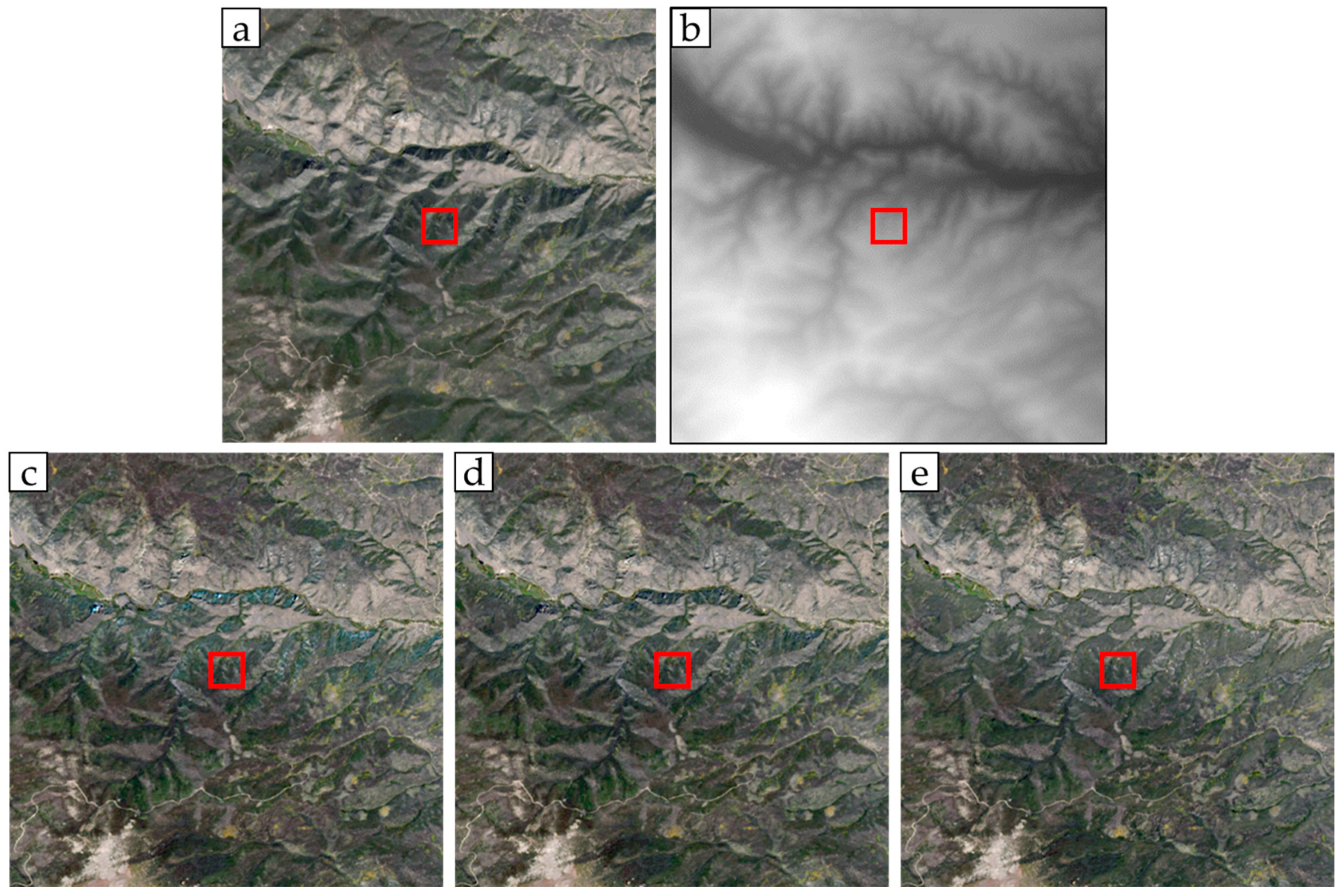
3.4. Topographic Correction

To comprehensively assess the topographic effect on the LTS consistency, we used three widely used models to remove the topographic effects in Landsat ARD, including SCS [40], SCS + C [41], and IC [42].

3.4.1. The SCS Model

The SCS correction is equivalent to projecting the sunlit canopy from the sloped surface to the horizontal surface in the direction of illumination [40]. It assumes that the geometric relationship between the sun and the tree canopy keeps the same before and after correction due to the geotropic (vertical) nature of tree growth. The integrated reflectance from the sunlit canopy is proportional to its area. The model is expressed, as follows:

$$\widehat{\rho }=\rho ·\frac{\cos (\theta )·\cos (\alpha )}{\cos (i)}$$

(3)

$$\cos i=\cos \left(\theta \right)·\cos (\alpha )+\sin (\theta )·\sin (\alpha )·\cos (\Omega -\beta )$$

(4)

where,

• $\widehat{\rho }$ is the topography-corrected reflectance,
• $\Omega$ is the solar azimuth angle,
• $\alpha$ is the slope angle,
  $\beta$ is the aspect angle of the slope, and
• $\cos i$ is the cosine of the local solar incidence angle ($i$) calculated by Equation (4).

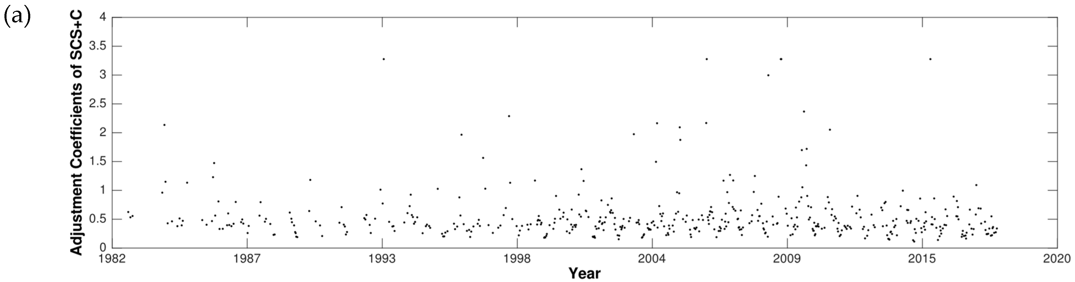
3.4.2. The SCS+C Model

The SCS+C model is based on the same SCS model, but it integrates a semi-empirical parameter (C) that can significantly reduce the overcorrection caused by the scattered radiation from the source of illumination [41]. The correction of SCS+C model is expressed, as follows:

$$\widehat{\rho }=\rho ·\frac{\cos (\theta )·\cos (\alpha ) +C}{\cos \left(i\right) +C}$$

(5)

where, C is an estimated parameter analogous to the effects of clear-sky irradiance [54].

The parameter C was proposed based on the assumption that there is a linear relationship between the uncorrected reflectance ($\rho$) and the cosine of the local solar incidence angle ($\cos i$) over clear-sky land pixels (Equation (6)), and it can be calculated by using the ratio of the intercept ($b$) and the slope ($a$) of the linear regression (Equation (7)) [54]. We applied a sampling approach stratified on the $\cos i$ with 0.1 increment to select a total of 40,000 clear-sky land pixels (based on Fmask 3.3 results) and estimated the slope ($a$) and the intercept ($b$) using the Ordinary Least Square (OLS) regression method [32].

$$\rho =a·\cos \left(i\right)+b$$

(6)

$$C=b/a$$

(7)

3.4.3. The IC Model

The IC model was proposed to remove the dependency of the reflectance on the cosine of the local solar incidence angle ($\cos i$) based on the same linear regression shown by Equations (6) and (7) [42]. It can be expressed, as follows:

$$\widehat{\rho }=\rho -a·\left(\cos \left(i\right)-\cos \left(i^{\prime }\right)\right)$$

(8)

where, $\cos i^{\prime }$ is the $\cos i$ for a horizontal surface calculated using Equation (4) with a slope angle (α) of 0.

As $\cos i$ is sensitive to land cover types, such as vegetation (e.g., forest) and non-vegetation type (e.g., soil and rock), the IC approach creates 3 × 3 km moving windows over the entire image and in each window it uses a threshold of 0.5 in Normalized Difference Vegetation Index (NDVI) to separate all pixels into a dense vegetation and a sparse vegetation group. In each group, a regression will be performed based on all clear-sky land pixels (Equation (6)).

3.5. Assessment of Temporal Consistency

Assume that there is no land surface change within a short period from date 1 (d1) to date 2 (d2), then the clear-sky SR at d1 and d2 should be very similar. Therefore, we use the SR difference between two consecutive observations within a short temporal period to indicate the temporal consistency of LTS. The smaller the difference, the better the consistency. The SR difference ($\Delta {\rho }_{d21}$) for each band between the two closest acquisition dates (d1 and d2) can be computed by $\Delta {\rho }_{d21}={\rho }_{d2}-{\rho }_{d1}$. In this study, we calculated the clear-sky SR differences within the entire LTS and limited the two closest acquisition dates within 16 days. Note that sometimes the intervals are eight days due to the combinations of two different Landsat satellites (e.g., Landsat 7 and Landsat 8), or even less in the overlapping areas [55].

The histogram of the SR differences for all pixels in an ARD tile was applied to evaluate the LTS consistency, and if the shape of the histogram is thin and tall, the consistency is high. At the same time, the Standard Deviation (SD) of SR difference was chosen to quantify the consistency of LTS. The smaller the SD, the better the consistency. Note that we only calculated the SD within the 95% confidence interval for topographic correction and BRDF correction. This is to exclude the effects of the missed clouds and cloud shadows in the Landsat QA band.

4. Results

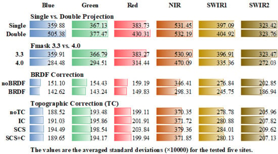
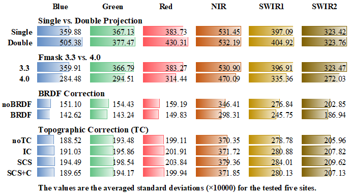
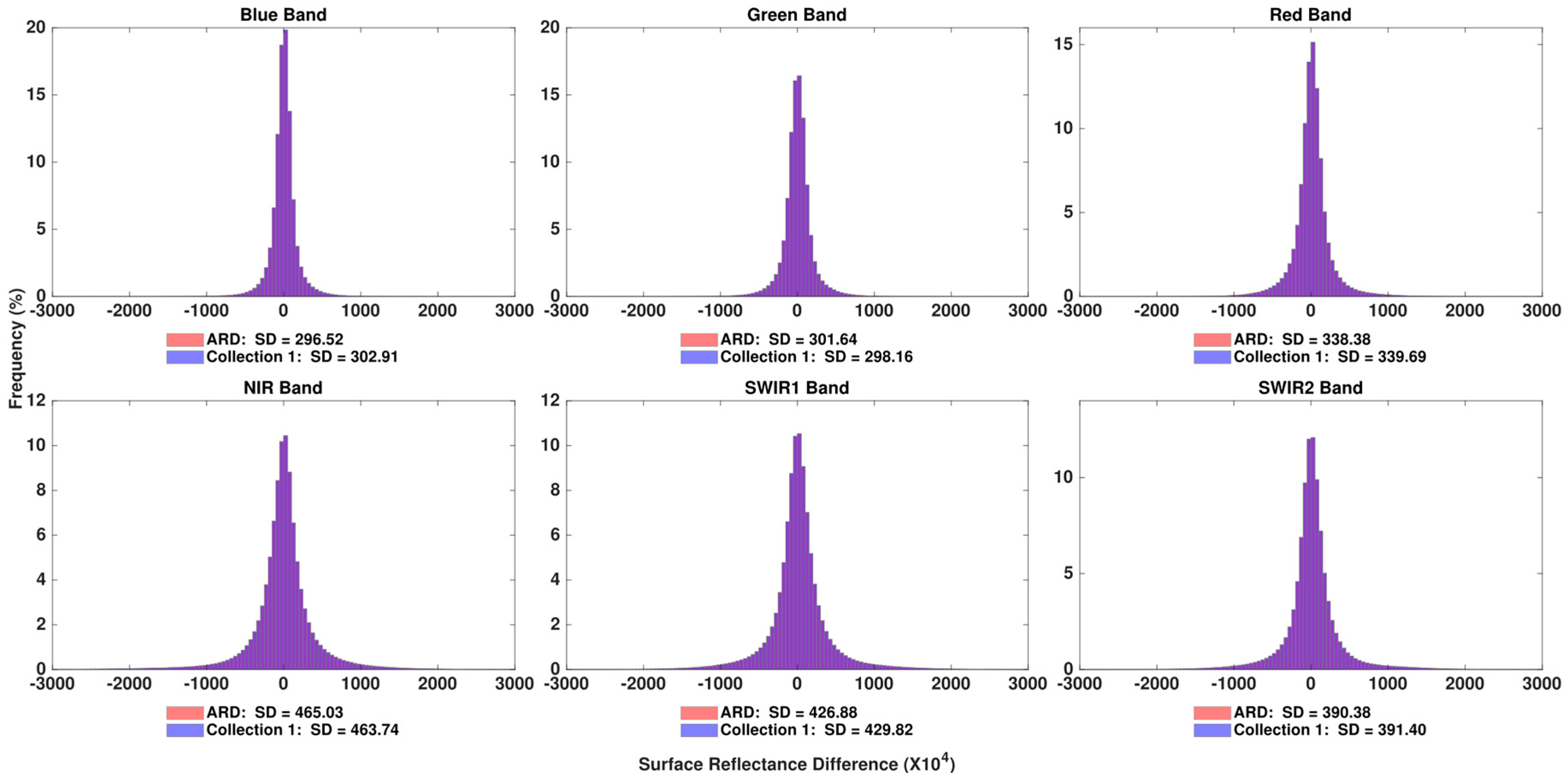
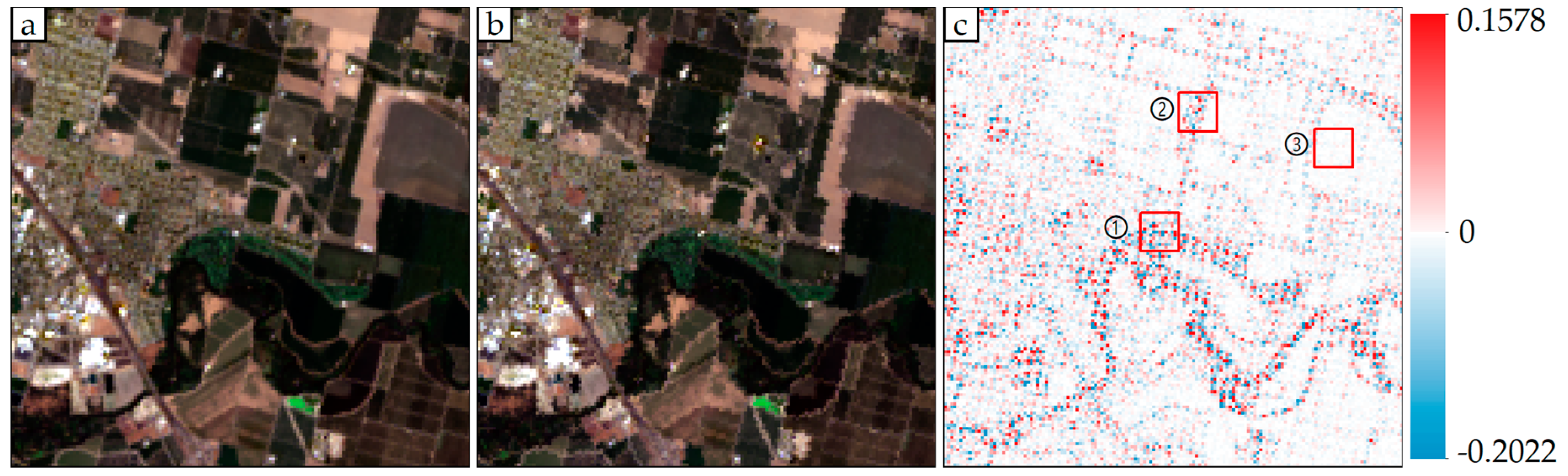
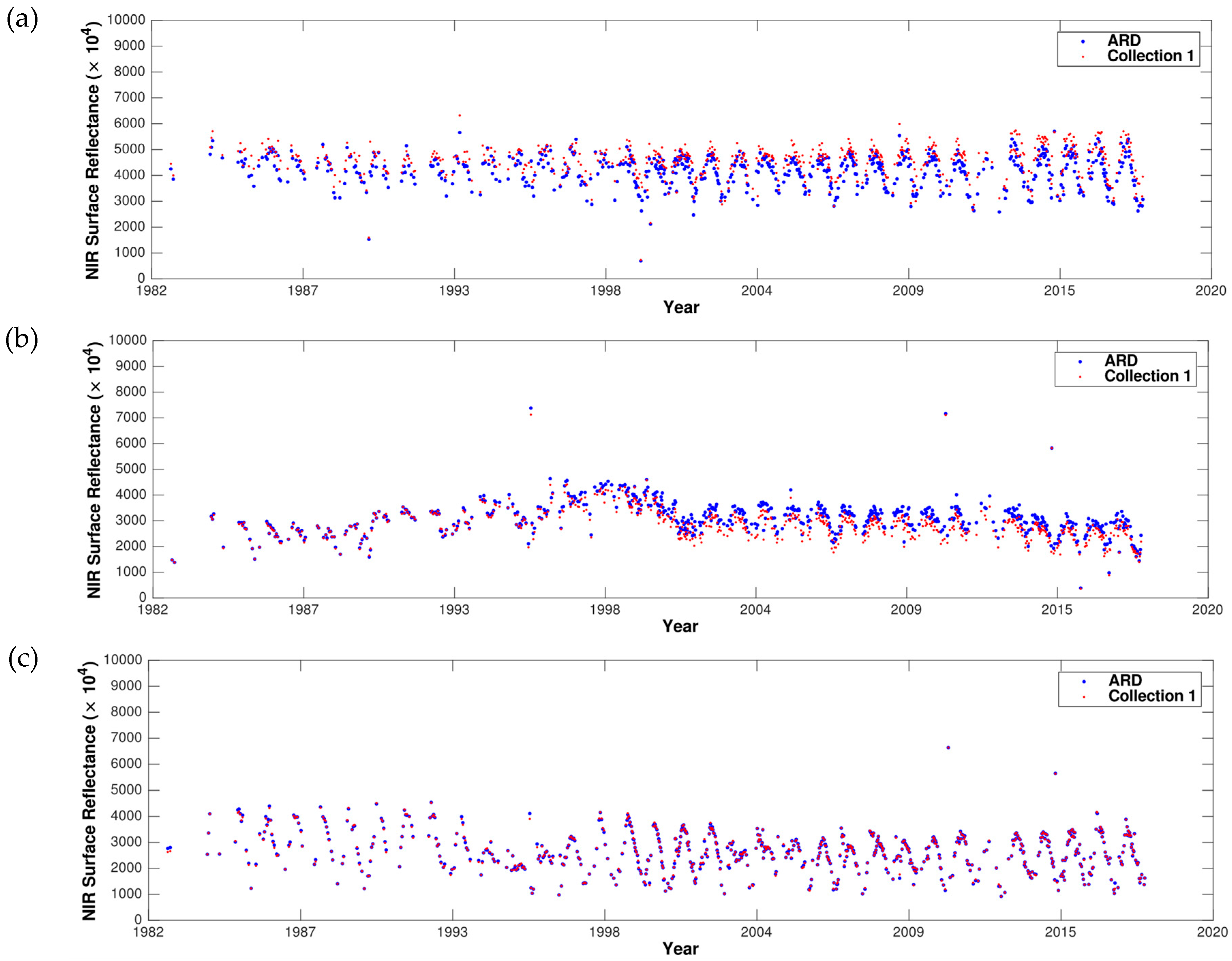
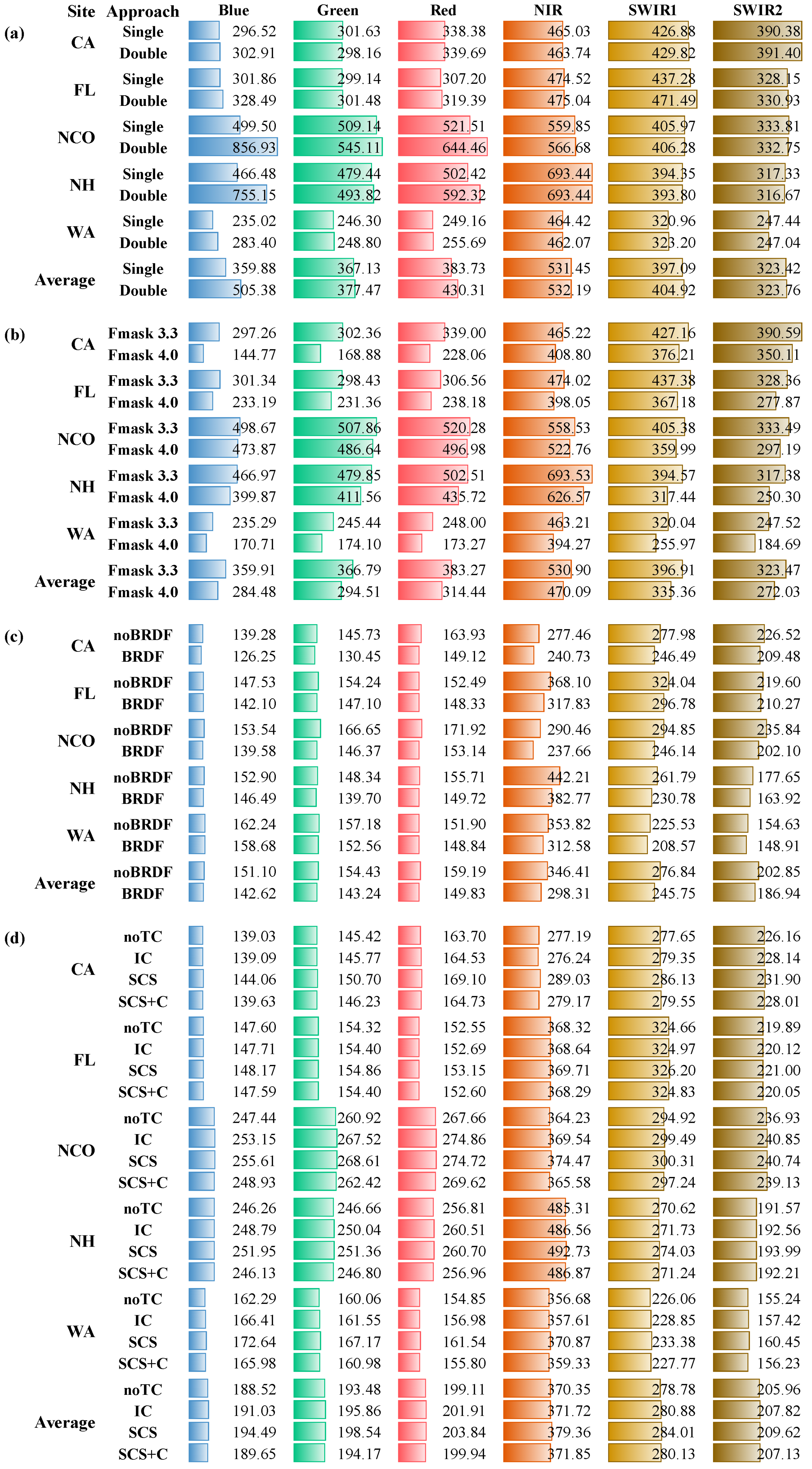
4.1. Scenario 1: The Influence of Single- (ARD) vs. Double-resampling (Collection 1) on LTS

Figure 2 shows the histograms of SR differences between ARD and Collection 1 data for each band at the CA site characterized by large areas of urban/built-up and agriculture. The distributions of the SR difference of ARD are very similar to that of Collection 1 data for all spectral bands, but ARD always achieved slightly lower SD when compared to the same measurements in Collection 1 data. This means that Landsat ARD and Collection 1 have similar data consistency, but ARD is slightly better than Collection 1 data. Similar results can be also found in Figure S1–S4 for the other four tested sites.

A comparison between ARD and Collection 1 image at the CA site is shown in Figure 3. While the two images are visually similar, ARD provide “smoother” landscape patterns than Collection 1 data (after the nearest neighbor resampling) (Figure 3). This is because the nearest neighbor resampling process will lead to pixel shifts and thus reduce geometric fidelity for Landsat Collection 1 data, particularly for the places with a large spatial difference, such as the pixels located at the boundaries of urban/built-up and crop fields (Figure 3c). This finding is also similar to that made by Dwyer et al. [22]. Additionally, the time series observations from ARD and Collection 1 data at locations 1–3 in Figure 3c showed that the ARD values can be systematically higher or lower than the Collection 1 at edge pixels (Figure 4a,b), but for pixels located at homogeneous places, such as the center of an agricultural field, they are almost the same (Figure 4c). Therefore, though the consistency between Collection 1 and ARD are very similar, ARD are preferred, as they preserve edge pixels values better and are easier to be applied in time series analysis.

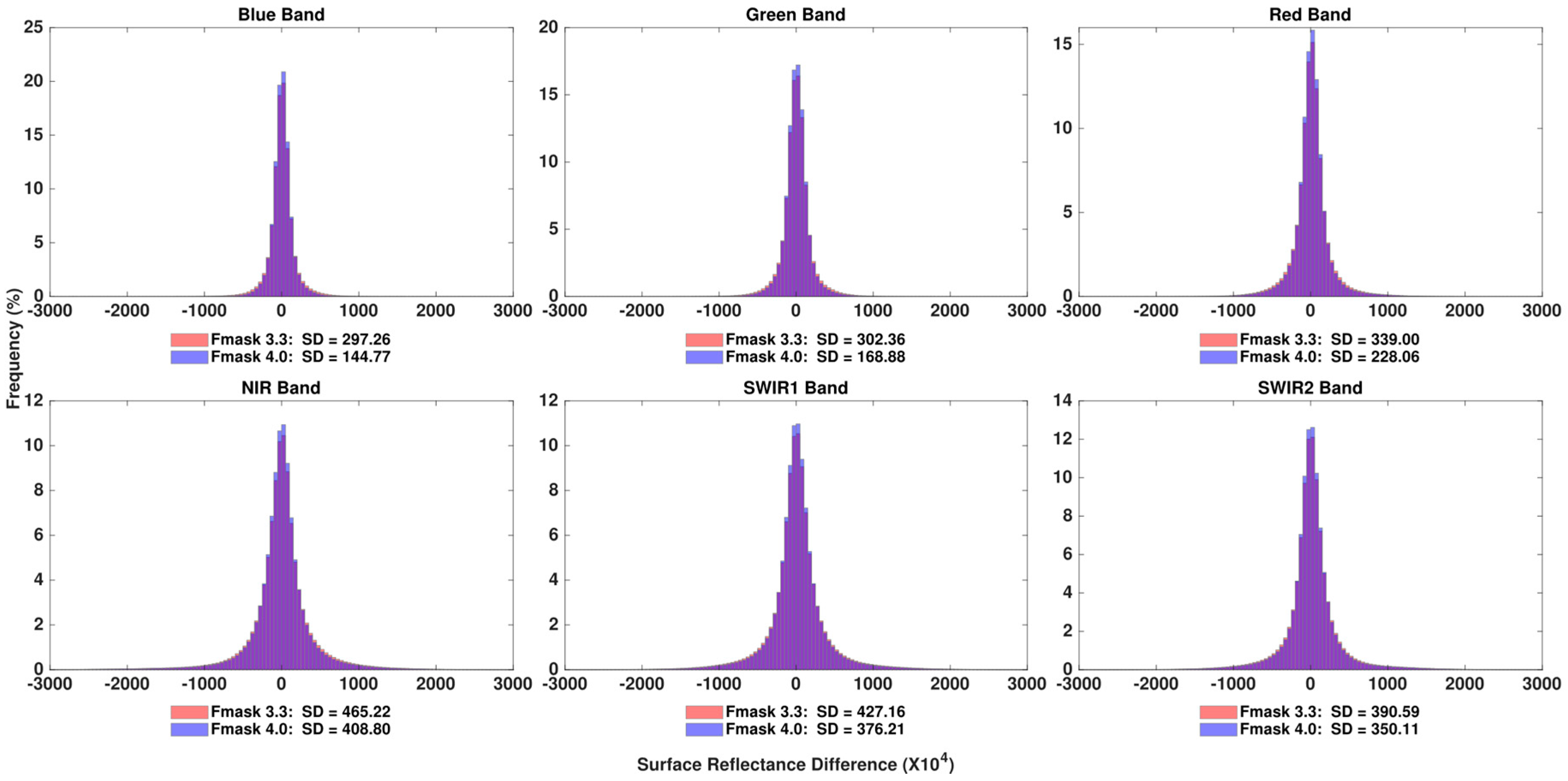
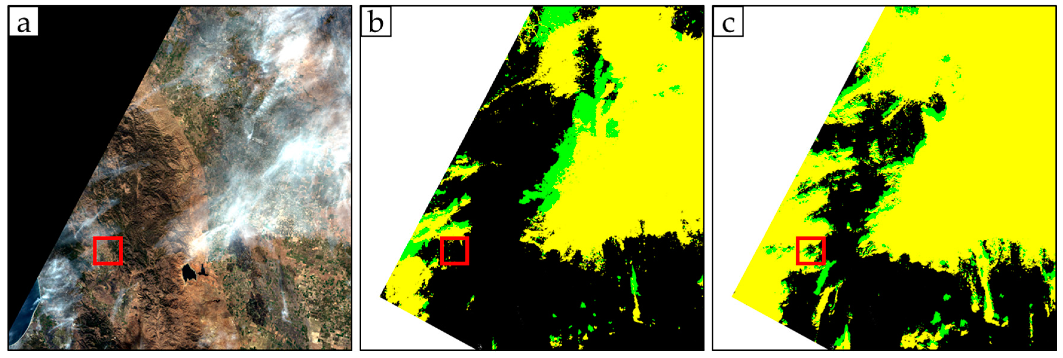
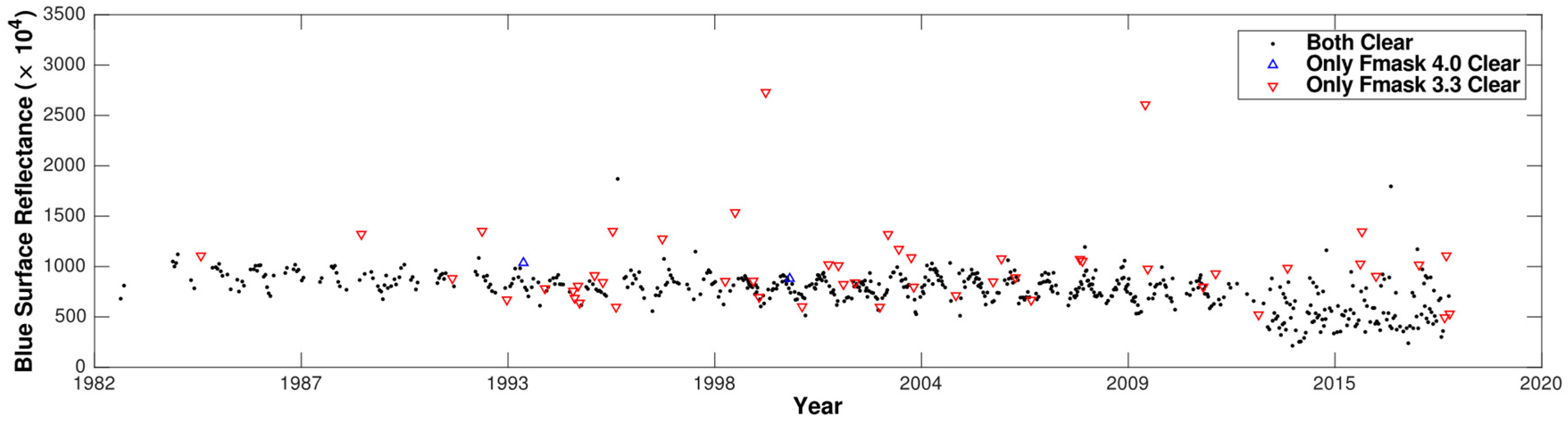
4.2. Scenario 2: The Influence of Improved Cloud and Cloud Shadow Detection Algorithm

We applied Fmask 4.0 algorithm for ARD from the same Path/Row and compared the influence of using a different version of Fmask (e.g., 3.3 version) on the consistency of LTS. As Figure 5 illustrates, Fmask 4.0 significantly reduced SDs when compared to Fmask 3.3 at the CA site. The same results were observed at other four test sites (Figure S5–S8). This suggests the LTS consistency are influenced substantially by clouds and cloud shadows, and a more accurate cloud and cloud shadow detection algorithm, such as Fmask 4.0, can be quite beneficial. Figure 6 illustrates a comparison between Fmask 4.0 and Fmask 3.3 for a Landsat 8 image. It shows Fmask 3.3 may fail to detect some clouds (especially thin clouds), but Fmask 4.0 succeeded. The missed clouds and cloud shadows from Fmask 3.3 would decrease the consistency of the entire LTS due to the sudden changes in SR (Figure 7). Therefore, the Fmask 4.0 algorithm is recommended to identify clouds and cloud shadows for LTS applications.

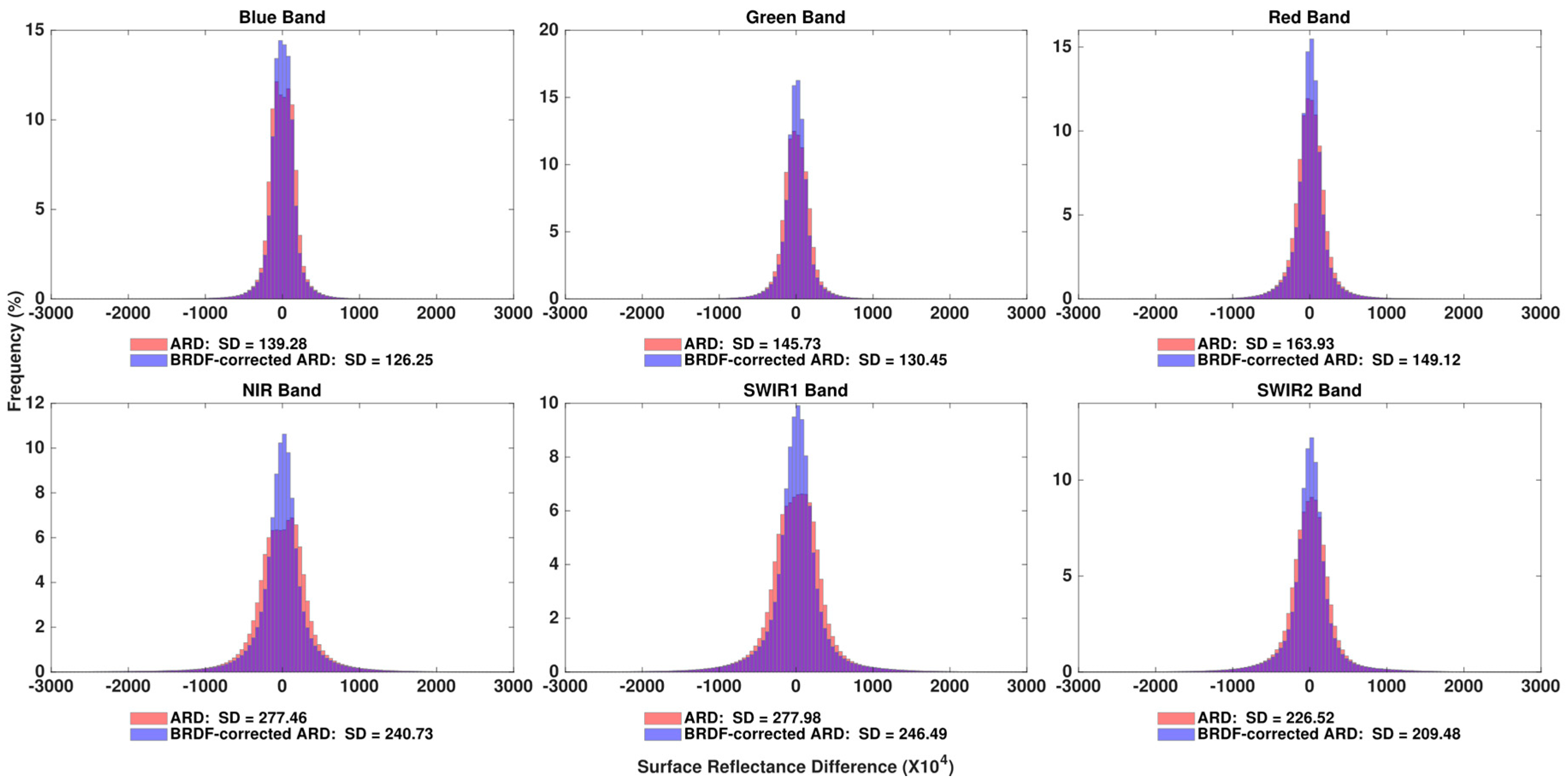
4.3. Scenario 3: The Influence of BRDF Correction

The BRDF correction was conducted to guarantee that every observation in the time series for a given pixel location was obtained at nadir view and for a fixed (latitudinally dependent) solar zenith. Figure 8 shows the histograms of SR difference between the original ARD and the BRDF-corrected ARD for different bands at the CA site. The SR difference of BRDF-corrected ARD shows a taller and thinner shape when compared to the original data. The histograms of visible bands are much thinner than the histograms of NIR and SWIR bands, which might be explained by the relatively low reflectance values of visible bands when compared to NIR and SWIR bands. Quantitative results demonstrated that the SDs of BRDF-corrected ARD are much smaller than that of the original ARD. The same results were also observed over other four test sites (Figure S9–S12). These results indicated that conducting BRDF correction is very important and necessary for improving the consistency of Landsat ARD.

The BRDF effects are more significant in the overlapped areas in Landsat ARD due to the large difference between surface reflectance observed in the forward and backward directions. Figure 9 shows the temporal distributions of the four solar and view angles for a pixel in the overlapped areas, including the forward and backward observations (e.g., view azimuth angles from 0° to 360° and view zenith angles from −7.5° to 7.5°). For both directions (Figure 9a,c), the solar zenith angles can range from 20° to 70°, while the solar azimuth angles can be different from 100° to 170°. For the sensor azimuth and zenith angles, there are two different distribution ranges that can be caused by the forward and backward observations. In the forward direction (Figure 9b), sensor zenith angles can range from 4.5° to 7°, while sensor azimuth angles can be different from −85° to −78° (a slight difference compared with the solar angles); in the backward direction (Figure 9d), sensor zenith angles can range from 7° to 7.5°, while sensor azimuth angles can be different from 100° to 112°. Each distribution range was relatively small, and this is one of the reasons why a fixed set of BRDF model parameters can be used for Landsat BRDF correction [33,56].

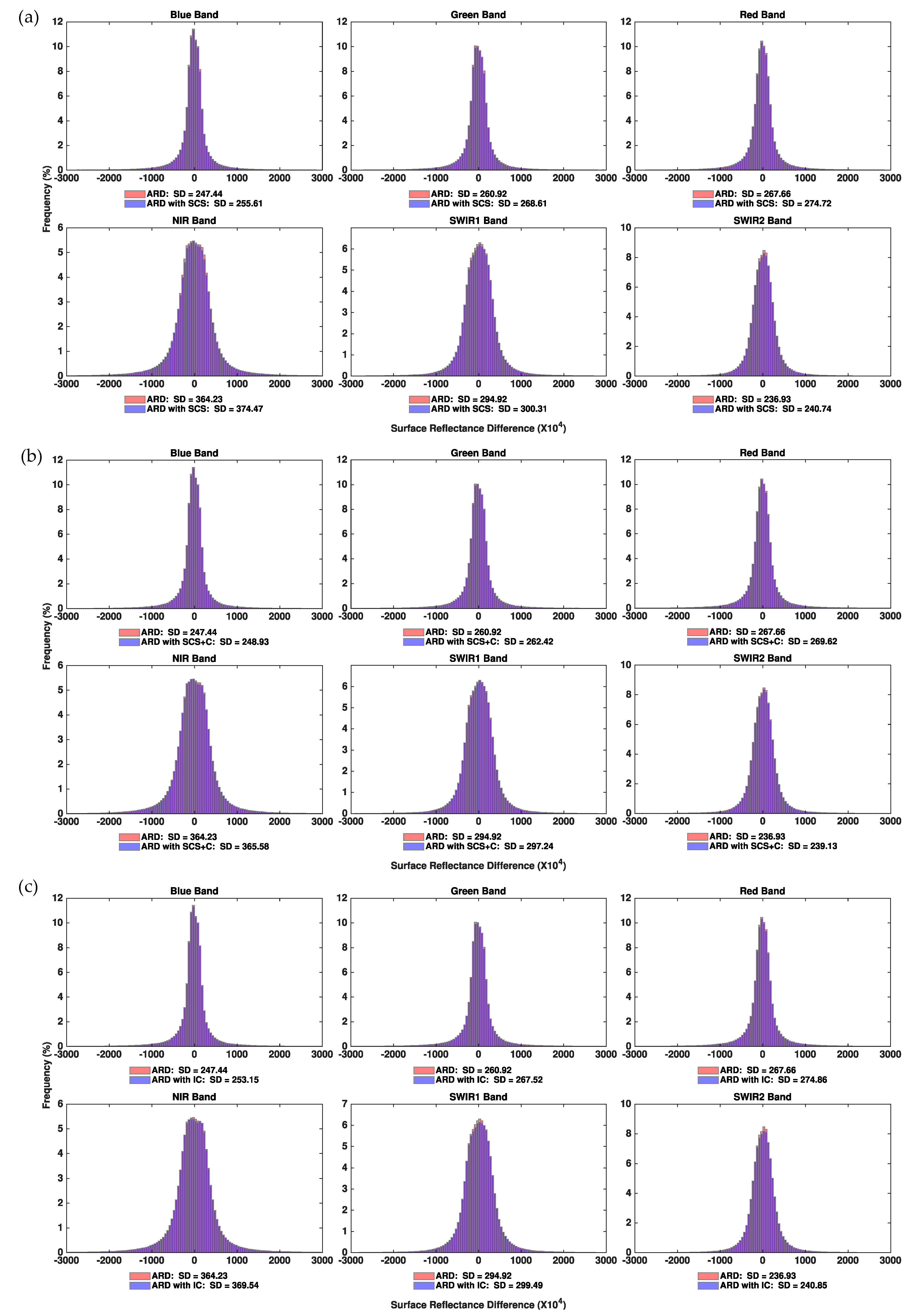
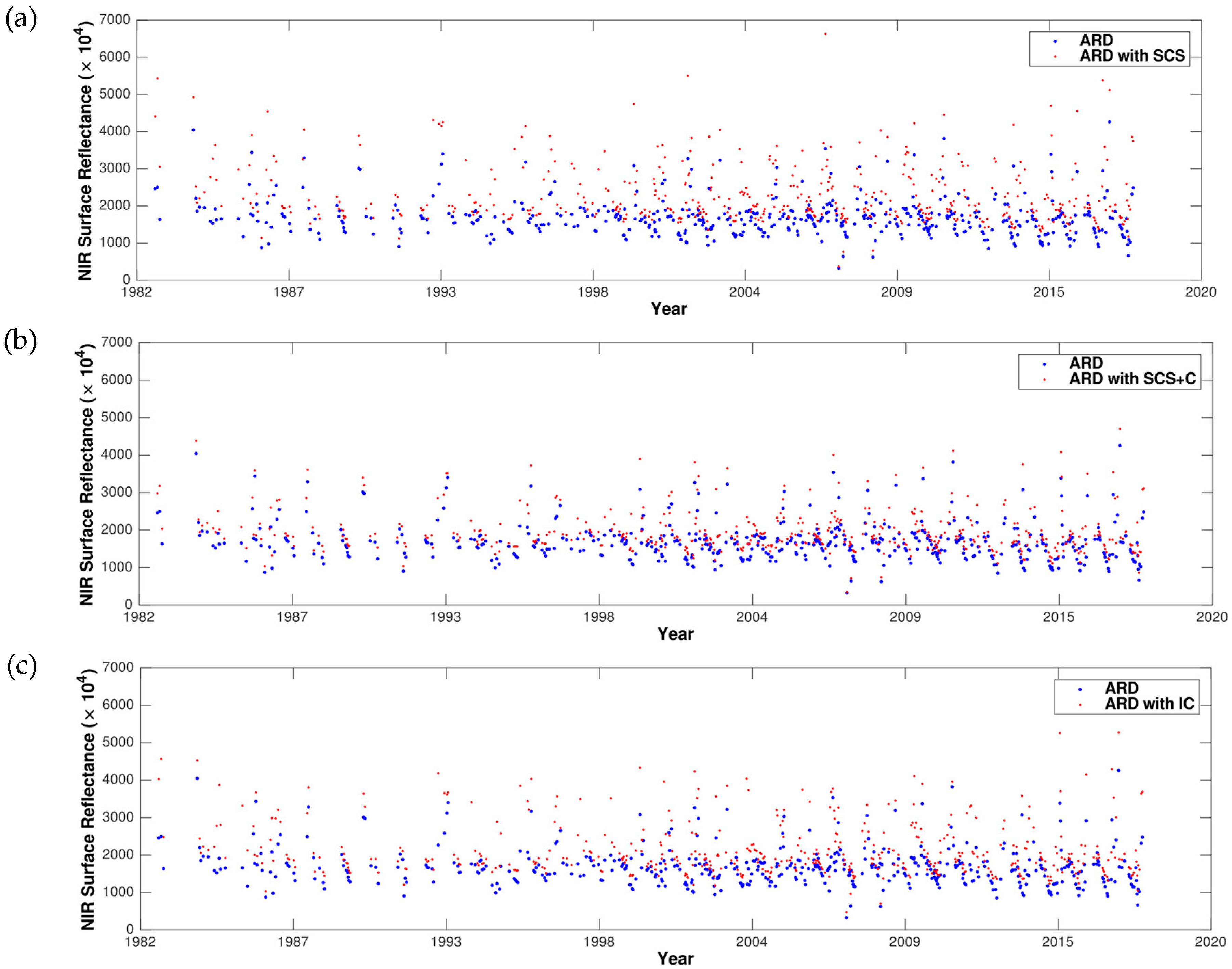
4.4. Scenario 4: The Influence of Topographic Correction

The topographic correction was conducted to reduce the terrain illumination effects. Figure 10 represents the histograms of comparisons between the original ARD surface reflectance and the topographic corrected ARD surface reflectance derived by SCS (Figure 10a), SCS+C (Figure 10b), and IC (Figure 10c) models for each band over the NCO site, where there are large topographic gradients. For each band, the histograms of the surface reflectance difference between the original data and the topographic corrected data shared almost the same shape. For the three topographic correction methods compared, the SD values of SCS+C and IC were almost the same and slightly larger than that from the original ARD. The SCS method showed relatively larger SD than the other two methods because of its overcorrection artifact [41]. The results showed that the three topographic correction methods did not contribute to improving the consistency of LTS in the NCO and similar results also were observed at other tested sites (Figure S13–S16).

Figure 11 illustrates the topographic corrected results derived by SCS (Figure 11c), SCS+C (Figure 11d), and IC (Figure 11e) for a Landsat ARD. Based on the visual comparison, the IC and SCS+C methods performed better, as the dark areas were often over-corrected by the SCS method. The same results can be observed from the SDs at different sites in Figure 10 and Figure S13–S16 (the SCS method generally has the largest SD value). At the same time, we also found that the SCS+C method generally has better performance than the IC method, especially for the three visible bands. However, the original ARD had the smallest SD value and showed better consistency than the topographically corrected time series. Figure 12 shows an example that the SCS, SCS+C, and IC method do not contribute on improving the consistency of a single Landsat pixel, in which the difference of adjacent observations is actually larger after the correction.

5. Discussion and Conclusions

Landsat ARD is a new dataset for facilitating time series analysis and the data consistency is one of the most important factors. This new data collect images from different sensors (e.g., TM, ETM+, and OLI/TIRS) and the consistency would be inherently effected [57,58]. Except for this effect, we explored four different scenarios (Table 2) for making LTS more consistent using Landsat ARD. In Figure 13, the color bars represent the magnitude of SD values for all spectral bands, five study sites, and four different testing scenarios, in which the shorter the bar, the more consistent the data.

First, we evaluated whether ARD (single-resampling) can result in a better consistency than Collection 1 (double-resampling). Results indicate that Landsat ARD has a slightly better consistency when compared to Landsat Collection 1 data (Figure 13a). This is mainly because each resampling process will lead to the loss of geometric fidelity, especially in places with a large spatial difference. In this study, we used the nearest neighbor resampling method to resample the Collection 1 data mainly because of its simple and fast characteristics, but it also resulted in pixel shifts that can make systematic biases and reduce the data consistency. Though other resampling methods, such as bilinear and cubic convolution, may provide better results than the nearest neighbor resampling method [59,60], they also change the value of samples by smoothing the data and generating artifacts at high contrast edges [24,61]. As the influenced pixels are relatively small (mostly edge pixels), there is very limited improvement in terms of data consistency between Collection 1 data and ARD. It is worth noting that the Landsat users may use or define other projection systems that are different from the current Landsat ARD projection, and we recommend using the Landsat ARD as it is for their analysis, and re-project the final results (e.g., classification or change detection maps) to their preferred map projections. Overall, the Landsat ARD are recommended to build LTS due to its slightly better consistency and easy-to-use.

Second, we demonstrated the benefit of using better cloud and cloud shadow detection algorithm (Fmask 3.3 vs. Fmask 4.0) for improving the consistency of LTS, and the improvement was substantial (Figure 13b). Considering that there are other more accurate cloud and cloud shadow detection algorithms that are based on multitemporal images, such as Tmask (multiTemporal mask), more consistent LTS is expected if they are applied [26,28]. However, it should be noted that the multitemporal cloud and cloud shadow detection algorithms may also remove some ephemeral surface changes, because they may have similar change patterns as clouds and cloud shadows [28].

Third, we assessed the impact of BRDF correction on the consistency of Landsat ARD. By using the c-factor approach with a fixed set of BRDF spectral model parameters [33], the consistency of Landsat ARD is significantly improved (Figure 13c). These parameters could be used for Landsat ARD, because the BRDF shapes of different terrestrial surfaces are sufficiently similar over the narrow 15° field of view [33,56], but they are not applicable to observations with large view angle variations or significant solar illumination variations [33]. In these cases, the local spatially and temporally contemporaneous BRDF model parameters are needed.

Last, none of the topographic correction methods that were tested in this study were helpful in improving LTS consistency (Figure 13d). The SCS topographic correction results showed large overcorrections. The results of SCS+C and IC were determined by the estimated parameters (Figure 14). The parameters were calculated either globally by the SCS+C method or locally by the IC method, and both methods can reduce overcorrection of dimly lit pixels effectively. The parameters of SCS+C fluctuated irregularly, because the clear observations used to fit the parameters were different on different dates. The parameters of IC fluctuated dramatically because the fitting process was retrieved for each 3 × 3 km moving window; however, for each ARD tile, there may not have enough valid observations to fill every moving window (e.g., pixels outside the scene boundary) to fit for the parameter in the IC method. Another reason may be that the topographic corrections were directly applied to the surface reflectance, which ignored the interactions between atmosphere and topography. In the future, the combination of atmospheric and topographic correction is encouraged to be tested for making the time series data more consistent. Finally, though the use of topographic correction may have limited contributions in improving temporal consistency, it can be beneficial for increasing the consistency of data in the spatial domain. For example, for land cover classification in mountainous areas, the use of the topographic corrected image can greatly reduce the classification errors in the shaded areas [62,63].

In conclusion, we evaluated and improved LTS consistency using Landsat ARD at five different sites in CONUS. The results suggest that (1) Landsat ARD are recommended to build LTS because the ARD data can achieve a slightly better time series consistency and are easier to use when compared to Landsat Collection 1 data. (2) LTS consistency can be further improved if a more accurate cloud and cloud shadow detection algorithm (e.g., Fmask 4.0) is used. (3) BRDF correction is the most important factor for improving the consistency of Landsat ARD. (4) Topographic corrections, such as SCS, SCS+C, and IC algorithms, generally have no contributions, and they may even reduce temporal consistency. These findings provide a routine guidance for how to build a consistent LTS for varies of LTS-based applications, such as forest disturbance, urban expansion, and agricultural practice.

References

1. Zhu, Z. Change detection using Landsat time series: A review of frequencies, preprocessing, algorithms, and applications. ISPRS J. Photogramm. Remote Sens. 2017, 130, 370–384. [Google Scholar] [CrossRef]
2. Kennedy, R.E.; Yang, Z.; Cohen, W.B. Detecting trends in forest disturbance and recovery using yearly Landsat time series: 1. LandTrendr—Temporal segmentation algorithms. Remote Sens. Environ. 2010, 114, 2897–2910. [Google Scholar] [CrossRef]
3. Huang, C.; Goward, S.N.; Masek, J.G.; Thomas, N.; Zhu, Z.; Vogelmann, J.E. An automated approach for reconstructing recent forest disturbance history using dense Landsat time series stacks. Remote Sens. Environ. 2010, 114, 183–198. [Google Scholar] [CrossRef]
4. DeVries, B.; Verbesselt, J.; Kooistra, L.; Herold, M. Robust monitoring of small-scale forest disturbances in a tropical montane forest using Landsat time series. Remote Sens. Environ. 2015, 161, 107–121. [Google Scholar] [CrossRef]
5. Pekel, J.-F.; Cottam, A.; Gorelick, N.; Belward, A.S. High-resolution mapping of global surface water and its long-term changes. Nature 2016, 540, 418–422. [Google Scholar] [CrossRef] [PubMed]
6. Tulbure, M.G.; Broich, M. Spatiotemporal dynamic of surface water bodies using Landsat time-series data from 1999 to 2011. ISPRS J. Photogramm. Remote Sens. 2013, 79, 44–52. [Google Scholar] [CrossRef]
7. Li, Y.; Zhang, H.; Kainz, W. Monitoring patterns of urban heat islands of the fast-growing Shanghai metropolis, China: Using time-series of Landsat TM/ETM+ data. Int. J. Appl. Earth Obs. Geoinf. 2012, 19, 127–138. [Google Scholar] [CrossRef]
8. Li, X.; Zhou, Y.; Zhu, Z.; Liang, L.; Yu, B.; Cao, W. Mapping annual urban dynamics (1985–2015) using time series of Landsat data. Remote Sens. Environ. 2018, 216, 674–683. [Google Scholar] [CrossRef]
9. Dara, A.; Baumann, M.; Kuemmerle, T.; Pflugmacher, D.; Rabe, A.; Griffiths, P.; Hölzel, N.; Kamp, J.; Freitag, M.; Hostert, P. Mapping the timing of cropland abandonment and recultivation in northern Kazakhstan using annual Landsat time series. Remote Sens. Environ. 2018, 213, 49–60. [Google Scholar] [CrossRef]
10. Yin, H.; Prishchepov, A.V.; Kuemmerle, T.; Bleyhl, B.; Buchner, J.; Radeloff, V.C. Mapping agricultural land abandonment from spatial and temporal segmentation of Landsat time series. Remote Sens. Environ. 2018, 210, 12–24. [Google Scholar] [CrossRef]
11. Woodcock, C.E.; Allen, R.; Anderson, M.; Belward, A.; Bindschadler, R.; Cohen, W.; Gao, F.; Goward, S.N.; Helder, D.; Helmer, E.; et al. Free Access to Landsat Imagery. Science 2008, 320, 1011a. [Google Scholar] [CrossRef] [PubMed]
12. Cohen, W.B.; Yang, Z.; Kennedy, R. Detecting trends in forest disturbance and recovery using yearly Landsat time series: 2. TimeSync—Tools for calibration and validation. Remote Sens. Environ. 2010, 114, 2911–2924. [Google Scholar] [CrossRef]
13. Hermosilla, T.; Wulder, M.A.; White, J.C.; Coops, N.C.; Hobart, G.W. An integrated Landsat time series protocol for change detection and generation of annual gap-free surface reflectance composites. Remote Sens. Environ. 2015, 158, 220–234. [Google Scholar] [CrossRef]
14. Lee, D.S.; Storey, J.C.; Choate, M.J.; Hayes, R.W. Four years of Landsat-7 on-orbit geometric calibration and performance. IEEE Trans. Geosci. Remote Sens. 2004, 42, 2786–2795. [Google Scholar] [CrossRef]
15. Mishra, N.; Helder, D.; Angal, A.; Choi, J.; Xiong, X. Absolute calibration of optical satellite sensors using Libya 4 pseudo-invariant calibration site. Remote Sens. 2014, 6, 1327–1346. [Google Scholar] [CrossRef]
16. Vermote, E.; Justice, C.; Claverie, M.; Franch, B. Preliminary analysis of the performance of the Landsat 8/OLI land surface reflectance product. Remote Sens. Environ. 2016, 185, 46–56. [Google Scholar] [CrossRef]
17. Zhu, Z.; Wang, S.; Woodcock, C.E. Improvement and expansion of the Fmask algorithm: Cloud, cloud shadow, and snow detection for Landsats 4-7, 8, and Sentinel 2 images. Remote Sens. Environ. 2015, 159, 269–277. [Google Scholar] [CrossRef]
18. Huang, C.; Goward, S.N.; Masek, J.G.; Gao, F.; Vermote, E.F.; Thomas, N.; Schleeweis, K.; Kennedy, R.E.; Zhu, Z.; Eidenshink, J.C.; et al. Development of time series stacks of Landsat images for reconstructing forest disturbance history. Int. J. Digit. Earth 2009, 2, 195–218. [Google Scholar] [CrossRef] [Green Version]
19. Roy, D.P.; Ju, J.; Kline, K.; Scaramuzza, P.L.; Kovalskyy, V.; Hansen, M.; Loveland, T.R.; Vermote, E.; Zhang, C. Web-enabled Landsat Data (WELD)—Landsat ETM+ composited mosaics of the conterminous United States. Remote Sens. Environ. 2010, 114ID–5, 35–49. [Google Scholar] [CrossRef]
20. USGS. Landsat Collection 1 Level 1 Product Definition. 2017. Available online: https://landsat.usgs.gov/sites/default/files/documents/LSDS-1656_Landsat_Level-1_Product_Collection_Definition.pdf (accessed on 18 December 2018).
21. Zhang, H.K.; Roy, D.P. Landsat 5 Thematic Mapper reflectance and NDVI 27-year time series inconsistencies due to satellite orbit change. Remote Sens. Environ. 2016, 186, 217–233. [Google Scholar] [CrossRef]
22. Dwyer, J.; Roy, D.; Sauer, B.; Jenkerson, C.; Zhang, H.; Lymburner, L. Analysis Ready Data: Enabling Analysis of the Landsat Archive. Remote Sens. 2018, 10, 1363. [Google Scholar] [CrossRef]
23. Egorov, A.V.; Roy, D.P.; Zhang, H.K.; Hansen, M.C.; Kommareddy, A. Demonstration of percent tree cover mapping using Landsat Analysis Ready Data (ARD) and sensitivity with respect to Landsat ARD processing level. Remote Sens. 2018, 10, 209. [Google Scholar] [CrossRef]
24. Li, Z.; Zhang, H.K.; Roy, D.P.; Yan, L.; Haiyan, H.; Jian, L. Landsat 15-m Panchromatic-Assisted Downscaling (LPAD) of the 30-m Reflective Wavelength Bands to Sentinel-2 20-m Resolution. Remote Sens. 2017, 9, 755. [Google Scholar] [CrossRef]
25. Mather, P.M.; Koch, M. Computer Processing of Remotely-Sensed Images: An Introduction; John Wiley & Sons: Hoboken, NJ, USA, 2011; ISBN 1119956404. [Google Scholar]
26. Zhu, Z.; Qiu, S.; He, B.; Deng, C. Cloud and cloud shadow detection for Landsat images: The fundamental basis for analyzing Landsat time series. In Remote Sensing Time Series Image Processing; CRC Press: Boca Raton, FL, USA, 2018; pp. 3–24. [Google Scholar] [CrossRef]
27. Huang, C.; Thomas, N.; Goward, S.N.; Masek, J.G.; Zhu, Z.; Townshend, J.R.G.; Vogelmann, J.E. Automated masking of cloud and cloud shadow for forest change analysis using Landsat images. Int. J. Remote Sens. 2010, 31, 5449–5464. [Google Scholar] [CrossRef]
28. Zhu, Z.; Woodcock, C.E. Automated cloud, cloud shadow, and snow detection in multitemporal Landsat data: An algorithm designed specifically for monitoring land cover change. Remote Sens. Environ. 2014, 152, 217–234. [Google Scholar] [CrossRef]
29. Zhu, Z.; Woodcock, C.E. Object-based cloud and cloud shadow detection in Landsat imagery. Remote Sens. Environ. 2012, 118, 83–94. [Google Scholar] [CrossRef]
30. Foga, S.; Scaramuzza, P.L.; Guo, S.; Zhu, Z.; Dilley, R.D.; Beckmann, T.; Schmidt, G.L.; Dwyer, J.L.; Joseph Hughes, M.; Laue, B. Cloud detection algorithm comparison and validation for operational Landsat data products. Remote Sens. Environ. 2017, 194, 379–390. [Google Scholar] [CrossRef] [Green Version]
31. Qiu, S.; Zhu, Z.; He, B. Fmask 4.0: Improved cloud and cloud shadow detection in Landsats 4-8 and Sentinel-2 imagery. Remote Sens. Environ. 2018. in review. [Google Scholar]
32. Qiu, S.; He, B.; Zhu, Z.; Liao, Z.; Quan, X. Improving Fmask cloud and cloud shadow detection in mountainous area for Landsats 4–8 images. Remote Sens. Environ. 2017, 199, 107–119. [Google Scholar] [CrossRef]
33. Roy, D.P.; Zhang, H.K.; Ju, J.; Gomez-Dans, J.L.; Lewis, P.E.; Schaaf, C.B.; Sun, Q.; Li, J.; Huang, H.; Kovalskyy, V. A general method to normalize Landsat reflectance data to nadir BRDF adjusted reflectance. Remote Sens. Environ. 2016, 176, 255–271. [Google Scholar] [CrossRef]
34. Lucht, W.; Schaaf, C.B.; Strahler, A.H. An algorithm for the retrieval of albedo from space using semiempirical BRDF models. IEEE Trans. Geosci. Remote Sens. 2000, 38, 977–998. [Google Scholar] [CrossRef]
35. Schaaf, C.B.; Gao, F.; Strahler, A.H.; Lucht, W.; Li, X.; Tsang, T.; Strugnell, N.C.; Zhang, X.; Jin, Y.; Muller, J.P.; et al. First operational BRDF, albedo nadir reflectance products from MODIS. Remote Sens. Environ. 2002, 83, 135–148. [Google Scholar] [CrossRef] [Green Version]
36. Roy, D.P.; Ju, J.; Lewis, P.; Schaaf, C.; Gao, F.; Hansen, M.; Lindquist, E. Multi-temporal MODIS-Landsat data fusion for relative radiometric normalization, gap filling, and prediction of Landsat data. Remote Sens. Environ. 2008, 112, 3112–3130. [Google Scholar] [CrossRef]
37. Gao, F.; He, T.; Masek, J.G.; Shuai, Y.; Schaaf, C.B.; Wang, Z. Angular effects and correction for medium resolution sensors to support crop monitoring. IEEE J. Sel. Top. Appl. Earth Obs. Remote Sens. 2014, 7, 4480–4489. [Google Scholar] [CrossRef]
38. Flood, N. Testing the local applicability of MODIS BRDF parameters for correcting Landsat TM imagery. Remote Sens. Lett. 2013, 4, 793–802. [Google Scholar] [CrossRef]
39. Justice, C.O.; Townshend, J.R.G.; Vermote, E.F.; Masuoka, E.; Wolfe, R.E.; Saleous, N.; Roy, D.P.; Morisette, J.T. An overview of MODIS Land data processing and product status. Remote Sens. Environ. 2002, 83, 3–15. [Google Scholar] [CrossRef] [Green Version]
40. Gu, D.; Gillespie, A. Topographic normalization of Landsat TM images of forest based on subpixel Sun-canopy-sensor geometry. Remote Sens. Environ. 1998, 64, 166–175. [Google Scholar] [CrossRef]
41. Soenen, S.A.; Peddle, D.R.; Coburn, C.A. SCS+C: A modified Sun-canopy-sensor topographic correction in forested terrain. IEEE Trans. Geosci. Remote Sens. 2005, 43, 2148–2159. [Google Scholar] [CrossRef]
42. Tan, B.; Masek, J.G.; Wolfe, R.; Gao, F.; Huang, C.; Vermote, E.F.; Sexton, J.O.; Ederer, G. Improved forest change detection with terrain illumination corrected Landsat images. Remote Sens. Environ. 2013, 136, 469–483. [Google Scholar] [CrossRef]
43. Chance, C.M.; Hermosilla, T.; Coops, N.C.; Wulder, M.A.; White, J.C. Effect of topographic correction on forest change detection using spectral trend analysis of Landsat pixel-based composites. Int. J. Appl. Earth Obs. Geoinf. 2016, 44, 186–194. [Google Scholar] [CrossRef]
44. Hirt, C.; Filmer, M.S.; Featherstone, W.E. Comparison and validation of the recent freely available ASTER-GDEM ver1, SRTM ver4. 1 and GEODATA DEM-9S ver3 digital elevation models over Australia. Aust. J. Earth Sci. 2010, 57, 337–347. [Google Scholar] [CrossRef]
45. Homer, C.H.; Fry, J.A.; Barnes, C.A. The National Land Cover Database; U.S. Geological Survey Fact Sheet 3020; U.S. Geological Survey Earth Resources Observation and Science (EROS) Center: Sioux Falls, SD, USA, 2012; pp. 1–4.
46. Masek, J.G.; Vermote, E.F.; Saleous, N.E.; Wolfe, R.; Hall, F.G.; Huemmrich, K.F.; Gao, F.; Kutler, J.; Lim, T. A Landsat Surface Reflectance Dataset. IEEE Geosci. Remote Sens. Lett. 2006, 3, 68–72. [Google Scholar] [CrossRef]
47. Hermosilla, T.; Wulder, M.A.; White, J.C.; Coops, N.C.; Hobart, G.W. Disturbance-Informed Annual Land Cover Classification Maps of Canada’s Forested Ecosystems for a 29-Year Landsat Time Series. Can. J. Remote Sens. 2018, 44, 67–87. [Google Scholar] [CrossRef]
48. Zhu, Z.; Woodcock, C.E.; Olofsson, P. Continuous monitoring of forest disturbance using all available Landsat imagery. Remote Sens. Environ. 2012, 122, 75–91. [Google Scholar] [CrossRef]
49. Tucker, C.J.; Compton, J.; Grant, D.M.; Dykstra, J.D. NASA’s Global Orthorectified Landsat data set. Am. Soc. Photogramm. Remote Sens. 2004, 70, 313–322. [Google Scholar] [CrossRef]
50. Zhu, X.; Helmer, E.H. An automatic method for screening clouds and cloud shadows in optical satellite image time series in cloudy regions. Remote Sens. Environ. 2018, 214, 135–153. [Google Scholar] [CrossRef]
51. Wanner, W.; Li, X.; Strahler, A.H. On the derivation of kernels for kernel-driven models of bidirectional reflectance. J. Geophys. Res. Atmos. 1995, 100, 21077–21089. [Google Scholar] [CrossRef]
52. Zhang, H.K.; Roy, D.P.; Kovalskyy, V. Optimal Solar Geometry Definition for Global Long-Term Landsat Time-Series Bidirectional Reflectance Normalization. IEEE Trans. Geosci. Remote Sens. 2016, 54, 1410–1418. [Google Scholar] [CrossRef]
53. Claverie, M.; Ju, J.; Masek, J.G.; Dungan, J.L.; Vermote, E.F.; Roger, J.-C.; Skakun, S.V.; Justice, C. The Harmonized Landsat and Sentinel-2 surface reflectance data set. Remote Sens. Environ. 2018, 219, 145–161. [Google Scholar] [CrossRef]
54. Teillet, P.M.; Guindon, B.; Goodenough, D.G. On the slope-aspect correction of multispectral scanner data. Can. J. Remote Sens. 1982, 8, 84–106. [Google Scholar] [CrossRef]
55. Roy, D.P.; Kovalskyy, V.; Zhang, H.K.; Vermote, E.F.; Yan, L.; Kumar, S.S.; Egorov, A. Characterization of Landsat-7 to Landsat-8 reflective wavelength and normalized difference vegetation index continuity. Remote Sens. Environ. 2016, 185, 57–70. [Google Scholar] [CrossRef]
56. Flood, N.; Danaher, T.; Gill, T.; Gillingham, S. An operational scheme for deriving standardised surface reflectance from Landsat TM/ETM+ and SPOT HRG imagery for eastern Australia. Remote Sens. 2013, 5, 83–109. [Google Scholar] [CrossRef]
57. Zhu, Z.; Fu, Y.; Woodcock, C.E.; Olofsson, P.; Vogelmann, J.E.; Holden, C.; Wang, M.; Dai, S.; Yu, Y. Including land cover change in analysis of greenness trends using all available Landsat 5, 7, and 8 images: A case study from Guangzhou, China (2000–2014). Remote Sens. Environ. 2016, 185, 243–257. [Google Scholar] [CrossRef]
58. Holden, C.E.; Woodcock, C.E. An analysis of Landsat 7 and Landsat 8 underflight data and the implications for time series investigations. Remote Sens. Environ. 2016, 185, 16–36. [Google Scholar] [CrossRef]
59. Gao, F.; Masek, J.G.; Wolfe, R.E. Automated registration and orthorectification package for Landsat and Landsat-like data processing. J. Appl. Remote Sens. 2009, 3, 033515. [Google Scholar] [CrossRef]
60. Parker, J.A.; Kenyon, R.V.; Troxel, D.E. Comparison of Interpolating Methods for Image Resampling. IEEE Trans. Med. Imaging 1983, 2, 31–39. [Google Scholar] [CrossRef] [PubMed]
61. Shlien, S. Geometric correction, registration, and resampling of Landsat imagery. Can. J. Remote Sens. 1979, 5, 74–89. [Google Scholar] [CrossRef]
62. Meyer, P.; Itten, K.I.; Kellenberger, T.; Sandmeier, S.; Sandmeier, R. Radiometric corrections of topographically induced effects on Landsat TM data in an alpine environment. ISPRS J. Photogramm. Remote Sens. 1993, 48, 17–28. [Google Scholar] [CrossRef]
63. Allen, T.R. Topographic normalization of Landsat thematic mapper data in three mountain environments. Geocarto Int. 2000, 15, 15–22. [Google Scholar] [CrossRef]
Figure 1. Five test sites. The background land cover is mapped from the 2011 National Land Cover Dataset (NLCD) [45].
Remotesensing 11 00051 g001
Figure 2. The histograms of SR difference between ARD and Collection 1 data based on a total of 9.14 billion SR difference values at the CA site. SD: Standard Deviation; SR: Surface Reflectance.
Remotesensing 11 00051 g002
Figure 3. A comparison between Landsat ARD and the corresponding Landsat Collection 1 image acquired on June 28, 2013 at the CA site (150 × 150 pixels). (a) True color Landsat ARD (red, green, and blue bands). (b) True color Landsat Collection 1 image (red, green, and blue bands). (c) The difference of near-infrared (NIR) band surface reflectance between ARD and Collection 1. The red squares 1–3 are the locations of example pixels in Figure 4a–c, respectively.
Remotesensing 11 00051 g003
Figure 4. Time series plot of near infrared (NIR) band surface reflectance over (a) an urban/built-up pixel located at the center of the red square 1 in Figure 3c, (b) a cropland edge pixel located at the center of the red square 2 in Figure 3c, and (c) a cropland pixel located at the center of the red square 3 in Figure 3c.
Remotesensing 11 00051 g004
Figure 5. The histograms of SR difference values between ARD with Fmask 3.3 (derived from 9.14 billion SR difference pixels) and that with Fmask 4.0 (derived from 8.46 billion SR difference pixels) at the CA site. SD: Standard Deviation; SR: Surface Reflectance.
Remotesensing 11 00051 g005
Figure 6. Comparison of cloud (yellow) and cloud shadow (green) detection results between Fmask 4.0 and Fmask 3.3 for a Landsat ARD acquired on November 3, 2013 at the CA site (5000 × 5000 pixels). (a) True color composite Landsat ARD (red, green, and blue bands). (b) Fmask 3.3 results. (c) Fmask 4.0 results. Note that Fmask 4.0 results were calculated based on the corresponding Landsat 8 Collection 1 data and re-projected into the same extent of Landsat ARD.
Remotesensing 11 00051 g006
Figure 7. Time series observations in blue band screened by Fmask 4.0 and Fmask 3.3 for a pixel located at the center of the red square in Figure 6 (urban/built-up). “Both clear” indicates the observations which are labeled as clear by Fmask 4.0 and Fmask 3.3 at the same time. “Only Fmask 4.0 clear” indicates the observations that Fmask 4.0 identified as clear, but Fmask 3.3 identified as cloud or cloud shadow. “Only Fmask 3.3 clear” indicates the observations that Fmask 3.3 identified as clear but Fmask 4.0 identified as cloud or cloud shadow.
Remotesensing 11 00051 g007
Figure 8. The histograms of SR difference values between original ARD and BRDF-corrected ARD based on a total of 4.21 billion SR difference pixels at the CA site. SD: Standard Deviation; SR: Surface Reflectance.
Remotesensing 11 00051 g008
Figure 9. Solar and sensor angles of the continuous observations in the forward and backward direction at a pixel in the CA site. (a) Solar azimuth and zenith angles in the forward direction. (b) Sensor azimuth and zenith angles in the forward direction. (c) Solar azimuth and zenith angles in the backward direction. (d) Sensor azimuth and zenith angles in the backward direction.
Remotesensing 11 00051 g009
Figure 10. The histograms of SR difference values between the topographically corrected ARD surface reflectance and original ARD surface reflectance derived from three different methods based on a total of 2.59 billion SR difference values at the NCO site. From the top to bottom are the (a) SCS, (b) SCS+C, (c) IC. SD: Standard Deviation; SR: Surface Reflectance; SCS: Sun-Canopy-Sensor; SCS+C: a semiempirical SCS; IC: Illumination Correction.
Remotesensing 11 00051 g010
Figure 11. Topographically corrected results for a subset Landsat ARD acquired on June 19, 2015 at the NCO site (300 × 300 pixels). (a) True color image (red, green, and blue bands). (b) DEM. (c) SCS result. (d) SCS+C result. (e) IC result. DEM: Digital Elevation Model; SCS: Sun-Canopy-Sensor; SCS+C: a semiempirical SCS; IC: Illumination Correction.
Remotesensing 11 00051 g011
Figure 12. Time series observations of near-infrared (NIR) band derived from three different topographic correction methods for a shaded pixel located at the center of the red square in Figure 11. (a) SCS result. (b) SCS+C result. (c) IC result. SCS: Sun-Canopy-Sensor; SCS+C: a semiempirical SCS; IC: Illumination Correction.
Remotesensing 11 00051 g012
Figure 13. Standard deviation statistics of four tested scenarios at five study sites (SD: ×104). (a) Scenario 1: single vs. double reprojection. (b) Scenario 2: Fmask 3.3 vs. Fmask 4.0. (c) Scenario 3: c-factor BRDF correction. (d) Scenario 4: topographic correction. noBRDF: no Bidirectional Reflectance Distribution Function (BRDF) correction; noTC: no Topographic Correction; SCS: Sun-Canopy-Sensor proposed by Gu et al. [40]; SCS+C: a semiempirical SCS proposed by Soenen et al. [41]; IC: Illumination Correction proposed by Tan et al. [42].
Remotesensing 11 00051 g013
Figure 14. The coefficients from the SCS+C and IC methods corresponding to the same location in Figure 11. (a) SCS+C: a semiempirical SCS; (b) IC: Illumination Correction.
Remotesensing 11 00051 g014aRemotesensing 11 00051 g014b