Estimation of Methane Emissions from Rice Paddies in the Mekong Delta Based on Land Surface Dynamics Characterization with Remote Sensing

Abstract

In paddy soils in the Mekong Delta, soil archaea emit substantial amounts of methane. Reproducing ground flux data using only satellite-observable explanatory variables is a highly transparent method for evaluating regional emissions. We hypothesized that PALSAR-2 (Phased Array type L-band Synthetic Aperture RADAR) can distinguish inundated soil from noninundated soil even if the soil is covered by rice plants. Then, we verified the reproducibility of the ground flux data with satellite-observable variables (soil inundation and cropping calendar) and with hierarchical Bayesian models. Furthermore, inundated/noninundated soils were classified with PALSAR-2. The model parameters were successfully converged using the Hamiltonian–Monte Carlo method. The cross-validation of PALSAR-2 land surface water coverage (LSWC) with several inundation indices of MODIS (Moderate Resolution Imaging Spectroradiometer) and AMSR-2 (Advanced Microwave Scanning Radiometer-2) data showed that (1) high PALSAR-2-LSWC values were detected even when MODIS and AMSR-2 inundation index values (MODIS-NDWI and AMSR-2-NDFI) were low and (2) low values of PALSAR-2-LSWC tended to be less frequently detected as the MODIS-NDWI and AMSR-2-NDFI increased. These findings indicate the potential of PALSAR-2 to detect inundated soils covered by rice plants even when MODIS and AMSR-2 cannot, and show the similarity between PALSAR-2-LSWC and the other two indices for nonvegetated areas.

1. Introduction

Methane (CH₄) is an important greenhouse gas (GHG); its global warming potential on a 100-year horizon is 34 times higher than that of carbon dioxide (CO₂) [1]. In 2011, the concentration of CH₄ was 1803 ppb, which is 150% higher than pre-industrial levels, and a predominantly biogenic post-2006 increase has been reported [2]. Although the specific biogenic source driving the increased CH₄ has not been specified with certainty, agricultural emissions are a likely cause. It is estimated that approximately 52% of CH₄ is emitted from agricultural activities [3]. Rice is a staple food for more than half of the world’s population, and the global demand for rice is projected to increase from 644 million tons in 2007 to 827 million tons in 2050 [4]; therefore, further exacerbation of the anthropogenic GHG emissions must be curtailed, and a responsible mitigation policy is required.

The Mekong Delta is one of the world’s most important regions for rice production and international commerce. Vietnam has been the world’s 5th largest producer of rice since 1992 (44.0 and 45.0 Mt of rough rice in 2013 and 2014, respectively (hereafter, rice production/yield indicates that of rough rice). Vietnam was the world’s 2nd and 3rd largest exporter of rice from 2008 to 2012 (8.0 Mt in 2012) and in 2013 (3.9 Mt), respectively [5]. The Mekong Delta has played a central role in sustaining this high level of rice production. The delta, which accounts for only 11% (4.06 M ha) of Vietnam’s area, yields more than half (25.0 Mt in 2013) of the national rice production [6]. The delta’s rice-planted area reached 4.34 M ha in 2013 (General Statistics Office 2015), and 57.4% of the area in 2012 was estimated to have been triple cropped [7]. Studies [8,9] have reported that a farmer’s triple-cropped rice paddy field in the delta was actually submerged nearly year-round, and this field supplied substantial amounts of rice stubble-derived fresh organic carbon [10,11]. This environment may produce strongly reductive conditions in paddy soils, causing anaerobic soil archaea to emit substantial amounts of CH₄. Although the importance of agricultural mitigation has been affirmed by the Vietnamese government, which aims to reduce GHG emissions by 20% and promote water management with increased drainage periods, integrated research and decision support tools are still needed to quantify emission baselines and evaluate the mitigation potential with a scientifically robust, transparent, and scalable approach [12].

To regionally assess the CH₄ emissions from rice paddies, Tier 1 methods [13] for calculating emissions with emission factors (kg CH₄ ha⁻¹ day⁻¹) and scaling factors (e.g., differences in water regimes during the cultivation period, differences in water regimes in the pre-season before the cultivation period, organic matter (rice straw) application rate/timing, and soil types) have been widely employed [12,14,15]. Additionally, the development of country-specific emission factors is ongoing for a Tier 2 method based on ground flux measurement data (e.g., the specific emission factor in the Philippines [16]). The modeling approach for Tier 3 methods in which the scaling factors are substituted with transparent satellite data or GIS data (such as soil type classification maps) as explanatory variables is expected to improve the transparency and scalability of the method while maintaining its robustness. Ideally, local parameters that are difficult to precisely monitor on a regional scale (e.g., fertilizer/pesticide types and their application rate/timing/methods, carbon/nitrogen ratios of straw, specific rice physiological parameters, electron accepters in soils, and the distribution of rice stubble) should be avoided to maintain the high transparency of the method and to evaluate each parameter’s uncertainty. GHG fluxes from agricultural soils are spatiotemporally highly heterogeneous, even at the plot scale [17,18]. The spatial distributions of rice stubble incorporated into soils and the soil surface produce highly heterogeneous CH₄ fluxes from rice paddy soils at the plot scale. To establish a transparent method, it is necessary to confirm the reproducibility of ground-measured flux data without the regionally non-observable parameters that explain the heterogeneity and to verify the accuracy of the satellite observations of the variables.

To differentiate rice cropping/fallow periods, classify rice growth stages, and estimate cropping calendars (e.g., sowing dates), several studies have been conducted with satellite remote sensing technology (e.g., Fourier transform analysis of the Normalized Difference Vegetation Index (NDVI) of Moderate Resolution Imaging Spectroradiometer (MODIS) data [19,20], X-band Synthetic Aperture RADAR (SAR) data from the COnstellation of small Satellites for the Mediterranean basin Observation (COSMO-SkyMed) [21], C-band SAR data from Sentinel-1 [22], and L-band SAR data from Japanese Earth Resources Satellite-1 (JERS-1) [23], PALSAR [24], and PARSAR-2 [12]). However, the soil hydrological status must be monitored continuously not only during the rice cropping period but also throughout the fallow season, even if the soil is covered by rice plants. For this purpose, the Land Surface Water Index (LSWI) is determine based on the satellites’ optical sensors (e.g., MODIS, Landsat series [25]) and the passive microwave radar of microwave satellites (e.g., Normalized Difference Frequent Index/Normalized Difference Polarization Index (NDFI/NDPI) of Advanced Microwave Scanning Radiometer for the Earth observation system (AMSR-E) [26]). Although L-band SARs have been widely used (e.g., JERS-1 [27] and PALSAR [26]), few studies have assessed the hydrological status of large rice paddies from the maximum tiller number stage (approximately 30 days after sowing) to the rice harvest date. To regionalize field observation datasets of CH₄ fluxes from wetlands with satellite remote sensing data by overcoming this vegetation cover disturbance, new advanced satellite remote sensing approaches, such as Global Navigation Satellite System-Reflectometry (GNSS-R) with future satellite capabilities (e.g., the Cyclone Global Navigation Satellite System (CYGNSS), whose nominal spatial resolution of 25 km × 25 km (centered on the specular reflection point)) is in development [28]. Although GNSS-R measurements over wetlands are predominantly coherent, with a potential spatial resolution of ~1 km² depending on the geometry and satellite altitude, another method with a higher spatial resolution is desirable for observing rice paddies. This method must be able to detect the spatial heterogeneity derived from the differences in farmers’ irrigation practices and cropping calendars. To this end, PALSAR-2, the L-band SAR with a relatively “transparent” microwave (24-cm wavelength), high spatial resolution (high spatial resolution observation mode: 3–10 m; ScanSAR mode: 25–100 m depending on the incidence angle difference between sub-swathes), and improved signal-to-noise (S/N) ratio compared with PALSAR (e.g., the S/N ratio of the high spatial resolution observation mode is increased for approximately 5 dB [29]), is expected to detect different scattering characteristics of the inundated water-vegetation state and noninundated soil-vegetation state.

The objectives of this study are to (1) demonstrate the reproducibility of ground CH₄ flux observation data in triple-cropped rice paddies of the Mekong Delta with satellite-observable variables, including the soil inundation status; (2) characterize the differences in the L-band SAR’s microwave backscattering between inundated soils and noninundated soils at different rice growth stages, including the fallow period; and (3) propose an adequate soil inundation method with L-band ScanSAR data considering the bias derived from the local incidence angle differences on the microwave backscattering characteristics and clarify the difference between our method’s inundation detection result and the results obtained from the other types of satellite sensors commonly used for inundation/flooding detection (e.g., optical sensors and passive microwave radiometers).

2. Materials and Methods

This study consists of (1) a demonstration of the reproducibility of ground CH₄ flux observation data in triple-cropped rice paddies of the Mekong Delta with satellite-observable variables according to the hierarchical Bayesian modeling method; (2) a characterization of PALSAR-2’s microwave backscattering in inundated/noninundated paddy soils with different rice growth stages, including the fallow period; and (3) a validation of the PALSAR-2-LSWC with LSWIs computed from long-term consistent datasets of high-temporal resolution satellites (optical sensors: MODIS-NDVI/NDWI; passive microwave radiometer on GCOM-W: AMSR-2-NDFI; 1-day temporal resolution each). A flowchart of this study is illustrated in Figure 1.

2.1. Sites Along with the Collection of Field Data and HIERARCHICAl Bayesian Modeling of CH₄ Emissions

We prepared ground observation datasets obtained at six sites (A–E) located in six different districts: Site A: Thot Not, Can Tho (10°10′ N, 105°33′ E [8,9,10,11]); Site B: Chau Thanh (10°16′ N, 105°08′ E [30,31]); Site C: Cho Moi (10°25′ N, 105°27′ E [31]); Site D: Thoai Son (10°16′ N, 105°08′ E [31]); and Site E: Tri Ton, An Giang (10°23′ N, 105°06′ E [31]). The soil in sites A–C is classified as silty clay fluvisol (a type of alluvial soil [26,27,28,29]), while the soil in sites D and E is classified as sulfuric humaquepts (a type of alluvial soil [31]). The flux observation frequency, number of observation plots and observation periods for each flux observation site are described in Appendix A (

Table A1. Flux observation frequency, number of observation plots and observation period at each flux observation site.

Site Name	Flux Observation Frequency	Number of Observation Plots	Observation Period
Thot Not	once per 1–7 days	18 plots/cropping	2012–2017 (16 cropping)
Chau Thanh	once per 1 week	27 plots/cropping (2013–2014) 6 plots/cropping (2015–2016)	2013–2014 (6 cropping) 2015–2016 (6 cropping)
Cho Moi	once per 1 week	6 plots/cropping (2015–2016)	2015–2016 (6 cropping)
Thoai Son	once per 1 week	6 plots/cropping	2015–2016 (6 cropping)
Tri Ton	once per 1 week	6 plots/cropping	2015–2016 (5 cropping)

).

In Can Tho and An Giang, 50 farmers’ rice paddies (30 in site A, five each in sites B–E) were chosen as regions of interest (ROIs). At the center of each ROI, field water-level data for the supervised classification of satellite remote sensing data were collected with a water-level gauge (daily, 10:00 a.m.–12:00 p.m., at site A) or with a HOBO CO-U20L-04 water-level data logger (Onset Computer Corporation, United States; collected every 4 h at sites B–E) from November 2015 to February 2017. At the same time, we collected information about the history of the field operations (e.g., fertilization and land preparation/sowing/harvesting dates) for each ROI throughout the observation period. The numbers of ROIs in the inundated/noninundated rice paddies are described in Appendix A (

Table A2. Number of regions of interests (i.e., farmers’ rice paddies with training data).

	0–20 Days after Sowing	21–40 Daysafter Sowing	41–60 Daysafter Sowing	61–105 Daysafter Sowing	FallowPaddies	Total
Inundated Paddies	48	30	40	32	16	166
Noninundated Paddies	36	28	26	30	27	147

).

The methane flux observation data collected once every 1 to 7 days at each paddy with closed-chamber methods and field water levels collected once every 4 to 24 h from each paddy as the explanatory variables were monitored from representative farmers’ paddy fields (6–18 paddies at each site, with different water management methods and straw management methods from 2012–2017), and prepared (total number of cumulative emissions through a rice cropping (“Cum.Emi”, g C m⁻² cropping⁻¹): n = 588; total number of flux data (“flux”, mg C m⁻² h⁻¹): n = 16,551). Further details such as air sample collection methods are described in multiple past studies [8,9,30,31]. As the response variable, the daily flux values and cumulative emission values computed from the flux data with the trapezoid rule [32] were log-transformed because they did not follow a normal distribution according to the Shapiro test (p < 0.001 each), and they fit well with the log-normal distribution. Using the hierarchical Bayesian modeling analyzes, these logarithm values were applied via fixed effects (explanatory variables) derived from satellite remote sensing and GIS data, e.g., whether soil is inundated (i.e., soil surface ≤ field-water level), number of days after sowing, length of the adjacent fallow season, straw management, and soil classification map. The model for the cumulative emissions is expressed as Equations (1), (5)–(7), and the model for the daily flux is expressed as Equations (2)–(7):

$$\begin{gathered} \begin{array}{c}\mathrm{Ln}(Cum.Emi.)~\hfill \\ \hfill \mathrm{Normal}(\mathsf{\alpha }\left[\mathrm{LID}\right[n\left]\left]+\mathsf{\beta }\right[\mathrm{LID}\right[n]]\times inun.crop\left[n\right]-\mathsf{\gamma }\left[\mathrm{LID}\right[n]]\times noninun.fallow\left[n\right]- \\ \mathsf{\delta }\left[\mathrm{LID}\right[n]]\times inun.fallow\left[n\right]+\mathsf{\epsilon }\left[\mathrm{LID}\right[n]]\times straw\left[n\right]-\mathsf{\zeta }\left[\mathrm{LID}\right[n]]\times sulfate\left[n\right],{\mathsf{\sigma }}_1,\mathrm{n}=1, \\ \dots ,\mathrm{N}),\end{array} \end{gathered}$$

(1)

where LID is the ID of the flux measurement location; N is the number of cumulative emission data (N = 588); α (~Normal(1≤)) is the intercept parameter; β (~Normal(0, 1)) is the coefficient parameter of “inun.crop” (days of soil inundation (i.e., soil surface ≤ field-water level) during the cropping period (from sowing date to the harvest)); γ (~Normal(1, 10)) and δ (~Normal(0≤)) are the coefficient parameters of “noninun.fallow”/“inun.fallow” (days of soil noninundation/soil inundation during the fallow season just before the cropping period), respectively; and ε (~Normal(0≤)) is the coefficient parameter of straw incorporation (the value of “straw” is 0 or 1; this value is 0 if the straw incorporation is after the carbon emission management, i.e., straw removal or straw burning, as described previously [8,9,10,11]), into the soil, and the value is 1 if all of the straw is directly incorporated into soil without the carbon emission management). The parameter ζ (~Normal(0≤)) is the coefficient parameter of relatively sulfate-rich soils (the value of “sulfate” is 0 or 1; this value is 0 if the flux data are collected from alluvial soil, and the value becomes 1 if the flux data are collected from acid sulfate soils), and σ₁ is the parameter related to the variance and shape of the variability in the cumulative emissions.

$$\begin{gathered} \begin{array}{c}\mathrm{Ln}(flux)~\hfill \\ \mathrm{Normal}(\mathrm{Ln}(\mathsf{\eta }\left[\mathrm{LID}\right[\mathrm{m}]])+\mathrm{s}ubs.kine.-ox.cap.+\mathsf{\nu }\times inun.crop.10d+\mathsf{\xi }\left[\mathrm{LID}\right[\mathrm{m}]]\times \\ straw-\mathsf{o}\left[\mathrm{LID}\right[\mathrm{m}]]\times sulfate-\mathsf{\pi }\left[\mathrm{LID}\right[\mathrm{m}]]\times inun.fallow,{\mathsf{\sigma }}_2,\mathrm{m}=1,\dots ,\mathrm{M}),\end{array} \end{gathered}$$

(2)

subs.kine. = Ln(exp(−1 × θ[LID[m]] × DAS) − exp(−1 × (θ[LID[m]] + ι[LID[m]]) × DAS) + κ[LID[m]]),

(3)

ox.cap. = Ln(1 + exp(−1 × λ[LID[m]] × (DAS − μ[LID[m]] × noninun.fallow))),

(4)

where LID is the ID of the flux measurement location and M is the number of flux data (M = 16,551); η (~Normal (1≤)) is the intercept parameter; the “subs.kine.” function represents Michaelis–Menten kinetics (i.e., the CH₄ production rate is not regulated by the concentration when the fresh substrate concentration is high; however, the CH₄ production rate becomes constrained by the remaining substrate days after sowing has passed, and the amount of available substrate remaining becomes limited), and it is designed referring to the N fertilizer response function component of a N₂O flux model reported in [17]. This model demonstrates the rapid CH₄ production/emission increase at the sowing date (i.e., immediately after the plowing/straw incorporation) due to the promotion of methanogenic enzyme activity and the gradual inhibition over time after the sowing following substrate depletion. The parameters θ and ι (~Normal(0, 1), each) are the coefficient parameters of “DAS” (days after sowing), and κ (~Normal(0, 1)) is the intercept parameter of the “subs.kine.” function. Here, “ox.cap.” is the oxidation capacity sigmoid function as an index of soil drought intensity in the precropping season of the Tier 1 method’s scaling factor. The oxidation capacity is enhanced by dry soil conditions during the fallow season to inhibit methane production by decomposing the substrate into CO₂ by oxidized electron acceptors (e.g., oxygen, nitrate, ferric iron oxide, manganese oxide, and sulfate [8,9,33]). The parameter λ (~Normal (0, 1)) is the coefficient of the “DAS”; μ (~Normal(0≤)) is the coefficient parameter of “noninun.fallow” (days of soil noninundation during the fallow season just before the cropping period); ν (~Normal (0≤)) is the coefficient parameter of “inun.crop.10d” (how many days the soil has been inundated during the 10 days just before the target date (i.e., the sum of inundation days among x − 9 day, x − 8 day, …, x − 1 day, x day; x as the target date)); ξ and ο (~Normal (0≤), each) are the coefficient parameters of straw incorporation and acid sulfate soils, respectively, (the value of “straw” and “sulfate” are 0 or 1, as described in the above description for Equation (1); π (~Normal(0, 0.001)) is the coefficient parameter of “inun.fallow” (days of soil inundation during the fallow season just before the cropping period); and σ₂ is the parameter related to the variance and shape of the variability in the flux.

$$\begin{array}{c}{\left(\mathsf{\alpha },\mathsf{\beta },\mathsf{\gamma },\mathsf{\delta },\mathsf{\epsilon },\mathsf{\zeta },\mathsf{\eta },\mathsf{\theta },\mathsf{\iota },\mathsf{\kappa },\mathsf{\lambda },\mathsf{\mu },\mathsf{\nu },\mathsf{\xi },\mathsf{o},\mathsf{\pi }\right)}_{\mathrm{year}\_\mathrm{mean}}\left[\mathrm{y}\right]~\hfill \\ \mathrm{Normal}\left({\left(\mathsf{\alpha },\mathsf{\beta },\mathsf{\gamma },\mathsf{\delta },\mathsf{\epsilon },\mathsf{\zeta },\mathsf{\eta },\mathsf{\theta },\mathsf{\iota },\mathsf{\kappa },\mathsf{\lambda },\mathsf{\mu },\mathsf{\nu },\mathsf{\xi },\mathsf{o},\mathsf{\pi }\right)}_{\mathrm{total}\_\mathrm{mean}},{\mathsf{\sigma }}_{\left(\mathsf{\alpha },\mathsf{\beta },\mathsf{\gamma },\mathsf{\delta },\mathsf{\epsilon },\mathsf{\zeta },\mathsf{\eta },\mathsf{\theta },\mathsf{\iota },\mathsf{\kappa },\mathsf{\lambda },\mathsf{\mu },\mathsf{\nu },\mathsf{\xi },\mathsf{o},\mathsf{\pi }\right)\mathrm{y}},\mathrm{y}=1,\dots ,\mathrm{Y}\right),\end{array}$$

(5)

Here, (α,β,γ,δ,ε,ζ,η,θ,ι,κ,λ,μ,ν,ξ,ο,π)_{year_mean} is each mean value of α-π in each observation year, (α,β,γ,δ,ε,ζ,η,θ,ι,κ,λ,μ,ν,ξ,ο,π)_{total_mean} are the whole mean values of α-π that are common in all observation years, σ_{(α,β,γ,δ,ε,ζ,η,θ,ι,κ,λ,μ,ν,ξ,ο,π)y} is the difference among the observation years of each α-π, and Y is the number of observation years (Y = 6).

$$\begin{gathered} \begin{array}{c}{\left(\mathsf{\alpha },\mathsf{\beta },\mathsf{\gamma },\mathsf{\delta },\mathsf{\epsilon },\mathsf{\zeta },\mathsf{\eta },\mathsf{\theta },\mathsf{\iota },\mathsf{\kappa },\mathsf{\lambda },\mathsf{\mu },\mathsf{\nu },\mathsf{\xi },\mathsf{o},\mathsf{\pi }\right)}_{\mathrm{season}\_\mathrm{mean}}\left[\mathrm{s}\right]~\hfill \\ \mathrm{Normal}\left({\left(\mathsf{\alpha },\mathsf{\beta },\mathsf{\gamma },\mathsf{\delta },\mathsf{\epsilon },\mathsf{\zeta },\mathsf{\eta },\mathsf{\theta },\mathsf{\iota },\mathsf{\kappa },\mathsf{\lambda },\mathsf{\mu },\mathsf{\nu },\mathsf{\xi },\mathsf{o},\mathsf{\pi }\right)}_{\mathrm{year}\_\mathrm{mean}}\left[\mathrm{StoY}\right[\mathrm{s}\right]],{\mathsf{\sigma }}_{\left(\mathsf{\alpha },\mathsf{\beta },\mathsf{\gamma },\mathsf{\delta },\mathsf{\epsilon },\mathsf{\zeta },\mathsf{\eta },\mathsf{\theta },\mathsf{\iota },\mathsf{\kappa },\mathsf{\lambda },\mathsf{\mu },\mathsf{\nu },\mathsf{\xi },\mathsf{o},\mathsf{\pi }\right)\mathrm{s}},\mathrm{s}=1, \\ \dots ,\mathrm{S}),\end{array} \end{gathered}$$

(6)

Here, (α,β,γ,δ,ε,ζ,η,θ,ι,κ,λ,μ,ν,ξ,ο,π)_{season_mean} is each mean value of α-π in each observation season, σ_{(α,β,γ,δ,ε,ζ,η,θ,ι,κ,λ,μ,ν,ξ,ο,π)s} is the difference among the observation seasons of each α-π, StoY[s] is the ID of the observation season(s) in the observation year to which the observation season (s) belongs, and S is the number of observation seasons (S = 16).

$$\begin{gathered} \begin{array}{c}\left(\mathsf{\alpha },\mathsf{\beta },\mathsf{\gamma },\mathsf{\delta },\mathsf{\epsilon },\mathsf{\zeta },\mathsf{\eta },\mathsf{\theta },\mathsf{\iota },\mathsf{\kappa },\mathsf{\lambda },\mathsf{\mu },\mathsf{\nu },\mathsf{\xi },\mathsf{o},\mathsf{\pi }\right)\left[\mathrm{l}\right]~\hfill \\ \mathrm{Normal}\left({\left(\mathsf{\alpha },\mathsf{\beta },\mathsf{\gamma },\mathsf{\delta },\mathsf{\epsilon },\mathsf{\zeta },\mathsf{\eta },\mathsf{\theta },\mathsf{\iota },\mathsf{\kappa },\mathsf{\lambda },\mathsf{\mu },\mathsf{\nu },\mathsf{\xi },\mathsf{o},\mathsf{\pi }\right)}_{\mathrm{season}\_\mathrm{mean}}\left[\mathrm{LtoS}\right[\mathrm{l}\right]],{\mathsf{\sigma }}_{\mathsf{\alpha },\mathsf{\beta },\mathsf{\gamma },\mathsf{\delta },\mathsf{\epsilon },\mathsf{\zeta },\mathsf{\eta },\mathsf{\theta },\mathsf{\iota },\mathsf{\kappa },\mathsf{\lambda },\mathsf{\mu },\mathsf{\nu },\mathsf{\xi },\mathsf{o},\mathsf{\pi }},\mathrm{l}=1, \\ \dots ,\mathrm{L}),\end{array} \end{gathered}$$

(7)

Here, (α,β,γ,δ,ε,ζ,η,θ,ι,κ,λ,μ,ν,ξ,ο,π) [l] is each location mean value of α-π, σ_{α,β,γ,δ,ε,ζ,η,θ,ι,κ,λ,μ,ν,ξ,ο,π} is the difference among the observation location of each α-π, LtoS [l] is the ID of the observation location (l) in the observation season to which the observation location (l) belongs, and l is the number of observation seasons (L = 46). The posterior distribution was calculated using the Hamiltonian–Monte Carlo method [34] implemented in RStan (Stan version 2.15.1 [35,36]). For the daily flux data, there were 2000 iterations, including 1000 warm-up periods and three chains. For the cumulative emissions, there were 5500 iterations, including 500 warm-up periods and four chains. The thinning had a value of five for both models.

2.2. Earth Observation Datasets and Their Preprocessing Methods

PALSAR-2’s quadruple observation datasets (Lv. 1.1; 40–50 km observation width, 70 km observation length; 23 scenes; November 2015–October 2016) and the ScanSAR datasets (Lv. 1.1; 350.5 km observation width, 355 km observation length; 105 scenes; October 2014–December 2017) observing the Mekong Delta were prepared after the update of the radiometric and polarimetric calibration factors for the PALSAR-2 standard product (24 March 2017 [37], Supplemental A, Table S1). The quadruple data with a high spatial resolution (4.3 m azimuth resolution and 5.1 m range resolution at a 37 degree incidence angle) were decomposed to characterize the microwave scattering pattern in inundated paddy soil and noninundated paddy soil under different rice growth stages. The phase and polarimetry data of PALSAR-2’s quadruple observation datasets were converted to a coherency matrix, applied to a refined Lee filter (7 × 7 window) to ease speckle noise, and then decomposed with three Freeman–Durden components [38] using PolSARpro version 4.0 software [39]. Simultaneously, the amplitude data of the HH and HV microwaves on the quadruple datasets were calibrated to a backscattering coefficient (σ⁰) following Equation (8) [40] and then applied to the enhanced Lee filter [41]:

σ⁰ = 10 · Log₁₀ < I² + Q² > −105.0,

(8)

where σ⁰ is the backscattering coefficient, I is the value of the imaginary component, and Q is the value of the quadrature component. The value of −105 is the calibration factor noted previously [40].

In addition to the quadruple data, ScanSAR data were preprocessed from Lv. 1.1 data (CEOS format) to obtain its cross-dual polarimetric backscattering information and local incidence angles of each pixel. Based on the characteristics obtained from the analysis of PALSAR-2’s quadruple-high spatial resolution data, the threshold dividing inundated/noninundated paddy soils was modeled numerically considering the effect of local incidence angles. The model’s inundated paddy soil detection result was compared with the results obtained from optical sensors and a passive microwave radiometer as the cross-validation. During the preprocessing procedure, all ScanSAR datasets were imported into SARscape software, version 5.4.0, from SARMAP (in both range and azimuth directions) to generate the single look complex (SLC) datasets. The SLC datasets were transformed into a terrain geocoded backscatter coefficient and local incidence angles with (1) a strip mosaicking and multilooking step (25 m pixel spacing); (2) DEM-based orbital correction with SRTM3 version 4; (3) coregistration; (4) De Grandi time-series filtering (a balance of differences in reflectivity between images at different times was achieved using an optimum weighting filter [42]); and (5) terrain geocoding and radiometric calibration. The conversion of backscatter elements into slant range image coordinates was carried out using a DEM as a backward solution. Range-Doppler equations [43] were used in the transformation of two-dimensional coordinates of the slant range image to three-dimensional object coordinates in a cartographic reference system. Radiometric calibration was performed using a radar equation [44], which takes into consideration the scattering area, antenna gain patterns, and range spread loss to compute ortho-rectified and slope-collected dimensionless values. The corresponding σ⁰ value in dB (10 × log₁₀ of the value) was additionally calibrated without radiometric normalization to further analyze the classification threshold considering the local incidence angle. Further details of each process were described previously [45].

For the cross-validation of PALSAR-2-LSWC, AMSR-2 data (brightness temperatures observed from ascending orbit, Level 3), and MODIS (MOD13Q1) data were preprocessed. AMSR-2-NDFI was calculated using Equation (9):

$$\mathrm{NDFI}=\frac{BT23.8V- BT18.7V}{BT23.8V + BT18.7V},$$

(9)

where BT23.8V and BT18.7V are the vertical (V) polarization brightness temperatures at 23.8 GHz and 18.7 GHz, respectively, obtained from AMSR-2 on the ascending orbit. MODIS-NDWI was calculated using Equation (10):

$$\mathrm{NDWI}=\frac{VIS- SWIR}{VIS + SWIR},$$

(10)

where VIS represents the reflectance value of the visible channel (Channel 1 of MODIS) and SWIR is the short-wave infrared channel (channel 7 of MODIS). The computed NDWI and NDVI values contained in MOD13Q1 were prepared from the beginning of 2001 to the end of 2017 and then applied to a temporal local maximum fitting-Kalman filter (LMF-KF [46,47]).

All of the MOD13Q1-NDVI pixel values from the beginning of 2001 to the end of 2017 for the Mekong Delta were cumulatively collected and applied to Otsu’s method [48] to compute the NDVI-threshold value (i.e., NDVI 3.32%), which classifies the data into vegetation-covered pixels and nonvegetation covered pixels. The ratio of total pixel numbers of MODIS-NDVI pixels (1 km resolution) whose NDVI value is higher than the NDVI-threshold in AMSR-2 (10 km resolution) grid/total pixel numbers of MODIS-NDVI pixels in the AMSR-2 grid was calculated as land-surface vegetation coverage (LSVC) for the validation comparison among PALSAR-2-LSWC, AMSR-2-NDFI, and MODIS-LSVC.

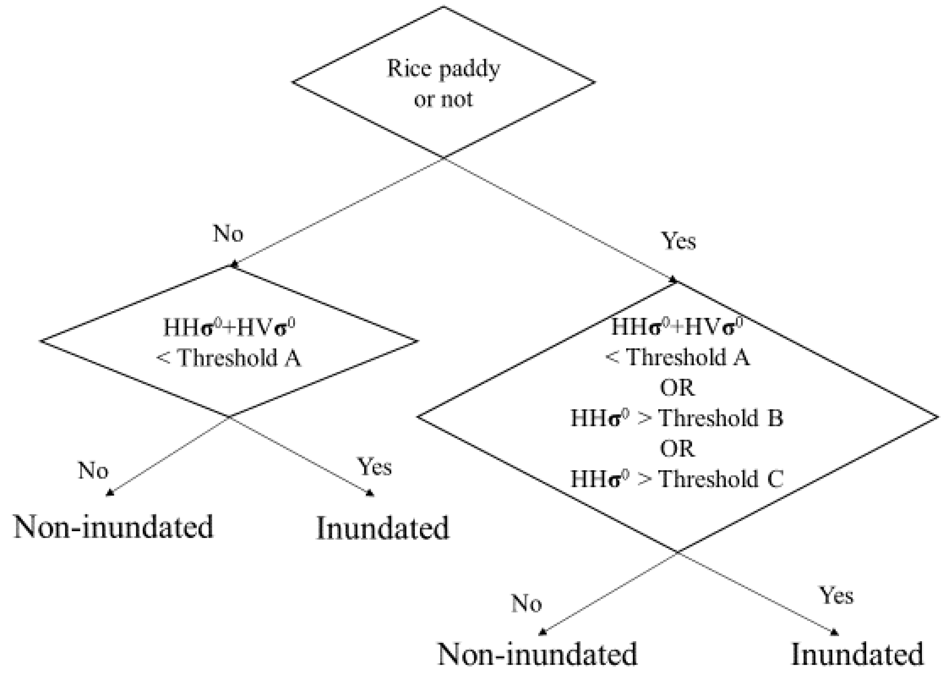
2.3. Inundation/Noninundation Classification Methods on Paddy Soils Covered by Rice Plants

From each ROI of each scene of the quadruple data, the values of 25–30 pixels were collected and averaged for the supervised classification with a hard-margin support vector machine (SVM) to distinguish inundated paddies and noninundated paddies. For ground-truth training data, we employed the abovementioned field observation data (i.e., field water levels and days after sowing/harvesting). The SVM-supervised classification was conducted with the statistical package R [35] and a kernlab library. Furthermore, the HH/HV σ⁰ values were collected and visualized using a 2D scatter plot method and then used as reference information to design the threshold line of inundated/noninundated soils with ScanSAR datasets.

The values of HH σ⁰ computed from the preprocessing of the ScanSAR datasets were analyzed to mask the rice paddies for further processing. First, we prepared datasets obtained from the same observation frames (i.e., the data coregistered with each other at the preprocessing step) with different observation dates. For the index of rice paddies observed in the frame, we calculated the differential of the sum of squared (DSS) values of each pixel using Equation (11) considering the rapid temporal dynamics of PALSAR’s HH σ⁰ in rice paddies (e.g., low HH σ⁰ values due to the specular reflection caused by flooded field water at the sowing stage and high HH σ⁰ values due to the double bounce from the flooded soil–rice plant state [24,49]):

$$DSS={{\displaystyle \sum }}_{i=1}^{n-1}{((HH{\sigma }_{i+1}^0- HH{\sigma }_i^0)\times 1000)}^2$$

(11)

where DSS is the differential of the sum of squared values of each pixel, n is the total number of all scenes obtained in the same observation frame on different observation dates, HH σ⁰ represents the HH σ⁰ values of PALSAR-2, and I is the time-series order of the PALSAR-2 scene in the frame (i.e., HH σ⁰_I+1 − HH σ⁰_I indicates the temporal difference of PALSAR-2’s HH σ⁰ values of each pixel between two adjacent observation times).

After the DSS of each pixel was calculated, the frequency distribution in each observation frame was computed. The frequency distribution was fast Fourier transformed and differentiated to compute its 2nd derivative value. For the threshold of rice paddies/non-rice paddies, we employed the value of DSS where the distribution is downward convex and its 2nd derivative value became 0. A sample of our masks of a PALSAR-2 observation frame, which is compared with a paddy mask reported in [22], is illustrated in Appendix B, Figure A1.

Using the rice paddy mask, we collected the local incidence angles, HH and HV σ⁰, of each rice paddy pixel from all of the scenes and then sorted them by every local incidence angle value. The three characteristics of inundated/noninundated rice paddies detected by the quadruple datasets are illustrated in Figure 2 as follows. (A) The values of HHσ⁰ + HVσ⁰ were smaller in inundated paddies than in noninundated paddies. (B) Even if the value of HHσ⁰ was at the same level between the inundated and noninundated paddies, the HVσ⁰ value was lower in inundated paddies than in noninundated paddies. (C) Even if the value of HVσ⁰ was at the same level between the inundated and noninundated paddies, the HHσ⁰ values were higher in inundated paddies than in noninundated paddies. Figure 2a) illustrates the three thresholds A–C (Equations (12)–(14)), as follows.

The values of HHσ⁰ + HVσ⁰ collected from all PALSAR-2 scene rice-paddy pixels (i.e., pixels detected as rice paddies by the mask computed by DSS (a sample of the masks is illustrated in Appendix B, Figure A1)) were sorted into every local incidence angle. The frequency distribution of the sorted values was fast Fourier transformed and then differentiated to compute the 2nd derivative value (e.g., Figure 3c). Threshold A is the value of HHσ⁰ + HVσ⁰ located between 2 peaks (low HHσ⁰ + HVσ⁰ values’ peak: inundated paddies; high HHσ⁰ + HVσ⁰ values’ peak: noninundated paddies) in the histogram of the HHσ⁰ + HVσ⁰ value (e.g., the histogram of pixels with a local incidence angle of 35 degrees, see Figure 3b). The 2nd derivative value shows the highest peak, e.g., the histogram of the 2nd derivative values with a local incidence angle of 35 degrees (see Figure 3c). The collected threshold A in every local incidence angle is plotted as Figure 3a. Considering the local incidence angle difference, threshold A was normalized via Equation (12) with the least squares method:

Threshold A (HHσ⁰+ HVσ⁰) = 243 × cosine(LIA)² − 361 × cosine(LIA) + 77.7

(12)

where Threshold A (HHσ⁰ + HVσ⁰) is the threshold A of inundated/noninundated paddies and LIA is the local incidence angle of each pixel of the PALSAR-2 data.

The values of HHσ⁰ collected from all PALSAR-2 scene rice-paddy pixels, i.e., pixels detected as rice paddies by the mask computed by DSS were sorted into every local incidence angle and every HVσ⁰-value (a sample of the masks is illustrated in Appendix B, Figure A1). The frequency distribution of the sorted values was fast Fourier transformed and then differentiated to compute the 2nd derivative value. The thresholds B and C are the values of HHσ⁰ located between two peaks (low HHσ⁰ value peak: noninundated paddies; high HHσ⁰ value peak: inundated paddies) that appeared in the histogram of the HHσ⁰ + HVσ⁰ value, where the 2nd derivative value shows the highest peak. Considering the 2D plot distribution of HHσ⁰ + HVσ⁰ values on every local incidence angle (e.g., Figure 3c), we built two thresholds of HHσ⁰ (i.e., thresholds B and C) with respect to the values of HV σ⁰ and the local incidence angle values following Equations (13) and (14) with the Hamiltonian–Monte Carlo method [34] implemented in RStan version 2.15.1 [35,36]. There were 9000 iterations, including 1000 warm-up periods, 10 thinnings, and four chains for both thresholds (B and C calculations). The difference in the data sorting group by the local incidence angle was considered as the random effect (e.g., group 1 as the pixels with the local incidence angle from 24.5 to 25.4 and group 2 as the pixels with the local incidence angle from 25.5 to 26.4, Figure 4).

$$\begin{array}{c}\mathrm{If}HV{\mathsf{\sigma }}^0>-31.5\mathrm{dB}\hfill \\ ThresholdB(HH{\sigma }^0)=0.550\times (HV{\mathsf{\sigma }}^0)+12.9\times \mathrm{cosine}(LIA)-11.2\end{array}$$

(13)

$$\begin{array}{c}\mathrm{If}HV{\mathsf{\sigma }}^0\le -31.5\mathrm{dB}\hfill \\ ThresholdC(HH{\sigma }^0)=1.036\times (HV{\mathsf{\sigma }}^0)-22.8\times \mathrm{sine}(LIA)+27.4\end{array}$$

(14)

where Threshold B, C (HHσ⁰) is threshold B, C of the inundated/noninundated paddies and LIA is the local incidence angle of each pixel of the PALSAR-2 data.

Using the SSD-derived rice paddy mask and thresholds A–C, the inundated/noninundated soils were classified as shown in Figure 5. The number of pixels classified as inundated soil was calculated as LSWC, and the LSWC maps (inundated soil pixel value = 1, noninundated soil pixel value = 0) were prepared. The LSWC maps from different observation frames were resampled at a 250 m resolution and coregistered. The validation of PALSAR-2-LSWC was conducted by a comparison with preprocessed AMSR-2-NDFI and MODIS-NDVI, NDWI and LSVC. The ratio between the cumulative ALOS-2/PALSAR-2 LSWC divided by the cumulative ALOS-2/PALSAR-2 observation times of all 105 scenes of PALSAR-2 ScanSAR data was mapped as a floodability map (Appendix C, Figure A2).

3. Results

3.1. Hierarchical Bayesian Models of CH₄ Emissions Based on Satellite-Sensed Phenology/Inundation Variables

The results of sampling with the Hamiltonian–Monte Carlo method to compute the parameters for hierarchical Bayesian models were successfully converged (Equations (1), (5)–(7): cumulative CH₄ emissions (g C m⁻² cropping⁻¹,

Table 1. Posterior distributions of parameters (α, β, γ, δ, ε, and ζ) in Equation (1) Ln(cum.Emi.) = α + β × inun.crop − γ×noninun.fallow − δ × inun.fallow + ε×straw − ζ × sulfate fitted by hierarchical Bayesian analysis, where “cum.Emi.” is the cumulative methane emission (g C m⁻² cropping⁻¹), “inun.crop” is the number of days of soil inundation (i.e., soil surface ≤ field-water level) during the cropping period (from sowing date to the harvest), “noninun.fallow”/“inun.fallow” are the days of soil noninundation/soil inundation during the fallow season just before the cropping period, “straw” is the value 0 or 1 (0 if the straw is removed or burned as described previously [8,9,10,11] after the carbon-emitting management is incorporated into the soil and 1 if all of the straw is directly incorporated into the soil without the carbon-emitting management), and “sulfate” is 0 or 1 (0 if the flux data are collected from alluvial soil and 1 if the flux data are collected from acid sulfate soils). All of the values are the mean ± standard deviation or the median.

	α	β	γ	δ	ε	ζ
Mean ± Standard deviation	2.91 ± 0.83	0.027 ± 0.012	0.083 ± 0.043	0.012 ± 0.008	0.43 ± 0.16	1.50 ± 1.14
Median	2.93	0.027	0.076	0.011	0.43	1.31

) and Equations (2)–(7): CH₄ fluxes (mg C m⁻² h⁻¹,

Table 2. Posterior distributions of parameters (η, θ, ι, κ, λ, μ, ν, ξ, ο, and π) in Equations (2)–(4) (Ln(flux) = Ln(η) + Ln(exp(−1 × θ × DAS) − exp(−1 × (θ + ι) × DAS) + κ) − Ln(1 + exp(−1 × λ × (DAS − μ×noninun.fallow))) + ν×inun.crop.10d + ξ × straw − ο × sulfate − π × inun.fallow) fitted by the hierarchical Bayesian analysis, where “flux” is the methane flux (mg C m⁻² h⁻¹), “DAS” is the number of days after sowing, “noninun.fallow” is the number of days of soil noninundation during the fallow season just before the cropping period, “inun.crop.10d” is the number of inundated days during the 10 days just before the target date (i.e., the sum of inundation days among x − 9 day, x − 8 day, …, x−1 day, x day; x as the target date), “straw” is 0 or 1 (0 if the straw is removed or burned, as described in multiple past papers [8,9,10,11], after the carbon-emitting management is incorporated into the soil and 1 if all of the straw is directly incorporated into the soil without the carbon-emitting management), and “sulfate” is 0 or 1 (0 if the flux data are collected from alluvial soil and 1 if the flux data are collected from acid sulfate soils). All of the values represent the mean ± standard deviation or the median.

	η	Θ	ι	κ	λ	μ	ν	ξ	ο	π
Mean ± Standard deviation	47.7 ± 36.0	0.099 ± 0.074	0.43 ± 0.26	0.019 ± 0.021	0.23 ± 0.22	1.03 ± 0.75	0.20 ± 0.10	0.28 ± 0.14	1.63 ± 1.57	0.00051 ± 0.00021
Median	42.0	0.073	0.45	0.011	0.16	0.88	0.188	0.27	1.39	0.00051

)). The Bayesian model of the cumulative CH₄ emissions in Equation (1), whose coefficients were substituted with their own posterior distribution mean values as described in Table 1, showed a positive linear relationship with the observed values (R² = 0.61, n = 588, Figure 6a). Regarding the daily flux, the Bayesian model of CH₄ fluxes in Equations (2)–(4), whose coefficients were substituted with their own posterior distribution mean values as described in Table 2, also showed a positive linear relationship with the observed values (R² = 0.34, n = 16,551, Figure 6b).

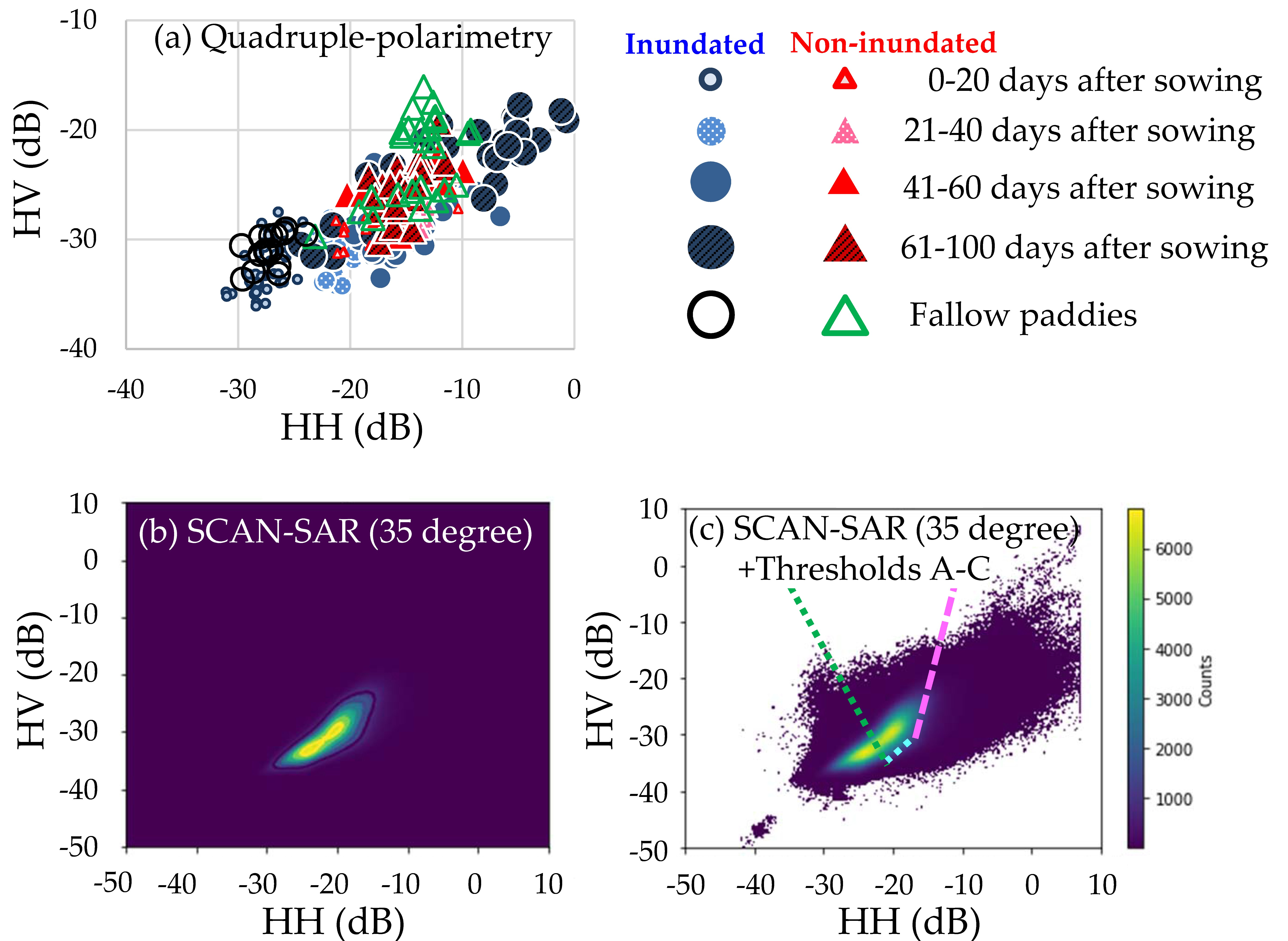
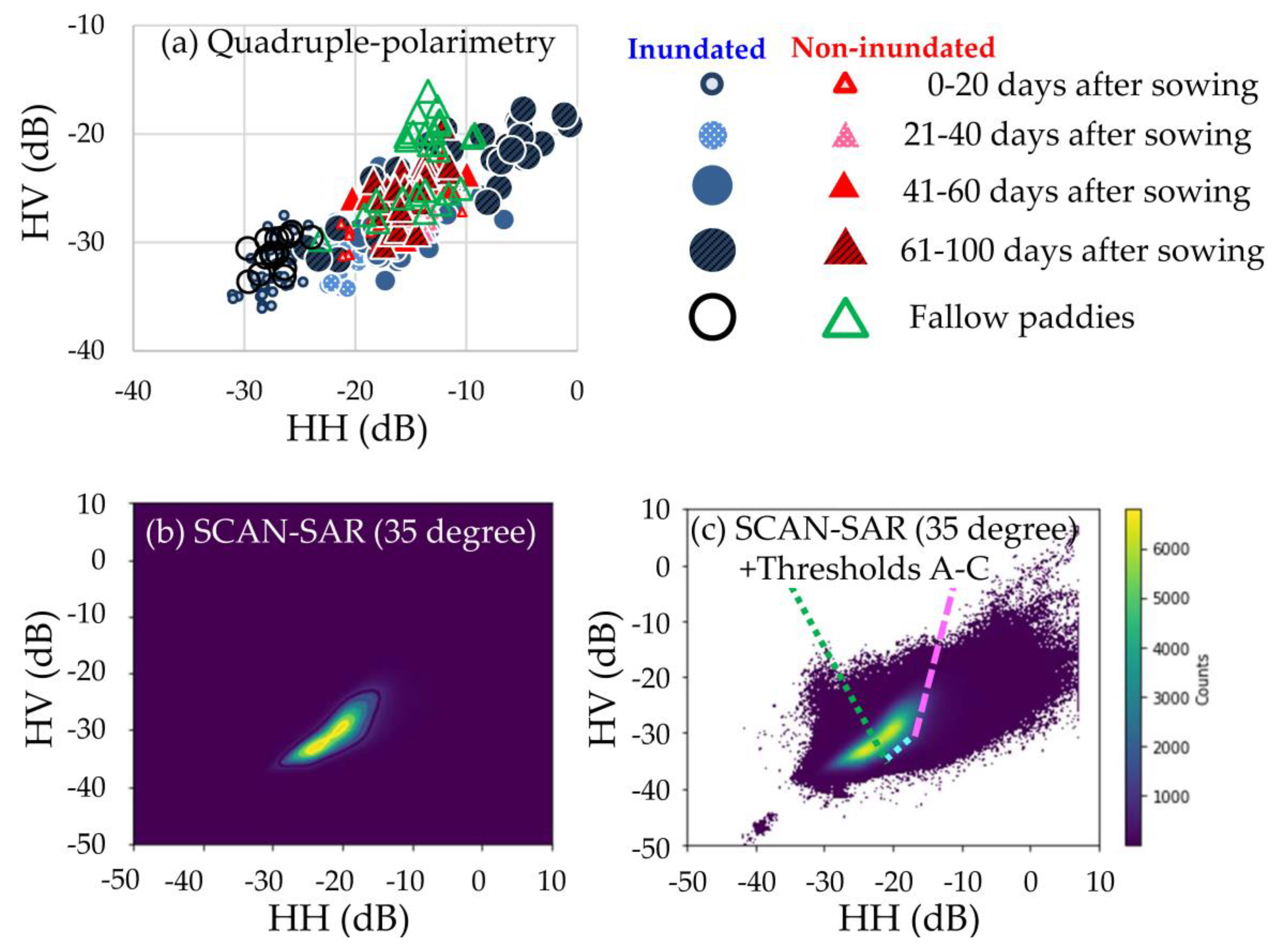
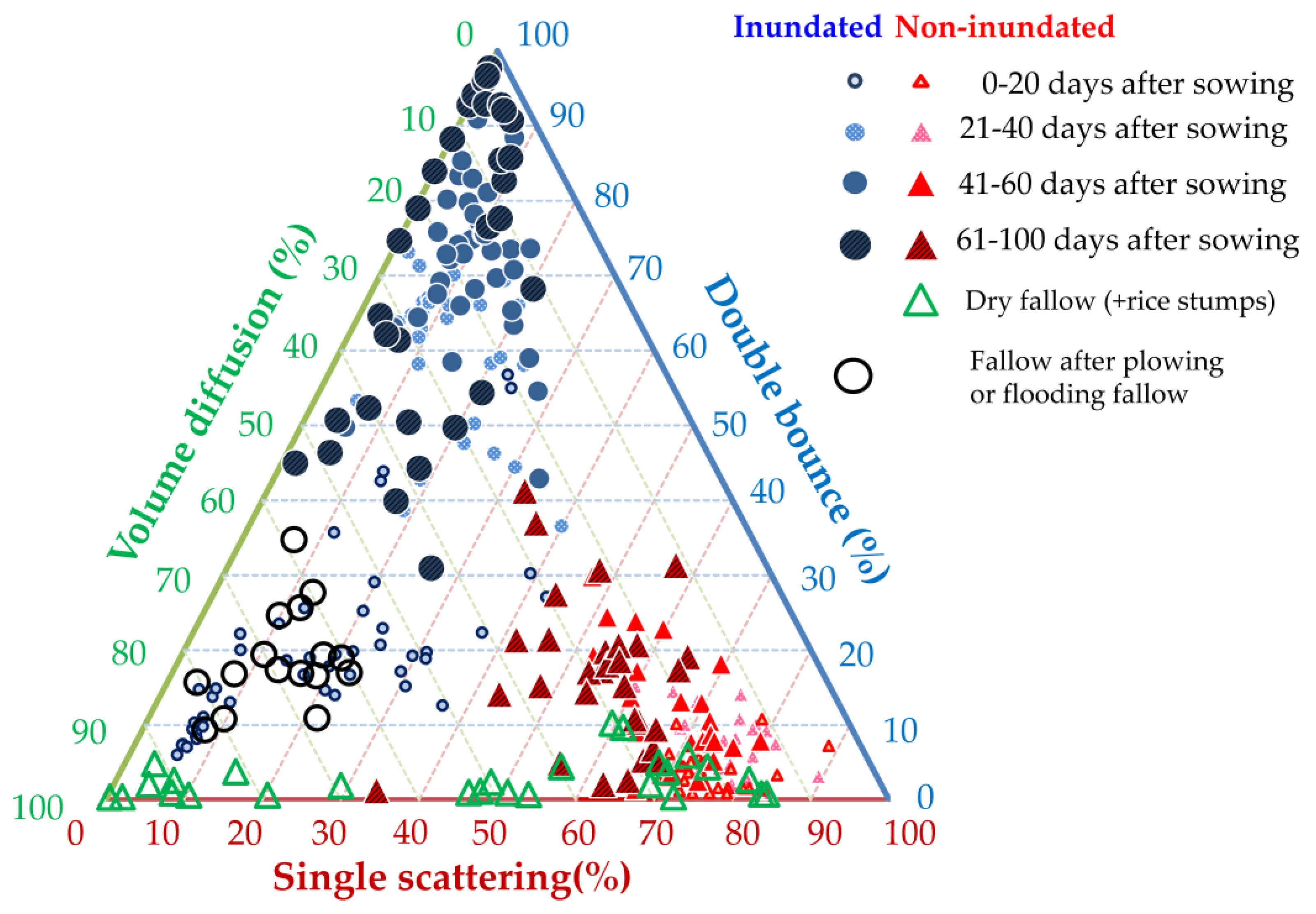
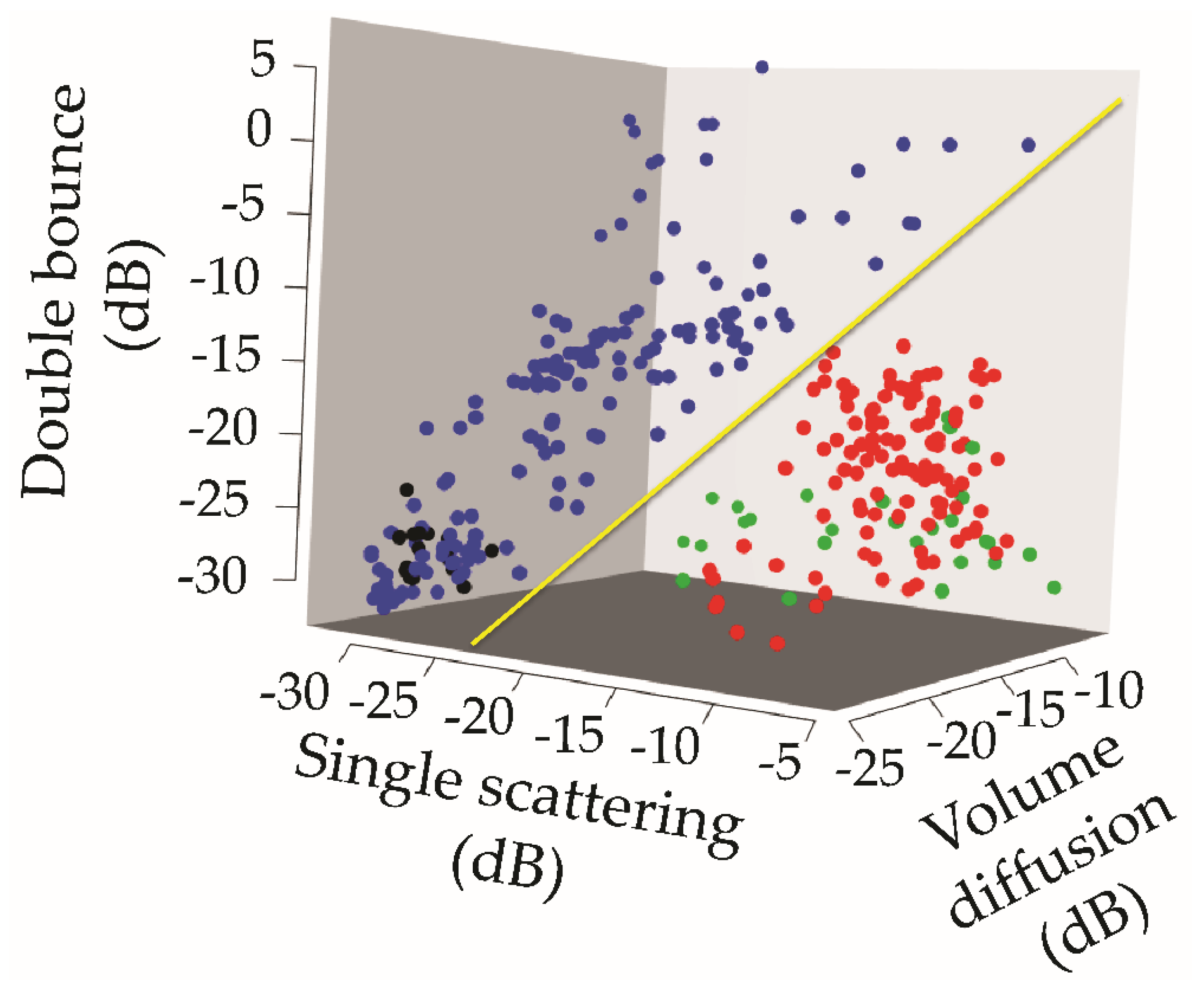
3.2. Characteristics of PALSAR-2 Quadruple Microwave Scattering in Inundated/Noninundated Rice Paddies

Inundated paddies whose soil surface is covered by field water were classified as either double-bounce dominant or volume-diffusion dominant groups (Figure 7). Single scattering and double bounce became negligible in the inundated flat-paddy soil, i.e., rice paddies up to 20 days after plowing or relatively small, inundated fallow paddies just after plowing. Even in the noninundated paddies, double-bounce dominance among the three scattering components tended to become more apparent in the days after sowing as the rice plant biomass increased. However, this trend was more apparent in the inundated paddies than in the noninundated paddies (Figure 7). Inundated paddies within 61–100 days after sowing showed a relatively wide distribution. On a dB basis, the inundated and noninundated paddies were classified without error, irrespective of their rice growth stage or the difference between their cropping and/or fallow seasons, by using the SVM-supervised classification (SVM-hyperplane: 0.281 × single scattering (dB) + 0.205 × volume diffusion (dB) − 0.233 × double bounce (dB) + 4.03, Figure 8).

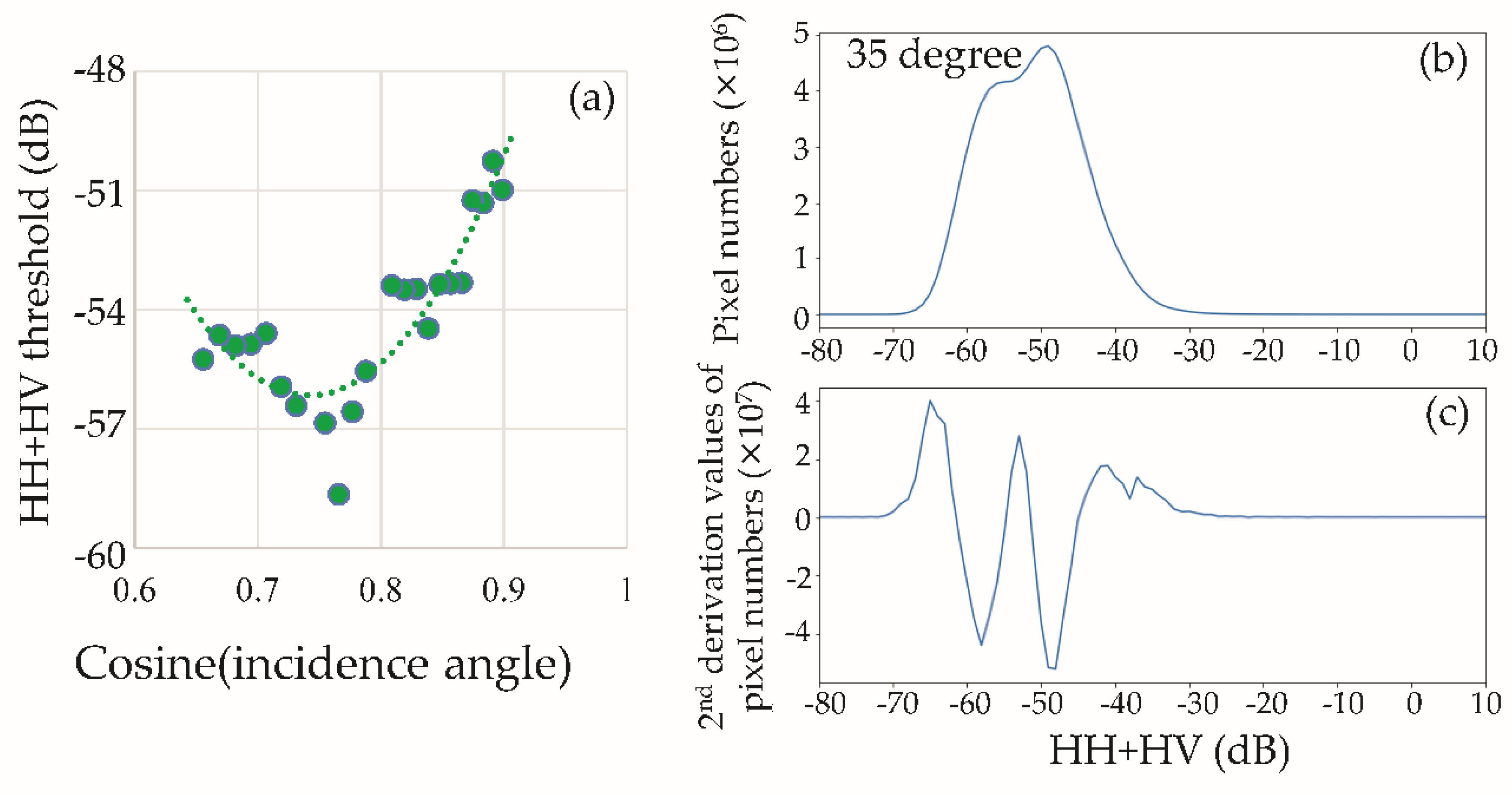
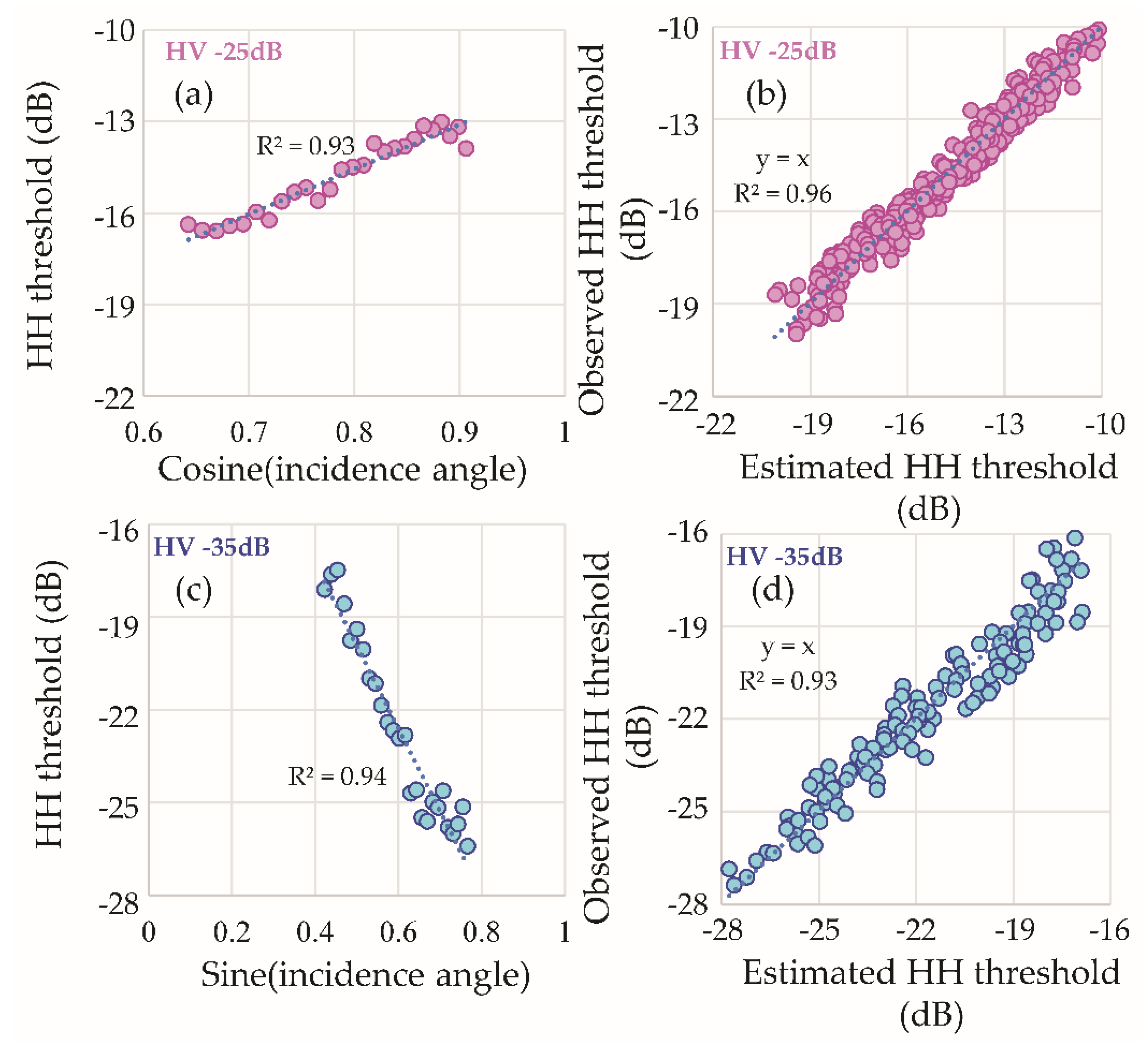
3.3. Inundation/Noninundation Classification with PALSAR-2-ScanSAR Data and Its Validation

The HHσ⁰ values of the rice paddies in the entire Mekong Delta tended to slightly increase in the dry season (approximately January to June) over the values in the rainy/flooding seasons (approximately July to December) (Figure 9). However, certain specific rice cropping paddies (e.g., areas enclosed with yellow open boxes in Figure 9) showed significantly higher HHσ⁰ values in the rainy/flooding season than in the dry season (Figure 10). Similar results were also obtained in the high spatial resolution (6 m) quadruple PALSAR-2 data (e.g., inundated rice paddies within 61 to 105 days after sowing in Figure 2a).

The AMSR-2 pixels, where the NDFI values were relatively high, tended to show only relatively high values of PALSAR-2 LSWC, and relatively low PALSAR-2 values became detectable as the AMSR-2-NDFI values decreased (Figure 11a). Similarly, the MODIS pixels, where the NDWI value is higher than 4%, tended to show low PALSAR-2-LSWC values less frequently as the NDWI value increased (Figure 11b). However, the high PALSAR-2-LSWC values were relatively frequently detected, and even the AMSR-2-NDFI values or MODIS-NDWI values were relatively low (Figure 11a,b). As the MODIS-LSVC/NDVI values increased, the PALSAR-2-LSWC values tended to be distributed widely (Figure 12c,d).

The PALSAR-2 floodability values (Appendix C, Figure A2) of the pixels tended to show a one-to-one relationship with the PALSAR-2-LSWC (Figure 12). However, certain pixels showed a slightly greater LSWC than the floodability values. In contrast, the pixels whose LSWC value is approximately 0 were densely detected in certain pixels, although the floodability values ranged from 0 to 60%.

4. Discussion

4.1. Hierarchical Bayesian Models of CH₄ Emissions Based on Satellite-Sensed Phenology/Inundation Variables

The successful convergence of the model parameters (Table 1 and Table 2) demonstrated the advantages of satellite-based rice phenology and soil-inundation/noninundation data in reproducing ground-observed CH₄ flux/emission data to a certain degree while maintaining high transparency of the entire methodology. Like the denitrification and decomposition (DNDC) biophysical process model [12], our model was designed considering the major microbial processes controlling the emission, i.e., Michaelis–Menten kinetics in which the CH₄ production rate is not regulated by the concentration when the fresh substrate concentration is high. However, the CH₄ production rate starts to become constrained by the remaining substrate days after sowing has passed and the amount of available substrate remaining becomes limited. Our model also considered the soil oxidation capacity by the electron acceptors. Then, the long-term and multipoint field observation data were parameterized with the Hamiltonian–Monte Carlo method. All of our model’s explanatory parameters were remote-sensed by satellites, the nonremote sensible parameters were omitted, e.g., fertilization rate/species/timing, statistical data, soil bio-physicochemical parameters, and rice physiological parameters, and the multipoint ground observation flux data were reproduced; therefore, the representative values of CH₄ fluxes/emissions could be computed with only the transparent satellite data, despite the high spatial heterogeneity of the fluxes and environmental factors, e.g., electron accepters and organic matter in the soil at the field-plot scale [17,18,50,51]. Furthermore, since our model requires only satellite data and soil GIS maps as the data input, a high spatial resolution map is applicable by inputting high spatial resolution satellite data. In addition, the emission status could be estimated in any target year if the satellite data are available. However, the parameters ζ and ο that were coefficients for the acid sulfate soil type had a large uncertainty and tended to underestimate the cumulative CH₄ emission from acid sulfate soil areas (Figure 6). The reason for this underestimation may have been the lack of observation site data to illustrate the variation in the spatial sulfate distribution, which inhibits methane production in soils by causing acetic acid and hydrogen to compete between methane formation and sulfate reduction [52,53]. Further observation of CH₄ emissions from more sites with different sulfate acidities is required to improve the parameters ζ and ο for a more accurate CH₄ emission from acid sulfate soil areas. Regarding the scalability of this methodology in another region, the indigenous CH₄ observation data should be used to reparameterize our model to confirm the reliability of the coefficient and to modify it for the target region.

Since unnecessarily increasing the number of parameters and explanatory variables risks altering the local optimization of each parameter, thus sacrificing their predictability and making it difficult to converge in statistical models, the models proposed in this study substituted certain scaling factors in the Tier1 IPCC guideline methodology [13] with only the transparent satellite-observable explanatory variables. To improve the accuracy of the models/methodology (i.e., higher determination coefficients, lower standard deviation of each parameter) while maintaining as much as possible the transparency of the entire methodology and its spatial resolution, the treatment of these heterogeneous and nonremote-sensed factors to reproduce the field observation data must be researched for the precise implementation of biophysical process models (e.g., the DNDC model [12]).

4.2. Characteristics of PALSAR-2 Quadruple Microwave Scattering in Inundated/Noninundated Rice Paddies

As described above, the satellite-based rice phenology and soil-inundation/noninundation data have the potential to reproduce the representative CH₄ flux/emission on a pixel basis with a high spatiotemporal resolution. However, few studies have addressed the inundation/noninundation classification of soils covered by vegetation without sacrificing the spatial resolution, unlike the satellite-based rice phenology study [19,20,21,22,23,24]. Although [54] reported lower C-band SAR (Environmental Satellite (ENVISAT)/Advanced SAR (ASAR), 5.6 cm wavelength) HH σ⁰ values in inundated paddies than those in noninundated paddies during the young stage (0–20 days after sowing), no such difference was detected during the later growing stages due to the saturation of the backscattering intensity in the rice plant canopy, which does not allow the microwave to penetrate the canopy and reach the soil surface. However, the present study demonstrated the ability to distinguish the inundated/noninundated paddy soils even when they were covered by large rice plants by employing the PALSAR-2 data. The results of the 6 m resolution quadruple data indicate that the intense double bounce occurs in inundated paddy soils that have a relatively large rice plant biomass, and the dominance of the double bounce tended to become greater with the number of days after sowing (Figure 7). The microwaves that bounced off the flat surface of the paddy water from the specular reflection would have also bounced off the rice plants’ biomass, which is called the “water–rice canopy interaction” [55], and similar results have been widely reported from SAR-based rice paddy monitoring studies (e.g., [12,23,24]). The reason inundated paddies within 61 to 100 days after sowing showed relatively wide distribution in Figure 7 may have been the difference in the rice lodging intensity. In contrast, the double bounce was relatively weak, with single scattering and volume diffusion becoming dominant in noninundated soils, particularly drained paddy soils in fallow seasons. These results indicate that rough soil surfaces cause dominant single-scattering characteristics in noninundated paddies. The apparent dominance of volume diffusion in the dry soil of the drained paddies during fallow seasons indicates that the microwaves penetrated soil or rice-stubble vegetation to cause a volume-diffusion-dominant backscatter (Figure 7).

4.3. Inundation/Noninundation Classification with PALSAR-2-ScanSAR Data

Referring to the characteristics of the 6-m-resolution PALSAR-2-HH&HV σ⁰ values, whose pixels had been classified as inundation/noninundation based on the 3-components’ decomposition results, we developed the inundation/noninundation rice paddy classification method (Figure 2). This method considers the bias derived from the difference in local incidence angles on the threshold (Figure 3 and Figure 4). To distinguish the inundated/noninundated areas, pixels with relatively low σ⁰ values are simply considered as inundated areas, while pixels with relatively high σ⁰ values are treated as noninundated areas regarding the specular reflection in inundated areas in related SAR studies [22,56]. The majority of the rice paddies monitored in this study also showed a similar tendency (i.e., slightly higher values of HH σ⁰ in the dry season than in the rainy/flooding seasons, Figure 9). However, significantly high HH σ⁰ values were detected in certain rice paddies, especially in the rainy/flooding seasons, in this study from ScanSAR data (Figure 9 and Figure 10). This result is consistent with the results of the 6-m-resolution data (i.e., the pixels of inundated rice paddies within 61 to 100 days after sowing with the high contribution double bounce (Figure 2 and Figure 7). These results indicated the need to treat the pixels with the HH σ⁰ values in a certain level as inundated rice paddies. As a similar scheme to our threshold calculation methodology, a past paper [57] also treated the pixels with HH σ⁰ values as “forest always flooded” to differentiate them from the pixels with lower HH σ⁰ values or “forest never flooded”. In this study, we also considered the difference of the local incidence angles of pixels in the threshold calculations. In most SAR studies, the backscattering coefficients of each microwaves (such as HH σ⁰) are normalized to correct the bias derived from local incidence angles with various methods (e.g., cosine correction methods [58,59] and semi-empirical correction methods [60,61]), and then thresholds are calculated based on the normalized backscattering coefficients. However, the values of HH σ⁰ consist of both single-scattering and double-bounce components, and each of the scattering components require a different normalization method or equation with different correction coefficients. Since the scattering components of the rice paddies widely varied, as illustrated in Figure 7, the intensity of the bias derived from the local incidence angle difference in the HH&HV σ⁰ values might also be different due to the difference in scattering components. Particularly for L-band SAR observation studies targeting the characterization of rice paddies, Bragg scattering-derived noise that occurred at specific local incidence angles needs to be considered [23,62,63]. Therefore, in this study, we normalized the threshold directly instead of the HH&HV σ⁰ values. To obtain representative thresholds that do not depend on the specificity of the image or observation frames, we employed 105 scenes of PALSAR-2 ScanSAR data with five different observation frames. Although clear linear relationships between threshold values and local incidence angles were observed for thresholds B and C (single scattering vs. double bounce), a nonlinear relationship was observed for threshold A (specular reflection vs. single scattering). As a result, the threshold A value reached its minimum at a local incidence angle of approximately 42 degrees. Consistent with this result, from their theoretical characterization results of Airborne SAR (Pi-SAR-L2) observations, the authors of a past paper [63] reported that backscattering reached a local minimum when the incidence angle was approximately 40 degrees in Japanese rice paddies due to Bragg scattering. Hence, our result might have appropriately classified inundated paddies and noninundated paddies by considering local incidence angle differences. Since the values of thresholds B and C clearly showed a linear relationship with the local incidence angles, in contrast to threshold A, the Bragg scattering might not have a significant effect on the difference between single scattering and double bounce compared with the difference between specular reflection and single scattering. Regarding the rice plant’s allocation in our targeted rice paddies, the rice plant density is significantly dense and heterogeneous due to the broadcasting direct sowing conventionally practiced in the area with a large sowing rate (196–223 kg ha⁻¹ [8,11]). To implement this methodology in the rice paddies of other countries, the model parameter may have to be recomputed empirically to consider the differences in the conventional rice planting practices (e.g., transplanting vs. direct sowing).

4.4. Comparison of PALSAR-2-ScanSAR LSWC with the Other Satellite Sensors

The validation results of AMSR-2-NDFI on PALSAR-2 LSWC showed a consistent inundation detection (i.e., few pixels with relatively low PALSAR-2-LSWC when the AMSR-2-NDFI or MODIS-NDWI values were relatively high). These results indicated the advantage of the PALSAR-2-LSWC that detects inundated pixels consistently with AMSR-2-NDFI and MODIS-NDWI if the inundated soil is not covered by rice plants. However, an inconsistency was also found, in which pixels with relatively high PALSAR-2-LSWC were frequently detected even when the values of AMSR-2-NDFI or MODIS-NDWI were low. These results indicated that the PALSAR-2-LSWC may be able to detect inundated soils covered by rice plants, although the AMSR-2-NDFI of MODIS-NDWI could not detect them due to the rice plant canopy disturbance. Notably, as the MODIS-NDVI/LSVC values increased, the PALSAR-2-LSWC values tended toward a wide distribution, and a dense pixel distribution was allocated where the MODIS-LSVC was approximately 100% or the NDVI values were approximately 6–9%. These results indicated that a large part of the inundated soil is covered by rice plants and that a method to classify inundated soils and noninundated soils that cannot be classified by AMSR-2 or MODIS is essential for the regional CH₄ emissions. As further validation, the employment of the GNSS-R technique [28] or the other new L-Band SARs (e.g., ALOS-4 and NASA-ISRO-SAR) is desirable for improving the methodology with a higher spatiotemporal resolution. Although the one-to-one relationship between the PALSAR-2-LSWC and the floodability indicated a consistent water body (e.g., Mekong River, subcanals, and ponds), inconsistencies between the PALSAR-2-LSWC and floodability were also found, particularly in pixels with approximately 0–50% floodability. Higher values of the LSWC than the floodability indicate inundation due to rainfall or irrigation in rice paddies, and lower values may indicate the drainage of rice paddies or drought. Since the pixels with approximately 0% PALSAR-2-LSWC were frequently found irrespective of floodability, it was considered that the drainage practice or drought may control the LSWC more rapidly than irrigation or rainfall. Regarding the floodability map (Appendix C, Figure A2), relatively high floodability values were detected in acid sulfate soil regions [64] of the Mekong Delta located in the northeast region (Dong Thap Province and Long An Province), the western-middle region (border between southeastern Kieng Giang Province and Western Can Tho City), and the south-middle region (northern area of Bac Rieu Province and the south area of Hau Giang Province) but not the western-north region of the delta (northern area of the Kieng Giang Province and western area of the An Giang Province). Notably, alluvial soil regions located in An Giang and Can Tho City, where a study of the water-saving intermittent irrigation practice called alternate wetting and drying (AWD) has been underway [8,9,30,31,24], tended to show relatively low values of floodability, even though triple rice cropping is widely practiced in the area. Although further validation is required, it appears that the spatial distribution of floodability can indicate the differences in the regional AWD dissemination status over recent years, the infrastructure of the irrigation or dyke system, and the regional CH₄ emission intensities. A similar study on AWD dissemination [65] assessed the suitability of the AWD based on satellite climate data and field data of the water percolation rate. Although this type of index, such as the Keeth–Byram Drought Index (KBDI), which is used for groundwater estimation in tropical peatland and soil organic matter decomposition (i.e., CO₂ emissions from soil) [66], can also be considered as another validation tool in this study, the water level in the subcanals diurnally fluctuates drastically and is regionally different due to the tidal movement in the whole delta, which would intensely affect the field/groundwater levels [8,9,10,11]. In addition, artificial impacts, such as the application of pumping irrigation in each rice paddy, and drainage or irrigation gate operation on each dyke system, would also lead to heterogeneous inundation. Considering these factors affecting the heterogeneity of the field inundation status, our methodology, with a high spatial resolution, has the advantage of precisely monitoring a heterogeneous field inundation status.

5. Conclusions

This study demonstrated the potential for a satellite data-based transparent methodology to reproduce field-observed CH₄ emissions by substituting certain major scaling factors of the IPCC-Tier 1 methodology and the potential for PALSAR-2 data to be used to monitor the field inundation status with a high spatial resolution, even when the paddy fields are covered by clouds or rice plants. We also proposed an inundated/noninundated paddy classification methodology considering the intense double bounce that occurs in inundated paddies with a high rice plant biomass, which considers the effects of bias derived from local differences in incidence angle on the backscattering coefficients due to the differences in scattering components.

References

1. Ciais, P.; Sabine, C.; Bala, G.; Bopp, L.; Brovkin, V.; Canadell, J.; Chhabra, A.; DeFries, R.; Galloway, J.; Heimann, M.; et al. The Physical Science Basis. Contribution of Working Group I to the Fifth Assessment Report of the Intergovernmental Panel on Climate Change; Stocker, T.F., Qin, D., Plattner, G.K., Tignor, M.M.B., Allen, S.K., Boschung, J.B., Nauels, A., Xia, Y., Bex, V., Midgley, P.M., Eds.; Cambridge University Press: Cambridge, UK; New York, NY, USA, 2013. [Google Scholar]
2. Schaefer, H.; Fletcher, S.E.M.; Veidt, C.; Lassey, K.R.; Brailsford, G.W.; Bromley, T.M.; Dlugokencky, E.J.; Michel, S.E.; Miller, J.B.; Levin, I.; et al. A 21st-century shift from fossil-fuel to biogenic methane emissions indicated by 13 CH4. Science 2016, 352, 80–84. [Google Scholar] [CrossRef] [PubMed]
3. Smith, P.; Martino, D.; Cai, Z.C.; Gwary, D.H.J. Greenhouse gas mitigation in agriculture. Philos. Trans. R. Soc. B Biol. Sci. 2008, 363, 789–813. [Google Scholar] [CrossRef] [PubMed] [Green Version]
4. Alexandratos, N.; Bruinsma, J. World Agriculture towards 2030/2050: The 2012 Revision; ESA Working paper; FAO: Rome, Italy, 2012; Volume 12. [Google Scholar]
5. FAOSTAT. FAO Statistical Databases. Available online: http://faostat.fao.org/ (accessed on 23 January 2017).
6. General Statistics Office of Viet Nam. Statistical Yearbook of Vietnam 2014; Statistical Publishing House: Hanoi, Vietnam, 2014. [Google Scholar]
7. Son, N.T.; Chen, C.F.; Chen, C.R.; Duc, H.N.; Chang, L.Y. A phenology-based classification of time-series MODIS data for rice crop monitoring in Mekong Delta, Vietnam. Remote Sens. 2013, 6, 135–156. [Google Scholar] [CrossRef]
8. Arai, H. The Anthropogenic Greenhouse Gas Emission from Tropical High Carbon Reservoirs. Chiba University Library Online Public Library Catalog. 2015. Available online: http://opac.ll.chiba-u.jp/da/curator/900119174/HMA_0068.pdf (accessed on 11 April 2018). (In Japanese).
9. Arai, H.; Takeuchi, W.; Oyoshi, K.; Nguyen, L.D.; Tachiba, T.; Inubushi, K. Regional evaluation on greenhouse gas-mitigation & yield-increase performance of a water-saving irrigation practice’s dissemination in rice paddies in the Mekong Delta. Monit. Glob. Environ. Disaster Risk Assess. Space IIS Forum Proc. 2018, 26, 43–50. [Google Scholar]
10. Van, N.P.H.; Nga, T.T.; Arai, H.; Hosen, Y.; Chiem, N.H.; Inubushi, K. Rice straw management by farmers in a triple rice production system in the Mekong Delta, Viet Nam. Trop. Agric. Dev. 2014, 58, 155–162. [Google Scholar]
11. Arai, H.; Hosen, Y.; Pham Hong, V.N.; Chiem, N.H.; Inubushi, K. Greenhouse gas emissions derived from rice straw burning and straw-mushroom cultivation in a triple rice cropping system in the Mekong Delta. Soil Sci. Plant Nutr. 2015, 61, 719–735. [Google Scholar] [CrossRef]
12. Torbick, N.; Salas, W.; Chowdhury, D.; Ingraham, P.; Trinh, M. Mapping rice greenhouse gas emissions in the Red River Delta, Vietnam. Carbon Manag. 2017, 8, 99–108. [Google Scholar] [CrossRef]
13. Lasco, R.D.; Ogle, S.; Raison, J.; Verchot, L.; Wassmann, R.; Yagi, K.; Bhattacharya, S.; Brenner, J.S.; Daka, J.P.; González, S.P.; et al. (Eds.) IPCC Guidelines for National Greenhouse Gas Inventories Volume 4: Agriculture, Forestry and Other Land Use; The Institute for Global Environmental Strategies: Hayama, Japan, 2006; pp. 5.1–5.66. [Google Scholar]
14. Basak, R. Monitoring, Reporting, and Verification Requirements and Implementation Costs for Climate Change Mitigation Activities: Focus on Bangladesh, India, Mexico, And Vietnam; Working Paper; CGIAR Research Program on Climate Change Agriculture and Food Security (CCAFS): Wageningen, The Netherlands, 2016; Volume 162, p. 28. [Google Scholar]
15. Yan, X.; Akiyama, H.; Yagi, K.; Akimoto, H. Global estimations of the inventory and mitigation potential of methane emissions from rice cultivation conducted using the 2006 Intergovernmental Panel on Climate Change Guidelines. Glob. Biogeochem. Cycles 2009, 23, 1–15. [Google Scholar] [CrossRef]
16. United Nations Framework Convention on Climate Change. Clean Development Mechanism ASB0008 Standardized Baseline: Methane Emissions from Rice Cultivation in the Republic of the Philippines. 2015. Available online: https://cdm.unfccc.int/filestorage/e/x/t/extfile-20150728141509407-ASB0008.pdf/ASB0008.pdf?t=Tld8cDcwd2lzfDDr3USmzWHg7TTXN0qQhGm_ (accessed on 11 April 2018).
17. Nishina, K.; Akiyama, H.; Nishimura, S.; Sudo, S.; Yagi, K. Evaluation of uncertainties in N2O and NO fluxes from agricultural soil using a hierarchical Bayesian model. J. Geophys. Res. Biogeosci. 2012, 117, G4. [Google Scholar] [CrossRef]
18. Nihina, K. State of the art: Evaluation of carbon, nitrogen and water cycling in natural and agro ecosystems in field to global scale. 4. Application of spatial statistics in soil science. J. Soil Sci. Plant Nutr. 2017, 88, 339–345. (In Japanese) [Google Scholar]
19. Oyoshi, H.; Sobue, S.; Takeuchi, W. Development of complicated rice crop calendar in Southeast Asia with time-series MODIS data. In Proceedings of the 2013 Second International Conference on Agro-Geoinformatics (Agro-Geoinformatics), Fairfax, VA, USA, 12–16 August 2013; pp. 444–447. [Google Scholar]
20. Jonai, H.; Takeuchi, W. Comparison between global rice paddy field mapping and methane flux data from GOSAT. In Proceedings of the Geoscience and Remote Sensing Symposium (IGARSS) IEEE International, Quebec City, QC, Canada, 13–18 July 2014; pp. 2098–2101. [Google Scholar]
21. Phan, T.H.; Le Toan, T.; Bouvet, A.; Nguyen, L.D.; Pham Duy, T.; Zribi, M. Mapping of Rice Varieties and Sowing Date Using X-Band SAR Data. Sensors 2018, 18, 316–339. [Google Scholar] [CrossRef] [PubMed]
22. Le Toan, T.; Phan, T.H.; Bouvet, A. Rice Monitoring Using Sentinel-1 Data. International Meeting on Land Use and Emissions in South/Southeast Asia 2016. Available online: http://sari.umd.edu/sites/default/files/Thuy_LeToan.pdf (accessed on 11 April 2018).
23. Rosenqvist, A. Temporal and spatial characteristics of irrigated rice in JERS-1 L-band SAR data. Int. J. Remote Sens. 1999, 20, 1567–1587. [Google Scholar] [CrossRef]
24. Wang, C.; Wu, J.; Zhang, Y.; Pan, G.; Qi, J.; Salas, W.A. Characterizing L-band scattering of paddy rice in southeast China with radiative transfer model and multitemporal ALOS/PALSAR imagery. IEEE Trans. Geosci. Electron. 2009, 47, 988–998. [Google Scholar] [CrossRef]
25. Xiao, X.; Boles, S.; Frolking, S.; Li, C.; Babu, J.Y.; Salas, W.; Moore, B. Mapping paddy rice agriculture in South and Southeast Asia using multi-temporal MODIS images. Remote Sens. Environ. 2006, 100, 95–113. [Google Scholar] [CrossRef]
26. Li, X.; Takeuchi, W. Land Surface Water Coverage Estimation with PALSAR and AMSR-E for Large Scale Flooding Detection. Terr. Atmos. Ocean. Sci. 2016, 27, 473–480. [Google Scholar] [CrossRef]
27. Melack, J.M.; Hess, L.L.; Gastil, M.; Forsberg, B.R.; Hamilton, S.K.; Lima, I.B.; Novo, E.M. Regionalization of methane emissions in the Amazon Basin with microwave remote sensing. Glob. Chang. Biol. 2004, 10, 530–544. [Google Scholar] [CrossRef]
28. Nghiem, S.V.; Zuffada, C.; Shah, R.; Chew, C.; Lowe, S.T.; Mannucci, A.J.; Cardellach, E.; Brakenridge, G.R.; Geller, G.; Rosenqvist, A. Wetland monitoring with Global Navigation Satellite System reflectometry. Earth Space Sci. 2017, 4, 16–39. [Google Scholar] [CrossRef] [PubMed] [Green Version]
29. Shimada, M. Japan Aerospace Exploration Agency-Earth Observation Research Center. ALOS-2 characteristics, CAL/VAL results and operational status. ALOS Kyoto & Carbon Initiative 21th Science Team Meeting 2014. Available online: http://www.eorc.jaxa.jp/ALOS/kyoto/dec2014_kc21/pdf/3-02_KC21_ALOS-2_Shimada-JAXA.pdf (accessed on 11 April 2018). (In Japanese).
30. Taminato, T.; Matsubara, E. Impacts of two types of water-saving irrigation system on greenhouse gas emission reduction and rice yield in paddy fields in the Mekong delta. IDRE Journal 2016, No. 303. 84, I_195-I_200. Available online: https://www.jstage.jst.go.jp/article/jsidre/84/3/84_I_195/_pdf (accessed on 11 April 2018). (In Japanese).
31. Ishido, K.; Nguyen, X.L.; Taminato, T.; Hosen, Y.; Arai, H. Dissemination of a Water-Saving Technology to Paddy Fields in the Mekong Delta. Annual Meeting of the Japanese Society of Irrigation, Drainage and Rural Engineering. 2016. Available online: http://soil.en.a.u-tokyo.ac.jp/jsidre/search/PDFs/16cd/manuscript_pdf/[6-28].pdf (accessed on 11 April 2018). (In Japanese).
32. Whittaker, E.T.; Robinson, G. Trapezoidal and Parabolic rules. In The Calculus Observation: A Treatise of Numerical Mathematics; Read Books: Dover, NY, 1967; Chapter VII 77; pp. 156–158. [Google Scholar]
33. Inubushi, K.; Saito, H.; Arai, H.; Ito, K.; Endoh, K.; Yashima, M.M. Effect of oxidizing and reducing agents in soil on methane production in Southeast Asian paddies. Soil Sci. Plant Nutr. 2018, 64, 84–89. [Google Scholar] [CrossRef]
34. Hoffman, M.D.; Gelman, A. The No-U-Turn sampler: Adaptively setting path lengths in Hamiltonian Monte Carlo. J. Mach. Learn. Res. 2014, 15, 1549–1591. [Google Scholar]
35. R Development Core team and others R: A language and environment for statistical computing. R Found. Stat. Comput. 2005. Available online: http://www.r-project.org (accessed on 19 April 2017).
36. Stan Development Team RStan: The R interface to Stan, Version 2.15. Available online: http://mc-stan.org/rstan.html (accessed on 19 April 2017).
37. Japan Aerospace Exploration Agency-Earth Observation Research Center/ALOS-2 Project Team. Update of the Radiometric and Polarimetric Calibration for the PALSAR-2 Standard Product. Available online: http://www.eorc.jaxa.jp/ALOS-2/en/calval/PALSAR2_CalVal_Result_JAXA_20170323_En.pdf (accessed on 11 April 2018).
38. Freeman, A.; Durden, S.L. A three-component scattering model for polarimetric SAR data. IEEE Geosci. Remote Sens. 1998, 36, 963–973. [Google Scholar] [CrossRef]
39. Pottier, E.; Ferro-Famil, L.; Allain, S.; Cloude, S.; Hajnsek, I.; Papathanassiou, K.; Moreia, A.; Williams, M.; Minchella, A.; Lavalle, M.; et al. Overview of the PolSARpro V4.0 software. The open source toolbox for polarimetric and interferometric polarimetric SAR data processing. In Proceedings of the 2009 IEEE International Geoscience and Remote Sensing Symposium, Cape Town, South Africa, 12–17 July 2009; Volume 4, p. IV-936. [Google Scholar]
40. Japan Aerospace Exploration Agency-Earth Observation Research Center/ALOS-2 Project Team. Calibration Factors (CF, A) Determined by JAXA CalVal Observations (ver. Mar. 23, 2017). Available online: http://www.eorc.jaxa.jp/ALOS-2/calval/CalibrationFactors_PALSAR2_v20170323.pdf (accessed on 11 April 2018).
41. Lopes, A.; Touzi, R.; Nezry, E. Adaptive speckle filters and scene heterogeneity. IEEE Geosci. Remote Sens. 1990, 28, 992–1000. [Google Scholar] [CrossRef]
42. De Grandi, G.F.; Leysen, M.; Lee, J.S.; Schuler, D. Radar Reflectivity Estimation Using Multiple SARScenes of the Same Target: Technique and Applications. Available online: http://ieeexplore.ieee.org/xpl/login.jsp?tp=&arnumber=615338&url=http%3A%2F%2Fieeexplore.ieee.org%2Fiel3%2F4810%2F13419%2F00615338.pdf%3Farnumber%3D615338 (accessed on 5 June 2017).
43. Meier, E.; Frei, U.; Nüesch, D. Precise Terrain Corrected Geocoded Images. Available online: http://citeseer.uark.edu:8080/citeseerx/showciting;jsessionid=A5ABC292190B6C7331543DA9D7EDE934?cid=192163 (accessed on 5 June 2017).
44. Holecz, F.; Meier, E.; Piesbergen, J.; Nüesch, D. Topographic effects on radar cross section. In Proceedings of the CEOS SAR Calibration Workshop, Noordwijk, The Netherlands, 20–24 September 1993; pp. 20–24. [Google Scholar]
45. Asilo, S.; de Bie, K.; Skidmore, A.; Nelson, A.; Barbieri, M.; Maunahan, A. Complementarity of two rice mapping approaches: Characterizing strata mapped by hypertemporal MODIS and rice paddy identification using multitemporal SAR. Remote Sens. 2014, 6, 12789–12814. [Google Scholar] [CrossRef]
46. Sawada, Y.; Mitsuzuka, N. Development of a time-series model filter for high revisit satellite data. In Proceedings of the 2nd International VEGETATION Users Conference; European Union: Brussels, Belgium, 2005; Available online: http://www.rsgis.ait.ac.th/~honda/textbooks/advrs/LMF_p83Sawada_SPOT.pdf (accessed on 11 April 2018).
47. Sawada, H.; Sawada, Y.; Matsuura, Y. Observation of forest environment changes in Siberia. International Archives of the Photogrammetry. Remote Sens. Spat. Inf. Sci. 2018, 38, 8. [Google Scholar]
48. Sezgin, M.; Sankur, B. Survey over image thresholding techniques and quantitative performance evaluation. J. Electron. Imaging 2006, 13, 146–168. [Google Scholar]
49. Zhang, Y.; Wang, C.; Wu, J.; Qi, J.; Salas, W.A. Mapping paddy rice with multitemporal ALOS/PALSAR imagery in southeast China. Int. J. Remote Sens. 2009, 30, 6301–6315. [Google Scholar] [CrossRef]
50. Yanai, J.; Lee, C.K.; Kaho, T.; Iida, M.; Matsui, T.; Umeda, M.; Kosaki, T. Geostatistical analysis of soil chemical properties and rice yield in a paddy field and application to the analysis of yield-determining factors. Soil Sci. Plant Nutr. 2001, 47, 291–301. [Google Scholar] [CrossRef] [Green Version]
51. Liu, X.M.; Xu, J.M.; Zhang, M.K.; Huang, J.H.; Shi, J.C.; Yu, X.F. Application of geostatistics and GIS technique to characterize spatial variabilities of bioavailable micronutrients in paddy soils. Environ. Geol. 2004, 46, 189–194. [Google Scholar] [CrossRef]
52. Hori, K.; Inubushi, K.; Matsumoto, S.; Wada, H. Competition of acetic acid between methane formation and sulfate reduction in paddy soil. J. Soil Sci. Plant Nutr. 1990, 61, 572–578. [Google Scholar]
53. Hori, K.; Inubushi, K.; Matsumoto, S.; Wada, H. Competition for hydrogen between methane formation and sulfate reduction in a paddy soil. J. Soil Sci. Plant Nutr. 1993, 64, 363–367. [Google Scholar]
54. Lam Dao, N.; Le Toan, T.; Apan, A.A.; Bouvet, A.; Young, F.; Le Van, T. Effects of changing rice cultural practices on C-band synthetic aperture radar backscatter using Envisat advanced synthetic aperture radar data in the Mekong River Delta. J. Appl. Remote Sens. 2009, 3, 033563. [Google Scholar] [Green Version]
55. Le Toan, T.; Ribbes, F.; Wang, L.F.; Floury, N.; Ding, K.H.; Kong, J.A.; Fujita, M.; Kurosu, T. Rice crop mapping and monitoring using ERS-1 data based on experiment and modeling results. IEEE Trans. Geosci. Remote Sens. 1997, 35, 41–56. [Google Scholar] [CrossRef]
56. Matgen, P.; Hostache, R.; Schumann, G.; Pfister, L.; Hoffmann, L.; Savenije, H.H.G. Towards an automated SAR-based flood monitoring system: Lessons learned from two case studies. Phys. Chem. Earth 2011, 36, 241–252. [Google Scholar] [CrossRef]
57. Martinez, J.M.; Le Toan, T. Mapping of flood dynamics and spatial distribution of vegetation in the Amazon floodplain using multitemporal SAR data. Remote Sens. Environl. 2007, 108, 209–223. [Google Scholar] [CrossRef]
58. Ulaby, F.T.; Dobson, M.C. Handbook of Radar Scattering Statistics for Terrain (Artech House Remote Sensing Library); Artech House: Norwood, MA, USA, 1989. [Google Scholar]
59. Mladenova, I.E.; Jackson, T.J.; Bindlish, R.; Hensley, S. Incidence angle normalization of radar backscatter data. IEEE Trans. Geosci. Remote Sens. 2013, 51, 1791–1804. [Google Scholar] [CrossRef]
60. Topouzelis, K.; Singha, S.; Kitsiou, D. Incidence angle normalization of Wide Swath SAR data for oceanographic applications. Open Geosci. 2016, 8, 450–464. [Google Scholar] [CrossRef]
61. Zhao, L.; Chen, E.; Li, Z.; Zhang, W.; Gu, X. Three-step semi-empirical radiometric terrain correction approach for PolSAR data applied to forested areas. Remote Sens. 2017, 9, 269–299. [Google Scholar] [CrossRef]
62. Xuan, V.T.; Matsui, S. Development of farming systems in the Mekong Delta of Vietnam; HCMC Publishing House: Ho Chi Minh City, Vietnam, 1998; p. 25. [Google Scholar]
63. Ishitsuka, N. The Scatter Characteristic of Rice Paddy Fields Using L Band Multi Polarimetric Satellite SAR Observation. In CD Proceedings of the First Joint PI Symposium of ALOS Data Nodes for ALOS Science Program in Kyoto; JAXA: Chofu, Japan, 19–23 November 2007.
64. Arii, M.; Yamada, H. Rice paddy monitoring by L-band MIMP SAR approach. In Proceedings of the 2017 IEEE International Geoscience and Remote Sensing Symposium (IGARSS), Fort Worth, TX, USA, 23–28 July 2017; pp. 2442–2445. [Google Scholar]
65. Nelson, A.; Wassmann, R.; Sander, B.O.; Palao, L.K. Climate-determined suitability of the water saving technology” Alternate wetting and drying” in rice systems: A scalable methodology demonstrated for a province in the Philippines. PLoS ONE 2015, 10, e0145268. [Google Scholar] [CrossRef] [PubMed]
66. Takeuchi, W.; Hirano, T.; Roswintiarti, O. Estimation Model of Ground Water Table at Peatland in Central Kalimantan, Indonesia. In Tropical Peatland Ecosystems; Springer: Tokyo, Japan, 2016; pp. 445–453. [Google Scholar]
Figure 1. Flowchart of the study outlining the data, processing, and analysis. PALSAR-2, AMSR-2, MODIS, and HH HV σ0 refer to the Phased Array type L-band Synthetic Aperture Radar, Advanced Microwave Scanning Radiometer-2, MODerate resolution Imaging Spectroradiometer, and the backscattering coefficient of HH/HV microwaves, respectively.
Remotesensing 10 01438 g001
Figure 2. Scatter plot of ALOS-2/PALSAR-2-quadruple polarimetric high spatial resolution (3 m) data of the backscattering coefficients of HH and HV microwave (n = 313, (a)), a sample of the 2D histogram of ScanSAR data illustrated with contours (b), and the noncontour histogram with three thresholds A–C (c). The horizontal axes in the subfigures (ac) indicate HHσ0 values, and the vertical axes indicate HVσ0 values. The lightest/smallest closed blue circles (n = 48) in subfigure (a) indicate the mean value among 25–30 pixels of an inundated paddy ROI (up to 20 days after sowing). The second lightest/smallest dotted blue circles (n = 30) represent 21–40 days after sowing. The third lightest/smallest closed blue circles (n = 40) represent 41–60 days after sowing. The darkest hatched blue circles (n = 32) represent 61–100 days after sowing. The black open circles (n = 16) represent the fallow period, just after plowing, or inundated fallow. The smallest red open triangles (n = 36) in the subfigure (a) indicate the mean value among 25–30 pixels of a noninundated paddy ROI (0–20 days after sowing). The second lightest/smallest dotted red triangles (n = 28) represent 21–40 days after sowing; the third lightest/smallest closed red triangles (n = 26) represent 41–60 days after sowing; the darkest hatched red triangles (n = 30) represent 61–100 days after sowing; and the open green triangles (n = 27) represent dry soil and rice stubble during the fallow seasons. All values plotted in subfigures (b,c) were collected from all pixels whose incidence angles ranged from 34.5 to 35.4 degrees. The green dotted line, light-blue dotted line and pink broken line in subfigure (c) indicate threshold A, threshold B, and threshold C, respectively. The equations for thresholds A–C are described in Equations (12)–(14). The color bars of subfigures (b,c) indicate the pixel count density of each plot (25 m spatial resolution).
Remotesensing 10 01438 g002
Figure 3. Scatter plot of the threshold A values from ALOS-2/PALSAR-2-ScanSAR data (sum of the backscattering coefficients of HH and HV microwave on a dB basis; hereafter, HHσ0 + HVσ0, n = 22) (a), which is one of three thresholds (A–C) discriminating the inundated paddy soils and noninundated paddy soils in the Mekong Delta, and a sample of the histograms of the HHσ0 + HVσ0 values of pixels (b), and its second derivative values (c). Each threshold A value was obtained from every local incidence angle from 26 to 49 degrees, except for 2 plots from the 37 and 42 incidence degrees, where the thresholds were not clearly detected. The values illustrated in subfigures (b,c) were obtained based on all the pixels with the 35 degree local incidence angle. The horizontal axis of subfigure (a) indicates the cosine values of every local incidence angle. The horizontal axis of the subfigures (b,c) indicates the values of HHσ0 + HVσ0.
Remotesensing 10 01438 g003
Figure 4. A sample of scatter plots of the threshold B values from ALOS-2/PALSAR-2-ScanSAR data (backscattering coefficients of HH microwave on a dB basis) obtained from every local incidence angle from 25 to 50 degrees (n = 26) whose pixel values of the HV microwave backscattering coefficient (hereafter HVσ0) range from −24.5 to −25.4 (a). The relationship between the threshold B estimated by the hierarchical Bayesian model and the observed threshold B collected at every incidence angle from 25 to 50 degrees and every HVσ0 value from −31 to −19 dB (n = 338 (26 × 13)) (b). A sample of scatter plots of threshold C obtained from every local incidence angle from 25 to 50 degrees (n = 26) whose pixel values of HVσ0 range from −34.5 to −35.4 (c). The relationship between the threshold C estimated by the hierarchical Bayesian model and the observed threshold C collected at every incidence angle from 25 to 50 degrees and every HVσ0 value from −36 to −32 dB (n = 130 (26 × 5)) (d). The horizontal axis of the histogram of subfigures (a,c) indicates cosine/sine values of every local incidence angle.
Remotesensing 10 01438 g004
Figure 5. Algorithm of the inundated/noninundated classification.
Remotesensing 10 01438 g005
Figure 6. Scatter plots of model-simulated cumulative CH4 emission values (g C m−2 cropping−1, n = 558, Equation (1), whose parameters were substituted with their own posterior distribution mean values described in Table 1) and field-observed cumulative CH4 emission values (a); model-simulated methane (CH4) flux values (mg C m−2 h−1, n = 16,551, Equations (2)–(4), whose parameters were substituted with their own posterior distribution median values described in Table 2) and field-observed CH4 flux values (b). The horizontal axis shows the model-simulated values computed with a hierarchical Bayesian analysis. The vertical axis shows the field-observed values. The blue closed circles illustrate rice paddies in a short dry fallow period (<7 days/cropping, noninundated during the fallow period), where rice straw is fully incorporated into the soil; the blue open circles illustrate rice paddies in a short dry fallow period, where straw is burnt off or removed for rice-mushroom cultivation; the green open square plots illustrate rice paddies in a long dry fallow period (≥7 days/cropping, noninundated during the fallow period); and the orange triangular plots illustrate rice paddies in acid sulfate soils in the subfigure (a).
Remotesensing 10 01438 g006
Figure 7. Ternary plot of the intensity of three components (single scattering, volume diffusion, and double bounce) produced by the Freeman–Durden decomposition. The lightest/smallest closed blue circles (n = 48) indicate the mean value among 25–30 pixels of an inundated paddy ROI (up to 20 days after sowing). The second lightest/smallest dotted blue circles (n = 30) represent 21–40 days after sowing. The third lightest/smallest closed blue circles (n = 40) represent 41–60 days after sowing. The darkest hatched blue circles (n = 32) represent 61–100 days after sowing. The black open circles (n = 16) represent the fallow period just after plowing or an inundated fallow period. The smallest red open triangles (n = 36) indicate the mean value among 25–30 pixels of a noninundated paddy ROI (0–20 days after sowing). The second lightest/smallest dotted red triangles (n = 28) indicate 21–40 days after sowing. The third lightest/smallest closed red triangles (n = 26) indicate 41–60 days after sowing. The darkest hatched red triangles (n = 33) indicate 61–100 days after sowing. The open green triangles (n = 27) indicate dry soil and rice stumps during the fallow seasons.
Remotesensing 10 01438 g007
Figure 8. Backscattering coefficient (dB) of three components (single scattering, volume diffusion, and double bounce) produced by the Freeman–Durden decomposition. Each dot indicates the mean value among 25–30 pixels of an ROI. The blue dots (n = 150) indicate inundated paddies during the rice cropping periods. The black dots (n = 16) indicate fallow paddies just after plowing or inundated fallow periods. The red dots (n = 120) indicate noninundated paddies during rice cropping periods. The green dots (n = 27) indicate dry soils during the fallow seasons. The yellow line indicates the hyperplane of the support-vector machine between the inundated and noninundated paddies (0.281 × single scattering (dB) + 0.205 × volume diffusion (dB) − 0.233 × double bounce (dB) + 4.03).
Remotesensing 10 01438 g008
Figure 9. Two samples of ALOS-2/PALSAR-2-ScanSAR data of the HH microwave backscattering coefficient showing the Mekong Delta on 10 April 2015 (dry season) (a) and 23 October 2015 (flooding season) (b). One of the areas where the intense backscattering was detected during the flooding season is enclosed with a yellow open box.
Remotesensing 10 01438 g009
Figure 10. Seasonal dynamics of ALOS-2/PALSAR-2-ScanSAR data’s HH microwave backscattering coefficient ((a) 10 April, (b) 3 July, and (c) 23 October) showing an area of the Mekong Delta enclosed with the yellow box shown in Figure 9. The data obtained on 23 October 2015 (c) are compared with the spatially consistent data of LANDSAT-8 on 30 October 2015 (d).
Remotesensing 10 01438 g010
Figure 11. The relationships between the AMSR-2 Normalized Difference Frequency Index (NDFI), (a) calculated from 18.7 and 23.8 GHz vertically polarized microwaves (Equation (9)), the MODIS-normalization water index (NDWI, Equation (10); (b) the MODIS Land surface vegetation coverage (LSVC); (c) the MODIS normalization vegetation index (NDVI, (d)), and the ALOS-2/PALSAR-2-LSWC). The MODIS-LSVC was compared with the ALOS-2/PALSAR-2 LSWC by down-sampling them to the AMSR-2 pixel size (10 km). The color bars indicate the pixel counts of each plot (collected at a 1 km spatial resolution).
Remotesensing 10 01438 g011
Figure 12. The relationship between the ALOS-2/PALSAR-2 floodability (ratio between cumulative ALOS-2/PALSAR-2 LSWC divided by the cumulative ALOS-2/PALSAR-2 observation times) and the ALOS-2/PALSAR-2-LSWC. The color bar indicates the pixel counts of each plot (collected at a 1 km spatial resolution).
Remotesensing 10 01438 g012