Extrinsic Parameters Calibration Method of Cameras with Non-Overlapping Fields of View in Airborne Remote Sensing


Abstract
1. Introduction
2. Materials and Methods
2.1. Calibration Principle
2.1.1. Introduction of Two Cameras Calibration Method
2.1.2. Optimization Method of Extrinsic Parameters Based on Reprojection Error
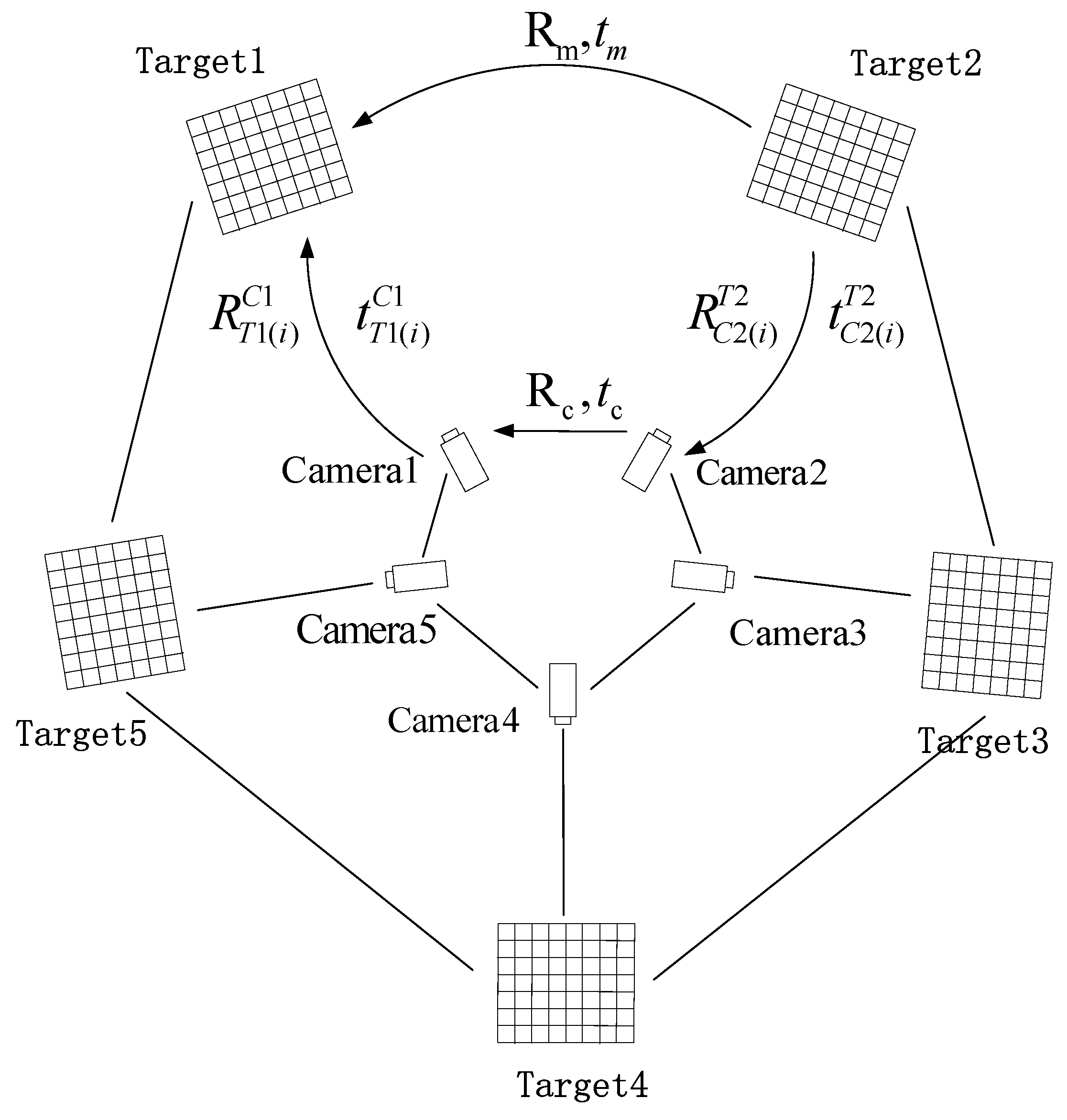
2.2. The Global Optimal Method of Multi-Cameras Calibration
2.2.1. Global Optimization Method of Rotation Matrices in Extrinsic Parameters.
2.2.2. Global Optimization Method of Translation Vector in Extrinsic Parameters.
3. Results
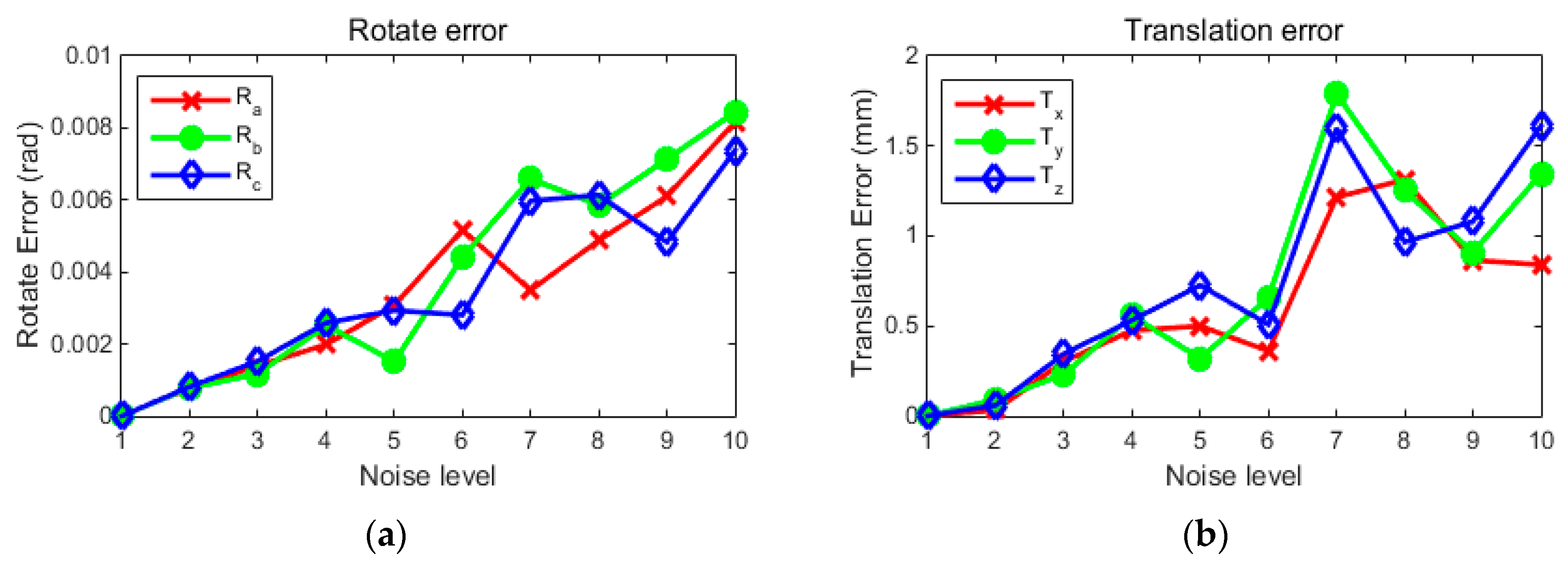
3.1. A Simulation Experiment of Two Cameras
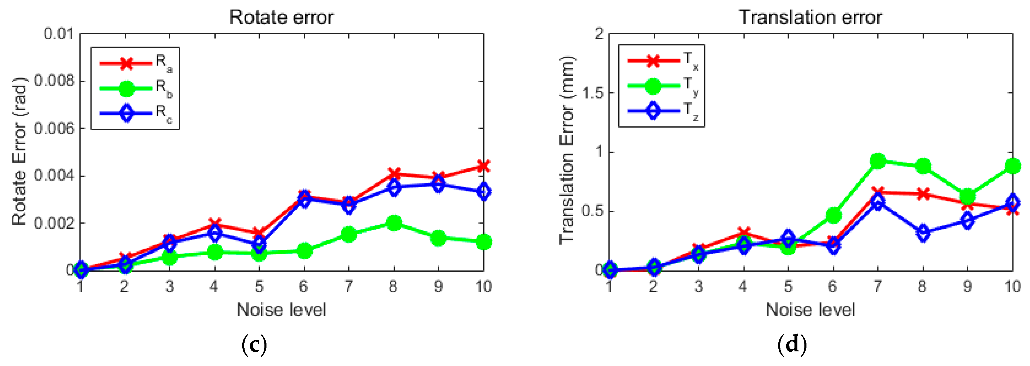
3.2. Simulation Experiment of Multi-Camera Extrinsic Parameters Calibration with the Global Optimization Method
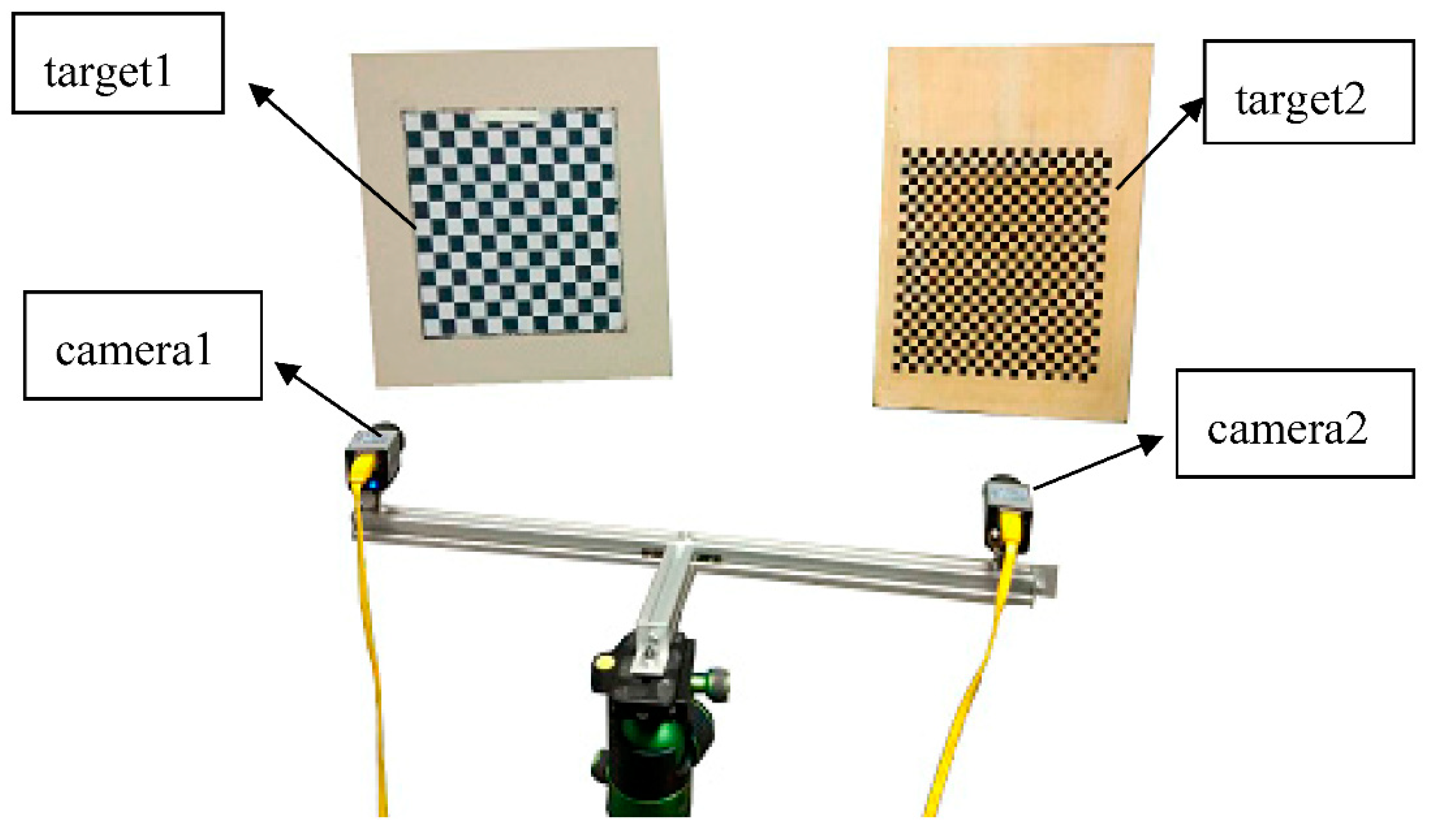
3.3. Two Camera Experiment with Real Image
3.4. Real Data Experiment of Global Optimization Calibration for Multi-Cameras
4. Discussion
5. Conclusions
Author Contributions
Funding
Acknowledgments
Conflicts of Interest
References
- Colomina, I.; Molina, P. Unmanned aerial systems for photogrammetry and remote sensing: A review. ISPRS J. Photogramm. Remote Sens. 2014, 92, 79–97. [Google Scholar] [CrossRef]
- Everaerts, J. The use of unmanned aerial vehicles (UAVs) for remote sensing and mapping. Int. Arch. Photogramm. Remote Sens. Spat. Inf. Sci. 2008, 37, 1187–1192. [Google Scholar]
- Rupnik, E.; Nex, F.; Toschi, I.; Remondino, F. Aerial multi-camera systems: Accuracy and block triangulation issues. ISPRS J. Photogramm. Remote Sens. 2015, 101, 233–246. [Google Scholar] [CrossRef]
- Turner, D.; Lucieer, A.; Watson, C. An automated technique for generating georectified mosaics from ultra-high resolution unmanned aerial vehicle (UAV) imagery, based on structure from motion (SfM) point clouds. Remote Sens. 2012, 4, 1392–1410. [Google Scholar] [CrossRef]
- Mancini, F.; Dubbini, M.; Gattelli, M.; Stecchi, F.; Fabbri, S.; Gabbianelli, G. Using unmanned aerial vehicles (UAV) for high-resolution reconstruction of topography: The structure from motion approach on coastal environments. Remote Sens. 2013, 5, 6880–6898. [Google Scholar] [CrossRef]
- Harwin, S.; Lucieer, A. Assessing the accuracy of georeferenced point clouds produced via multi-view stereopsis from unmanned aerial vehicle (UAV) imagery. Remote Sens. 2012, 4, 1573–1599. [Google Scholar] [CrossRef]
- d’Oleire-Oltmanns, S.; Marzolff, I.; Peter, K.D.; Ries, J.B. Unmanned aerial vehicle (UAV) for monitoring soil erosion in Morocco. Remote Sens. 2012, 4, 3390–3416. [Google Scholar] [CrossRef]
- Dandois, J.P.; Ellis, E.C. Remote sensing of vegetation structure using computer vision. Remote Sens. 2010, 2, 1157–1176. [Google Scholar] [CrossRef]
- Lee, J.J.; Shinozuka, M. A vision-based system for remote sensing of bridge displacement. NDT E Int. 2006, 39, 425–431. [Google Scholar] [CrossRef]
- Zhang, Z. A flexible new technique for camera calibration. IEEE Trans. Pattern Anal. Mach. Intell. 2000, 22, 1330–1334. [Google Scholar] [CrossRef]
- Zhang, Z. Camera calibration with one-dimensional objects. IEEE Trans. Pattern Anal. Mach. Intell. 2004, 26, 892–899. [Google Scholar] [CrossRef] [PubMed]
- Gurdjos, P.; Crouzil, A.; Payrissat, R. Another way of looking at plane-based calibration: The centre circle constraint. In Proceedings of the European Conference on Computer Vision, Copenhagen, Denmark, 28–31 May 2002; Springer: Berlin/Heidelberg, Germany, 2002; pp. 252–266. [Google Scholar]
- Gurdjos, P.; Sturm, P. Methods and geometry for plane-based self-calibration. In Proceedings of the IEEE Computer Society Conference on Computer Vision and Pattern Recognition, Madison, WI, USA, 18–20 June 2003; pp. 491–496. [Google Scholar]
- Tsai, R.Y. An efficient and accurate camera calibration technique for 3D machine vision. In Proceedings of the IEEE Computer Society Conference on Computer Vision and Pattern Recognition, Miami Beach, FL, USA, 22–26 June1986; pp. 364–374. [Google Scholar]
- Tsai, R. A versatile camera calibration technique for high-accuracy 3D machine vision metrology using off-the-shelf TV cameras and lenses. IEEE J. Robot. Autom. 1987, 3, 323–344. [Google Scholar] [CrossRef]
- Agrawal, M.; Davis, L. Complete camera calibration using spheres: A dual space approach. IEEE Int. Conf. Comput. Vis. 2003, 206, 782–789. [Google Scholar]
- Zhang, H.; Zhang, G.; Wong, K.Y. Camera calibration with spheres: Linear approaches. In Proceedings of the IEEE International Conference on Image Processing 2005 (ICIP 2005), Genova, Italy, 14 September 2005; IEEE: New York, NY, USA; p. II-1150. [Google Scholar]
- Gong, Z.; Liu, Z.; Zhang, G. Flexible global calibration of multiple cameras with nonoverlapping fields of view using circular targets. Appl. Opt. 2017, 56, 3122–3131. [Google Scholar] [CrossRef] [PubMed]
- Dong, S.; Shao, X.; Kang, X.; Yang, F.; He, X. Extrinsic calibration of a non-overlapping camera network based on close-range photogrammetry. Appl. Opt. 2016, 55, 6363–6370. [Google Scholar] [CrossRef] [PubMed]
- Xia, R.; Hu, M.; Zhao, J.; Chen, S.; Chen, Y. Global calibration of multi-cameras with non-overlapping fields of view based on photogrammetry and reconfigurable target. Meas. Sci. Technol. 2018, 29, 065005. [Google Scholar] [CrossRef]
- Lu, R.S.; Li, Y.F. A global calibration method for large-scale multi-sensor visual measurement systems. Sens. Actuators A Phys. 2004, 116, 384–393. [Google Scholar] [CrossRef]
- Lébraly, P.; Deymier, C.; Ait-Aider, O.; Royer, E.; Dhome, M. Flexible extrinsic calibration of non-overlapping cameras using a planar mirror: Application to vision-based robotics. In Proceedings of the IEEE/RSJ International Conference on IEEE Intelligent Robots and Systems (IROS), Taipei, Taiwan, 18–22 October 2010; pp. 5640–5647. [Google Scholar]
- Kumar, R.K.; Ilie, A.; Frahm, J.M.; Pollefeys, M. Simple calibration of non-overlapping cameras with a mirror. In Proceedings of the CVPR 2008. IEEE Conference on Computer Vision and Pattern Recognition, Anchorage, AK, USA, 23–28 June 2008; pp. 1–7. [Google Scholar]
- Pagel, F. Extrinsic self-calibration of multiple cameras with non-overlapping views in vehicles. In Proceedings of the International Society for Optics and Photonics, Video Surveillance and Transportation Imaging Applications, San Francisco, CA, USA, 3–5 February 2014; Volume 9026, p. 902606. [Google Scholar]
- Liu, Z.; Wei, X.; Zhang, G. External parameter calibration of widely distributed vision sensors with non-overlapping fields of view. Opt. Lasers Eng. 2013, 51, 643–650. [Google Scholar] [CrossRef]
- Lepetit, V.; Moreno-Noguer, F.; Fua, P. Epnp: An accurate o (n) solution to the PNP problem. Int. J. Comput. Vis. 2009, 81, 155. [Google Scholar] [CrossRef]
- Madsen, K.; Nielsen, H.B.; Tingleff, O. Methods for Non-Linear Least Squares Problems; Informatics and Mathematical Modelling, Technical University of Denmark, DTU: Lyngby, Denmark, 1999; pp. 24–29. [Google Scholar]
- Martinec, D.; Pajdla, T. Robust rotation and translation estimation in multiview reconstruction. In Proceedings of the CVPR’07. IEEE Conference on Computer Vision and Pattern Recognition, Minneapolis, MN, USA, 17–22 June 2007; pp. 1–8. [Google Scholar]
- Jiang, N.; Cui, Z.; Tan, P. A global linear method for camera pose registration. In Proceedings of the 2013 IEEE International Conference on Computer Vision (ICCV), Sydney, Australia, 1–8 December 2013; pp. 481–488. [Google Scholar]
- Camera Calibration Toolbox for Matlab. Available online: http://robots.stanford.edu/cs223b04/JeanYvesCalib/index.html#links (accessed on 5 June 2018).
- Horn, B.K. Closed-form solution of absolute orientation using unit quaternions. JOSA A 1987, 4, 629–642. [Google Scholar] [CrossRef]


| Camera Number | Extrinsic Parameters | |||||
|---|---|---|---|---|---|---|
| Roll Angle (rad) | Yew Angle (rad) | Pitching Angle (rad) | X-Axis Translation (mm) | Y-Axis Translation (mm) | Y-Axis Translation (mm) | |
| 1 | 0 | 0 | 0 | 0 | 0 | 0 |
| 2 | 0.698 | 0.175 | 0.157 | 500 | −100 | 10 |
| 3 | 1.484 | 0.262 | 0.367 | 600 | 300 | −50 |
| 4 | 2.426 | 0.559 | 0.716 | −10 | 600 | 20 |
| 5 | −1.047 | −0.070 | 0.401 | −590 | 400 | 20 |
| Noise Level | Extrinsic Parameters | Camera 2 | Camera 4 | Camera 5 | |||
|---|---|---|---|---|---|---|---|
| Before Optimization | After Optimization | Before Optimization | After Optimization | Before Optimization | After Optimization | ||
| Level 2 | a (rad) | 0.00194 | 0.00135 | 0.00208 | 0.00165 | 0.00183 | 0.00122 |
| b (rad) | 0.00192 | 0.00114 | 0.00210 | 0.00194 | 0.00174 | 0.00116 | |
| c (rad) | 0.00203 | 0.00156 | 0.00199 | 0.00118 | 0.00207 | 0.00095 | |
| x (mm) | 0.103 | 0.064 | 0.121 | 0.071 | 0.104 | 0.063 | |
| y (mm) | 0.089 | 0.077 | 0.009 | 0.069 | 0.009 | 0.054 | |
| z (mm) | 0.101 | 0.068 | 0.110 | 0.078 | 0.100 | 0.077 | |
| Level 5 | a (rad) | 0.00506 | 0.00398 | 0.00400 | 0.00334 | 0.00512 | 0.00265 |
| b (rad) | 0.00513 | 0.00351 | 0.00523 | 0.00416 | 0.00501 | 0.00296 | |
| c (rad) | 0.00498 | 0.00324 | 0.00491 | 0.00359 | 0.00523 | 0.00312 | |
| x (mm) | 0.251 | 0.172 | 0.254 | 0.192 | 0.249 | 0.156 | |
| y (mm) | 0.262 | 0.150 | 0.251 | 0.209 | 0.250 | 0.165 | |
| z (mm) | 0.249 | 0.149 | 0.236 | 0.186 | 0.251 | 0.227 | |
| Parameters | Left Camera | Right Camera |
|---|---|---|
| Focal length/pixel | [2564.60, 2564.09] | [2571.31, 2570.61] |
| Principal point/pixel | [599.75, 492.33] | [625.87, 503.24] |
| Image Distortion coefficients | [−0.436, −0.347, 0.00069, 0.0018, 0] | [−0.456, −0.109, −0.00023, −0.00044, 0] |
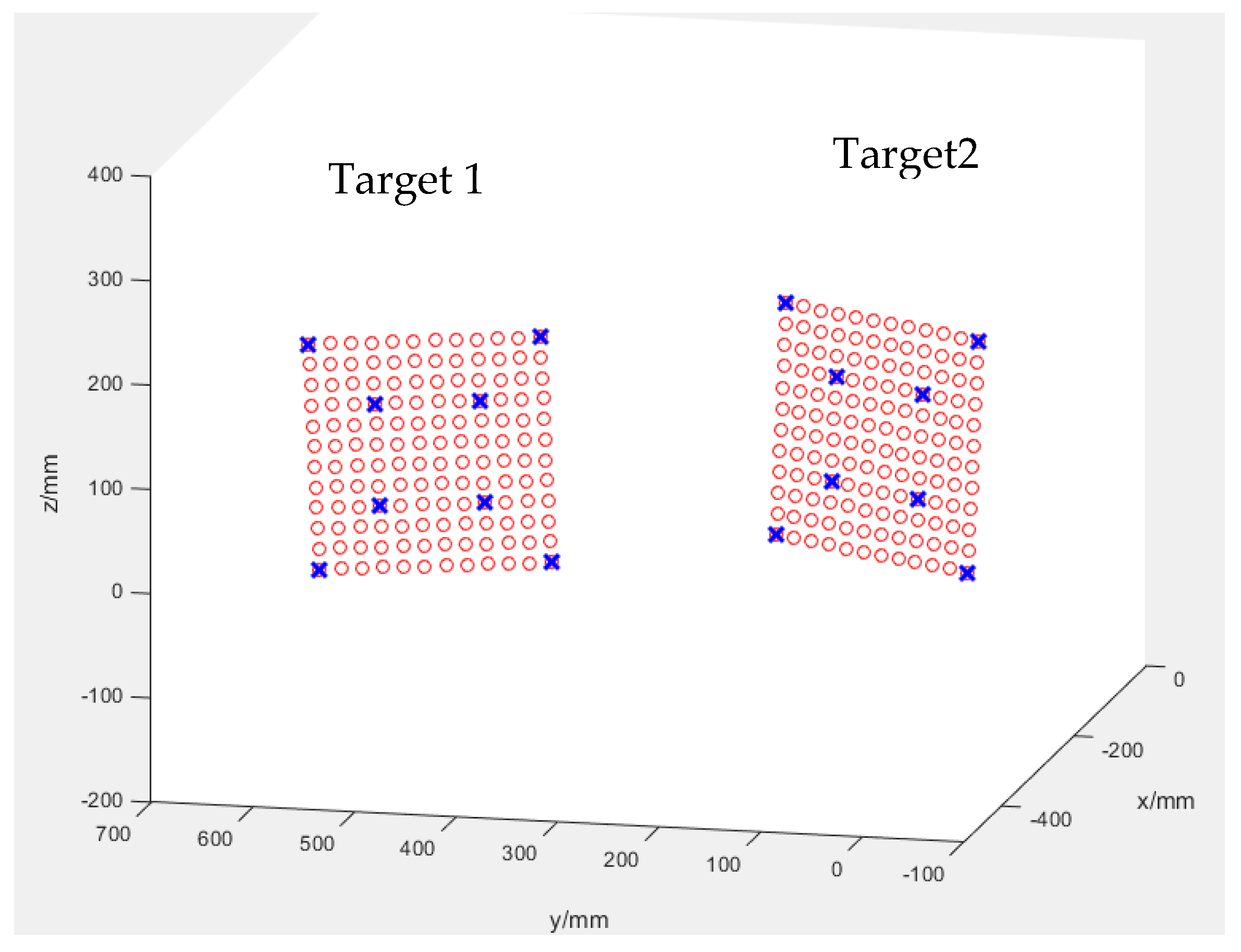
| Points | Target 1 | Target 2 | ||||
|---|---|---|---|---|---|---|
| Index | X/mm | Y/mm | Z/mm | X/mm | Y/mm | Z/mm |
| 1 | −308.693 | 374.455 | −19.030 | −298.538 | −31.703 | −13.293 |
| 2 | −334.978 | 592.731 | −27.055 | −235.764 | 179.053 | −7.990 |
| 3 | −319.212 | 435.772 | 38.660 | −279.511 | 23.678 | 48.073 |
| 4 | −331.265 | 534.998 | 35.012 | −250.941 | 119.475 | 50.494 |
| 5 | −324.809 | 438.777 | 138.458 | −276.212 | 20.179 | 147.967 |
| 6 | −336.763 | 537.993 | 134.810 | −247.634 | 115.978 | 150.378 |
| 7 | −320.996 | 381.044 | 200.526 | −291.380 | −39.398 | 206.452 |
| 8 | −347.291 | 599.319 | 192.504 | −228.510 | 172.059 | 211.754 |
| Rotate | Translation | |||||
|---|---|---|---|---|---|---|
| Index | a (rad) | b (rad) | c (rad) | x (mm) | y (mm) | z (mm) |
| 1 | 0.412535 | −0.073078 | −0.084716 | −165.3740 | −497.73 | −43.4709 |
| 2 | 0.413592 | −0.072140 | −0.084732 | −165.3776 | −497.759 | −43.5122 |
| 3 | 0.414233 | −0.072867 | −0.084769 | −165.4139 | −497.785 | −43.4713 |
| 4 | 0.413808 | −0.072550 | −0.085103 | −165.4118 | −497.771 | −43.4689 |
| 5 | 0.412850 | −0.072154 | −0.084903 | −165.3968 | −497.78 | −43.5357 |
| 6 | 0.413207 | −0.072816 | −0.085246 | −165.3841 | −497.77 | −43.5158 |
| 7 | 0.413391 | −0.072739 | −0.085004 | −165.3767 | −497.757 | −43.5191 |
| 8 | 0.414433 | −0.072085 | −0.085072 | −165.3915 | −497.75 | −43.4718 |
| 9 | 0.412782 | −0.072789 | −0.085163 | −165.3668 | −497.756 | −43.4529 |
| 10 | 0.4141816 | −0.071671 | −0.08515 | −165.3728 | −497.723 | −43.5063 |
| 11 | 0.413759 | −0.071354 | −0.085006 | −165.3578 | −497.751 | −43.4597 |
| 12 | 0.413222 | −0.071859 | −0.085203 | −165.3841 | −497.717 | −43.471 |
| 13 | 0.412851 | −0.072632 | −0.084900 | −165.3964 | −497.742 | −43.5423 |
| 14 | 0.413326 | −0.072151 | −0.084977 | −165.4096 | −497.716 | −43.4788 |
| 15 | 0.413434 | −0.073104 | −0.084842 | −165.3793 | −497.773 | −43.5017 |
| truth values | 0.41347 | −0.07232 | −0.08496 | −165.391 | −497.746 | −43.524 |
| std | 0.000546 | 0.000527 | 0.000172 | 0.01679 | 0.02255 | 0.02860 |
| Camera Number | The Maximum Value of the Errors | |||||
|---|---|---|---|---|---|---|
| a (rad) | b (rad) | c (rad) | x (mm) | y (mm) | z (mm) | |
| Camera 3 | 0.000921 | 0.000894 | 0.000565 | 0.066 | 0.059 | 0.078 |
| Camera 4 | 0.000945 | 0.000818 | 0.000632 | 0.071 | 0.062 | 0.077 |
© 2018 by the authors. Licensee MDPI, Basel, Switzerland. This article is an open access article distributed under the terms and conditions of the Creative Commons Attribution (CC BY) license (http://creativecommons.org/licenses/by/4.0/).
Share and Cite
Yin, L.; Wang, X.; Ni, Y.; Zhou, K.; Zhang, J. Extrinsic Parameters Calibration Method of Cameras with Non-Overlapping Fields of View in Airborne Remote Sensing. Remote Sens. 2018, 10, 1298. https://doi.org/10.3390/rs10081298
Yin L, Wang X, Ni Y, Zhou K, Zhang J. Extrinsic Parameters Calibration Method of Cameras with Non-Overlapping Fields of View in Airborne Remote Sensing. Remote Sensing. 2018; 10(8):1298. https://doi.org/10.3390/rs10081298
Chicago/Turabian StyleYin, Lei, Xiangjun Wang, Yubo Ni, Kai Zhou, and Jilong Zhang. 2018. "Extrinsic Parameters Calibration Method of Cameras with Non-Overlapping Fields of View in Airborne Remote Sensing" Remote Sensing 10, no. 8: 1298. https://doi.org/10.3390/rs10081298
APA StyleYin, L., Wang, X., Ni, Y., Zhou, K., & Zhang, J. (2018). Extrinsic Parameters Calibration Method of Cameras with Non-Overlapping Fields of View in Airborne Remote Sensing. Remote Sensing, 10(8), 1298. https://doi.org/10.3390/rs10081298