Abstract
Forests in the Southwestern United States are becoming increasingly susceptible to large wildfires. As a result, forest managers are conducting forest fuel reduction treatments for which spatial fuels and structure information are necessary. However, this information currently has coarse spatial resolution and variable accuracy. This study tested the feasibility of using unmanned aerial vehicle (UAV) imagery to estimate forest canopy fuels and structure in a southwestern ponderosa pine stand. UAV-based multispectral images and Structure-from-Motion point clouds were used to estimate canopy cover, canopy height, tree density, canopy base height, and canopy bulk density. Estimates were validated with field data from 57 plots and aerial photography from the U.S. Department of Agriculture National Agriculture Imaging Program. Results indicate that UAV imagery can be used to accurately estimate forest canopy cover (correlation coefficient (R2) = 0.82, root mean square error (RMSE) = 8.9%). Tree density estimates correctly detected 74% of field-mapped trees with a 16% commission error rate. Individual tree height estimates were strongly correlated with field measurements (R2 = 0.71, RMSE = 1.83 m), whereas canopy base height estimates had a weaker correlation (R2 = 0.34, RMSE = 2.52 m). Estimates of canopy bulk density were not correlated to field measurements. UAV-derived inputs resulted in drastically different estimates of potential crown fire behavior when compared with coarse resolution LANDFIRE data. Methods from this study provide additional data to supplement, or potentially substitute, traditional estimates of canopy fuel.
Keywords:
unmanned aerial vehicle (UAV); drone; wildfire; fire behavior; structure-from-motion; SfM; lidar; base height; bulk density; cover 1. Introduction
The Southwestern United States is home to the largest contiguous ponderosa pine (Pinus ponderosa) forest in the world [1,2]. The southwestern ponderosa pine forests serve an ecologically important role by providing biodiversity, wildlife habitat, carbon storage, and sequestration functions, as well as ecosystem services for the surrounding communities. In these forests, fire suppression, heavy grazing, logging, and climate change have created increased susceptibility to high-intensity crown fires, putting the forest ecosystems and neighboring communities at risk [1,3,4,5]. Historically, southwestern forests experienced frequent low-intensity fires that consumed forest fuels and effectively thinned younger trees to maintain a low tree density. Euro-American settlement brought changes in land use and introduced fire suppression, which removed this natural balancing mechanism [6,7]. The forests that were naturally maintained by frequent low-intensity fires are now characterized by an overabundance of forest fuel [8,9,10,11].
The U.S. Forest Service is implementing large-scale forest fuel reduction treatments across the state of Arizona to reduce the risks of catastrophic fires. Such forest fuel reduction treatments often include a combination of mechanical thinning followed by the reintroduction of periodic low-intensity fire. Forest thinning is designed to manipulate forest structure, such as canopy cover, canopy height, crown base height, and crown bulk density, to produce forest conditions within the natural range of variability [12,13,14,15]. Reintroduction of low-intensity fire is used to restore the natural fire regime and maintain a balance of forest fuels [16,17]. These techniques can decrease the risk of wildfire, reduce the impacts of wildfire, reduce outbreaks of insects and disease, and help mitigate the effects of a changing climate [4,5,18,19,20,21].
Land managers often use detailed spatial forest structure information when planning, implementing, and monitoring forest fuels treatments. Currently, most fuels treatment efforts use spatial fuel information from the Landscape Fire and Resource Management Planning Tools Project (LANDFIRE) database, which is an interagency partnership primarily between the United States Department of Agriculture (USDA) Forest Service and the United States Department of Interior (DOI). LANDFIRE provides comprehensive nationwide coverage across the U.S., is updated every two–five years, and is available for free (www.landfire.gov). The spatial fuels products provided by the LANDFIRE project include: canopy cover, canopy height, crown base height, crown bulk density, and fire behavior fuel models. However, its 30 m spatial resolution is too coarse to represent the variations in forest fuel at a local scale [22] and LANDFIRE data applications are limited to landscape scales only (>405 hectares) [15,23,24]. Finer resolution data that accurately represent local-scale forest characteristics are needed to generate more detailed wildfire models. The accuracies in the LANDFIRE forest fuels raster products can vary by location compared to field-based measurements and often need to be adjusted to better represent actual site-specific conditions [25]. For example, in a study conducted by Reeves et al. [26] across 12 different sites, LANDFIRE canopy base heights had correlation coefficient (R2) values that ranged from 0 to 0.93 when compared to field data.
Recent developments in unmanned aerial vehicles (UAVs) and miniaturization of sensor technologies have made them an attractive alternative for acquiring high resolution data at local scales. Compared to the resolution of aerial images (one meter resolution) or satellite data (2–30 m resolution), images acquired from UAVs tend to have spatial resolutions of 5–15 cm due to a lower altitude of acquisition. Additionally, UAVs offer the ability to control the image acquisition process and timing, and can obtain overlapping images to the user’s specifications. Similar to aerial- and satellite-based spectral data, UAV images can be used for classifying vegetation types and estimating forest canopy cover [27,28,29,30]. If acquired with high overlap, UAV images can be used with Structure-from-Motion (SfM) algorithms to produce three-dimensional (3D) point cloud data that represent both the ground surface and vegetation [31,32], which can then be used to derive forest structure information. Currently, UAV SfM datasets have a smaller footprint (40–120 hectares) than aerial lidar, but have finer resolution (10+ points/m2) due to the interpolated nature of the points. Relative to aerial lidar acquisitions, the cost of UAV equipment (roughly around $30,000 for UAV and sensor) enables landowners and managers to purchase their own and conduct surveys as needed. The average cost to conduct a field-based forest inventory is $104–180/plot [33] and field-based surveys are often implemented at a sampling frequency of one plot for every two–three hectares. UAVs can offer more comprehensive coverage and a less human-biased assessment of forest structure characteristics [34], leading to adaptive management opportunities and more informed decision-making.
UAV SfM data (14+ points/m2) have been successfully used in temperate deciduous forests to derive forest canopy height estimations (R2 = 0.86, root mean square error (RMSE) = 3.6 m) [32,35]. When compared against manned airborne lidar data and field measurements, UAV data in a dry sclerophyll eucalypt forest performed well at estimating total canopy cover and tree density, with 82% and 90% detection, respectively, with a R2 of 0.68 (RMSE = 1.3 m) for tree height estimates [36]. UAV-derived estimates for Lorey’s mean height, dominant height, stem numbers, basal area, and stem volume have demonstrated R2 values of 0.71, 0.97, 0.60, 0.60, and 0.85, respectively, with RMSE values of 1.4 m, 0.7 m, 538.2 ha, 4.5 m2/ha, and 38.3 m3/ha, respectively [34]. In Australia, UAV image-derived individual tree segmentation detected 70% of the dominant trees, and 35% of suppressed trees, but with a low R2 of 0.15 in aboveground biomass estimates [37]. Sankey et al. [30] successfully estimated canopy cover (R2 = 0.74; RMSE = 8.5%), individual tree height (R2 of 0.64 to 0.93; RMSE = 1.5 m to 2.9 m), and crown diameter (R2 of 0.66 to 0.70; RMSE of 0.72 to 1.9 m) in a ponderosa pine forest area similar to this study. However, the individual tree delineation showed weaker correlations with field-based measurements (R2 of 0.36–0.53; RMSE of 0.83 trees/100 m2 and 2.2 trees/100 m2) [30]. Our study tested the accuracies in measuring tree canopy base height and canopy bulk density using SfM methods. At the time of this study, no others had tested and quantified the accuracy of canopy base height and bulk density using these methods.
Our overall goal was to estimate ponderosa pine forest canopy fuel and potential crown fire behavior using UAV data to supplement the coarse-resolution LANDFIRE data and better represent actual site-specific conditions. The specific objectives included the following:
- Estimate the following stand-level variables from the UAV data in 10 m cells for fire behavior modeling: total canopy cover (%), tree density (total no./cell), mean canopy height (m), mean canopy base height (m), mean canopy bulk density (kg/m3), topographic elevation (m), slope (degrees), and aspect (azimuth).
- Test and quantify the errors associated with UAV SfM-derived point cloud data in delineating individual trees and estimating for each individual tree: total height, canopy base height, and canopy bulk density.
If successfully generated, these UAV-based data could offer a fuel measurement method that is more efficient and potentially more accurate than field surveys. By supplementing or replacing LANDFIRE data, UAV-derived metrics can provide fine- to mid-scale spatial data and provide opportunities for managers to prioritize treatments, calibrate ongoing treatments, and conduct responsive adaptive management.
2. Materials and Methods
2.1. Study Area
This study focused on the wildland-urban interface of Flagstaff, Arizona, USA, and the surrounding Coconino National Forest managed by the U.S. Forest Service (Figure 1). Specifically, we focused on a 12.14 ha area that has been identified by the city of Flagstaff as high priority for fuels treatment and mechanical thinning, due to its close proximity to residential structures, and is located in Phase 1 of a forest fuels reduction project known as the Flagstaff Watershed Protection Project (FWPP). The study area has not experienced any timber harvesting since 1970 and was chosen due to its operational feasibility for UAV use. Phase 2 of FWPP is also located in Coconino National Forest and includes helicopter and skyline cable harvesting techniques, which is planned to be treated in future years. The final treatment area, Phase 3, is located about 25 km southeast of Flagstaff.
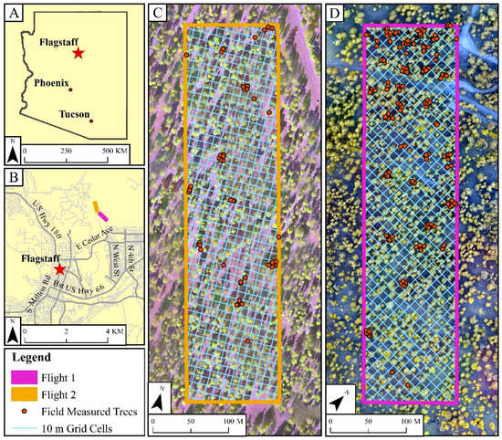
Figure 1.
Vicinity map of our study site, UAV flight areas, and field sampling locations: (A) Location of our study area in within the state of Arizona, (B) UAV flight locations and their proximity to Flagstaff, Arizona, USA, and (C, D) Both UAV flight areas overlaid on false color UAV imagery with points representing each field measured tree.
The elevation of the study area ranges between 2158 and 2188 m above sea level with a southwest aspect of 0–10 degrees slope. Annual mean precipitation is 55 cm, which predominantly occurs during summer Monsoon events and winter snowfall, and the mean annual temperature is 7.9 °C. On average, the coolest month is December, with an average temperature of −1.3 °C, whereas July is the warmest month with an average temperature of 18.9 °C [38]. The dominant overstory vegetation type is ponderosa pine (Pinus ponderosa) with a small Gambel oak (Quercus gambelii) component. Native understory vegetation is primarily composed of Arizona fescue (Festuca arizonica), bottlebrush squirreltail (Elymus elymoides), mountain muhly (Muhlenbergia montana), and Fendler’s ceanothus (Ceanothus fendleri). Common invasive species in this area include Dalmatian toadflax (Linaria dalmatica), common mullein (Verbascum thapsus), and cheatgrass (Bromus tectorum).
2.2. UAV Images and Pre-Processing
We used a SenseFly eBee fixed-wing UAV platform that weighs approximately 537 g with a wingspan of 96 cm [30,34]. The fixed-wing UAV has a cruising speed of 40–90 km/h and maximum flight coverage of 12 km2 under optimal conditions [39]. It is launched by hand and lands by reducing speed and altitude until it belly lands. The eBee operates with eMotion 2 [40] custom flight planning software package and a ground station, which sends waypoint navigation data to the aircraft to perform pre-planned, autonomous flights. We completed two UAV surveys on 21 August 2016 and on 22 November 2016 close to solar noon to minimize shadowing (Figure 1). The temporal difference between the two survey dates had minimal impact at our study site, which is dominated by evergreen conifer trees. Both surveys were conducted with 85–90% latitudinal and longitudinal overlap, at a maximum flight altitude of 120 m, resulting in image pixel resolution of 15 cm. Flight 1 lasted for 15 min resulting in 960 individual images taken, whereas Flight 2 took 22 min to complete and acquired a total of 1828 individual images.
The eBee UAV was equipped with a multispectral sensor with four spectral bands: green (550 nm), red (660 nm), red edge (735 nm), and near-infrared (790 nm). The images were processed using Pix4D software (Pix4D, Lausanne, Switzerland), which effectively co-registers and merges the images together to create an orthomosaic image for each spectral band. The resulting four orthomosaics were then spectrally stacked with ENVI 5.3 (Harris Geospatial Solutions, Broomfield, CO, USA) image analysis software to create a single multispectral orthomosaic image with the four separate bands with 15 cm spatial resolution for each flight area.
We also generated 3D point cloud data using the Pix4D software from each spectral band and merged them in CloudCompare (www.cloudcompare.org) software to create a single, dense point cloud file for each flight area. The average point densities for the point clouds were 32 points/m2 and 56 points/m2 for Flights 1 and 2, respectively. The point cloud for Flight 2 contained a few spurious points that were well below the ground height, which were removed using the Statistical Outlier Removal tool in CloudCompare software with one standard deviation.
2.3. UAV Image-Derived Canopy Cover
Forest canopy cover was derived using the UAV orthomosaic images and a normalized difference vegetation index (NDVI)-based segmentation method. First, NDVI was calculated in ENVI 5.3 software with the following equation:
Our preliminary tests indicated that the NIR and red edge band combination generated a better NDVI raster than the NIR and red band combination with the images from our sensor. Next, the ENVI image segmentation tool was used to classify canopy pixels, which were then overlaid on a canopy height model raster, generated with the raster (https://CRAN.R-project.org/package=raster) package in R (R Development Core Team 2008, Vienna, Austria), to remove pixels with a tree canopy height of less than 1.37 m. This process effectively removed areas of high NDVI values and low canopy height (e.g., herbaceous vegetation) to produce a raster image of only tree canopy. The resulting binary canopy raster was resampled from 15 cm to 20 cm pixels and imported to ArcMap 10.4 (ESRI 2015, Redlands, California, USA), and summarized into 10 m cells (N = 2500 pixels per 10 m cell) to estimate total canopy cover within each 10 m cell.
The UAV image-derived canopy cover estimates were validated using two different independent data sources. First, the latest available U.S. Department of Agriculture National Agriculture Imagery Program (NAIP) image from summer of 2017 with 1 m spatial resolution was used. A similar workflow to the UAV processing was used to classify canopy cover in the NAIP imagery and summarize the data into 10 m grids (N = 100 NAIP image pixels per 10 m cell). A pixel-wise regression analysis was then used to compare the tree canopy cover estimates from the UAV image classification and NAIP image classification. Secondly, our field-based measurements were used to validate the UAV image-derived canopy cover estimates. Field measurements of each tree canopy diameter were summarized in ArcMap 10.4 to estimate total canopy cover within each 10 × 10 m field plot (N = 57 plots) and compared to UAV image-derived estimates also via a simple linear regression.
2.4. UAV Image-Derived Individual Tree Segmentation
Ground points were first classified in the UAV SfM-derived point cloud data using a progressive morphological filter [41] in the lidR (https://CRAN.R-project.org/package=lidR) package in R. A digital terrain model (DTM) was then created from the ground points and subtracted from the point cloud Z values to calculate above ground height or Z values [34,42,43,44,45]. The resulting point clouds contained an abnormal amount of noise points that were a few meters above the ground surface, but represented neither ground nor vegetation. To remove these points, we applied a second progressive morphological ground filter with a higher maximum threshold height (4 m). Next, the point clouds were overlaid with the NDVI raster image and all points with a NDVI value <0 were excluded. Applying these two steps generated a point cloud that best represented only tree points, which were then used in the tree segmentation algorithm (Figure 2).
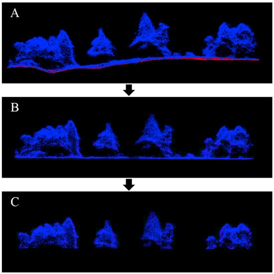
Figure 2.
Point cloud pre-processing prior to tree segmentation: (A) Point cloud with initial ground classification are displayed in red, (B) Point cloud that has been normalized and filtered to remove ground points, which still included some non-tree points, and (C) The final point cloud after the second ground filtering and NDVI threshold only included tree points.
The tree segmentation method in the R lidR package used in this study segments trees by analyzing points from the tree top to bottom and using the horizontal distance between points to determine if they are part of a specific tree [42]. The segmentation method relies on four user-defined parameters: minimum height of a tree, maximum crown radius, and two numeric distances, which define horizontal distance (in meters) thresholds between all points above 15 m in height, and below 15 m in height. These thresholds values are hereafter referred to as distance thresholds (DT). The DT value is site specific [42]. A low DT value generally results in over-segmentation with many additional trees identified in the point cloud, whereas a high DT value causes under-segmentation, where many tree canopies are merged together into single large canopies. In this study, 16 different iterations of varying DT values were tested. We used a minimum tree height of 2 m, and a maximum canopy diameter of 7 m, based on the ranges observed in our field data.
The UAV SfM point cloud-derived trees were first overlaid with the 10 × 10 m grid to count all trees detected within each cell, and then compared to the field-mapped trees to assess the accuracy of the tree segmentation and to quantify true positive detection and false negatives (omissions). False positives (commissions) were calculated by summing the number of UAV point cloud-derived trees within the 10 × 10 m plots that did not match a field-mapped tree. Tree segmentation with constant parameters across the entire study area yielded varying accuracies in areas of higher versus lower tree density. Assuming a linear relationship between tree density and canopy cover, an optimized version of the tree segmentation was developed. Using the UAV image-derived tree canopy cover estimates, we first classified the study area into regions of high canopy cover and low canopy cover. In areas of >50% canopy cover, the tree points from a lower DT value iteration were used, and in areas of <50% canopy cover, the tree points from a higher DT value iteration were used.
Validation metrics used to assess each tree segmentation iteration included recall (r), precision (p), and F-score (F), which were calculated using the following equations [42,46]:
Additionally, an ANOVA test with Tukey’s multiple comparisons was conducted to determine if a statistically significant different number of trees were detected between the UAV point cloud data and field-based measurements within each density class and between the UAV point cloud-derived density estimates among different density classes.
2.5. UAV Image-Derived Individual Tree Metrics
The following individual tree measurements were derived from the UAV SfM point cloud data: the X and Y coordinates of each tree top, canopy diameter, total tree height, canopy base height, canopy bulk density, and percentile heights (ranging from 5th to 99th percentiles in 5 m increments). These metrics were compared to the corresponding field-mapped trees for validation: total tree height, canopy base height, and canopy bulk density. Several possible UAV-derived predictor variables were explored to estimate canopy base height and canopy bulk density. For canopy base height, these predictor variables included the height percentiles of each segmented tree and the height-to-crown-diameter ratio. Estimates for canopy bulk density involved first establishing a tree height to diameter at breast height (DBH) relationship. This relationship was used to predict tree DBH with the UAV-derived tree height. The predicted DBHs were then used in northern Arizona-specific allometric equations, shown in Equations (5)–(7), for ponderosa pine [47] to estimate the canopy mass of each tree. The UAV-derived total tree height, average canopy radius, and canopy base height were then used to estimate canopy volume assuming a cylindrical canopy model. Canopy mass was then divided by canopy volume to estimate the canopy bulk density. This process for estimating canopy bulk density directly mirrored the steps used with the field measurements to estimate bulk density. Linear regression models then were used to examine the relationships between the UAV image-derived and field-measured variables. A bootstrap resampling analysis (subsample = 100; iterations = 100,000) was conducted with the UAV tree height measurement errors to determine the mean error with a 90% confidence interval.
2.6. Field Validation
Field measurements were designed to provide a validation dataset for the forest stand characteristics and individual tree measurements derived from the UAV data. Two specific forest stand-level variables that required validation data were: tree canopy cover and tree density estimates in 10 m cells (100 m2). Using 10 m grids in ArcMap, along with polygons of the study areas imaged with the UAV, we first randomly chose 100 field plot locations with a minimum distance of 10 m (Figure 1). Field sampling was then stratified by tree density based on an initial visual estimate of tree density (trees/cell) in the high-resolution (~15 cm) orthomosaic image from the UAV surveys. The study area contained only a few areas of higher tree density, but the desired goal of this study was to measure and evaluate tree canopy cover and tree density estimates across the entire possible range of tree densities (1–7 trees/cell). We, therefore, actively sought and located at least 5 cells with higher densities of 5, 6, and 7 trees/cell, and at least 10 cells with a lower density of 1 to 4 trees/cells (Table 1). The sampling goal was achieved at all density levels with a total 57 plots, 10 × 10 m in dimension, distributed across the study area. We then navigated to the four corners of each plot to match the locations of the field plots with the 10 m cells derived in ArcMap 10.4. Once the plot boundaries were delineated, the global positioning system (GPS) location of each tree inside the plot was digitized on the orthomosaic map to ensure that matching area and individual trees were examined in the field and UAV images.

Table 1.
Distribution of the field samples. Field sampling was stratified by tree density to collect individual tree measurements in areas of varying density. The sampling goal was to measure 10 cells with a density of 1, 2, 3, and 4 trees/cell, and 5 cells with a density of 5, 6, and 7 trees/cell. The sampling goal was met at all densities.
To validate the UAV-derived individual tree metrics, the following measurements were made for every tree within each field plot: species identification, diameter at breast height (DBH), canopy diameter in the north–south and east–west axes, total tree height, canopy base height, and canopy bulk density. The DBH was measured using a diameter tape at a height of 1.37 m on the upslope side of the tree. Canopy diameter was measured using a Leica DISTO E7500i laser rangefinder (Leica Geosystems, St Gallen, Switzerland) in both the north–south and east–west axes, which were determined using a Suunto MC2 compass (Suunto, Vantaa, Finland) with 10° E magnetic declination adjustment. Canopy height and canopy base height were measured using the laser rangefinder to determine horizontal distance to the tree, and a Suunto PM-5 (Suunto, Vantaa, Finland) clinometer to measure the angles to tree base, canopy top, and canopy base. Canopy base was the lowest point of the continuous canopy. The distance and angle measurements were then used to calculate tree height and canopy base height. Canopy bulk density was calculated by first estimating canopy mass using DBH and allometric equations, shown in Equations (5)–(7), by Kaye et al. [47]. The canopy volume was then calculated using the average canopy radius, overall tree height, and canopy base height, assuming a cylindrical canopy model, as shown in Equation (8). Crown mass was divided by crown volume to estimate a crown bulk density for each tree, given by Equation (9).
2.7. Fire Behavior Modeling
Land managers typically use spatial fuels data from LANDFIRE with FlamMap 5 [48] (U.S. Forest Service Rocky Mountain Research Station, Missoula, Montana, USA) to model potential fire behavior in an area of interest. We compared some of the LANDFIRE variables and UAV image-derived variables as inputs to FlamMap 5 software to model crown fire behavior and to determine if a different image source and resulting input rasters would produce substantially different fire behavior models. FlamMap is used to combine forest fuel characteristics, topography, fuel moisture, and weather factors to model fire behavior outputs. The outputs include flame length in meters, rate of spread in meters per minute, and potential crown fire activity. Using FlamMap with LANDFIRE and UAV image-derived input variables, we estimated areas of surface, passive crown, or active crown fire. Surface fire is defined as a fire burning through the fuels on the ground surface. Passive crown fire occurs in an area that exhibits surface fire and contains a canopy base height low enough to initiate crown fire, but the canopy bulk density is insufficient to carry the crown fire. Active crown fire occurs where crown fire initiation is achieved and canopy bulk density can adequately carry a crown fire [49,50].
The spatial fuels products produced in 30 m cells by the LANDFIRE project include: canopy cover, total canopy height, crown base height, crown bulk density, and fire behavior fuel models. Canopy height describes the average height of the forest canopy within a 30 m grid cell [26]. Crown bulk density is the mass of canopy fuel per canopy volume that would burn in a crown fire [51,52,53]. Crown base height is the lowest point at which sufficient canopy fuel exists for ignition (≥0.012 kg/m3) [23]. The fire behavior fuel models refer to the 13 Anderson Fire Behavior Fuel Models [54] and the 40 Scott and Burgan Fire Behavior Fuel Models [55], which describe surface fuel composition and associated fire behavior [56]. These LANDFIRE products are derived from satellite imagery, biophysical gradients, and vegetation structure and composition data, as well as 40 different predictor variables, such as annual precipitation, temperature, evaporation, evapotranspiration, and others [57,58,59,60,61].
The UAV-based canopy height raster was generated by creating a 0.25 m mean canopy height model across the study area that was then resampled to 10 m resolution and classified into 10 m height classes, similar to the LANDFIRE data format. A canopy base height raster was created by using the percentile height of points within each 10 m cell that was the best indicator of field-measured canopy base heights, and reclassified to units used in LANDFIRE (base height in meters × 10). We also used the above described UAV-based canopy cover raster in 10 m resolution as an input to FlamMap. The UAV image-derived DEM in ENVI LiDAR 5.3 (Harris Geospatial Solutions, Broomfield, CO, USA) with 1 m resolution was used to create the elevation, slope, and aspect rasters in ArcMap 10.4. We resampled all three topographic raster layers to 10 m resolution to match all the other raster layers. A previous study assessed the accuracies from the same UAV platform and sensor in a similar area in Northern Arizona [30] and reported that UAV SfM derived DEMs were well correlated to those derived from both terrestrial and UAV-based laser scanning (R2 = 0.71 and 0.73, RMSE = 0.17 m and 0.5 m, respectively). Canopy bulk density was estimated with UAV data, but was not used due to its poor correlation to field-based estimates. Instead, we used the LANDFIRE canopy bulk density raster. Additionally, the fuel model raster was not estimated using UAV data and was also used directly from the LANDFIRE database.
Crown fire behavior models were then performed using combinations of LANDFIRE and UAV data (Table 2). A sensitivity analysis was conducted by substituting one LANDFIRE raster input at a time with a single UAV-derived raster for each iteration to determine the effects of using UAV-derived layers for each input. All FlamMap iterations were conducted using 10 m resolution input raster layers. Since LANDFIRE data have 30 m resolution, the data were resampled to 10 m to be compatible with the UAV data. Additional parameters in FlamMap for modeling crown fire behavior include a fuel moisture file, wind speed, and wind direction. These additional parameters remained constant across all iterations (Table S1).
Table 2.
Inputs rasters used in FlamMap to model crown fire behavior. The outputs from these iterations were then compared to assess the differences in fire behavior models with the UAV-derived inputs (UAV) versus LANDFIRE-based inputs (LF). All LANDFIRE data used were from the 2012 version. All raster input files were either resampled from LANDFIRE 30 m, or resampled from original UAV data resolution, to a matching resolution of 10 m. Iteration 1 modeled crown fire behavior using 30 m LANDFIRE data, Iteration 2 used LANDFIRE data resampled to 10 m. Iterations 3 to 6 tested UAV-derived rasters for topography, canopy cover, canopy height, and canopy base height, respectively. Iteration 7 used all available UAV-derived rasters.
3. Results
3.1. Forest Stand-Level Metrics
The fixed-wing UAV orthomosaic images from Flights 1 and 2 covered 6.7 ha area each with corresponding 3D point cloud data. When an equal number of 10 m cells (N = 1371) from the UAV- and NAIP-derived canopy cover estimates were compared, the regression model resulted in an adjusted R2 of 0.72 (RMSE = 10.91%; Figure 3). The regression coefficients indicated that the NAIP-derived canopy cover estimates were higher than the UAV-derived estimates, especially in areas of high canopy cover (Figure 3). When the UAV image-derived canopy cover estimates were compared to the field plots (N = 57), the regression model also showed a positive correlation (adj. R2 = 0.67, RMSE = 11.87%). In this comparison, the UAV image-derived estimates tended to be lower than the field-based estimates, especially in areas of high canopy cover.
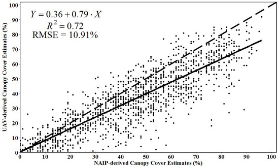
Figure 3.
Regression relationship between the UAV- and NAIP-derived canopy cover estimates with 10 m resolution. The dashed line represents the 1:1 line, and the solid line is the fitted linear regression line.
The UAV SfM point cloud-derived tree density estimates were first compared with field-based measurements in each density class. The mean number of segmented trees for plots with one, two, and three trees closely matched the number of trees mapped in the field plots. However, plots with five, six, and seven trees had a greater variance around the mean estimates. The ANOVA test with Tukey’s multiple pairwise comparisons among the mean segmented trees between all density classes indicated that there was no significant difference between any adjacent density classes. However, UAV point cloud-derived density class 1 contained a significantly different mean number of segmented trees than density classes three, four, five, six, and seven. Density class two had significantly different mean number of segmented trees compared to density class six and seven. Mean segmented trees were not significantly different between density classes two, three, four, and five. Additionally, tree density classes three to seven were not significantly different.
Tree detection was assessed for each DT iteration (Table 3). The iteration with the smallest DT value had the highest detection of 88% or 159 of the 192 field-mapped trees. It also produced the highest commission error with 132 additional trees. The largest DT value had the lowest detection rate (109 of 192 trees), but also the lowest commission error (8 trees). The lowest DT value also had the lowest recall and the highest precision, whereas the highest DT value resulted in the highest recall and lowest precision (Table 3). The highest F-scores occurred with a mid-to-high range of DT values of 1.4 and 1.7 m (0.78). In general, the detection rate decreased as the tree density increased, with lowest detection rates of less than 50% in density classes five, six, and seven. The optimized iteration contained a similarly high F-score of 0.78 and a balance of omission error and commission error was achieved for lower and higher density classes (Table 3).
Table 3.
Individual tree detection results for each iteration. A total of 192 trees were detected. The distance threshold (DT) value was changed by 0.1 m for each iteration to determine the effects of the parameter. The optimized iteration contains two DT values: 1.4 m for areas with more than 50% canopy cover, and 1.7 m for areas of 50% or less canopy cover. Recall (r), precision (p), and F-score (F) are standardized measures of detection, omission, and commission, respectively, calculated with Equations (2)–(4), respectively.
3.2. Individual Tree Metrics
The comparison between the UAV-derived and field-based individual tree metrics was conducted only for the trees that were correctly detected with the optimized DT iteration (N = 142), since this validation required field measurements for every UAV-derived tree. A regression model of UAV-derived tree heights and field-measured tree heights indicated a positive correlation with an adjusted R2 of 0.71 (RMSE = 1.83 m) (Figure 4). A bootstrap resampling analysis with 10,000 iterations indicated that the mean error rate of the UAV-derived tree height was 5.29% of the field measured heights (Table 4).
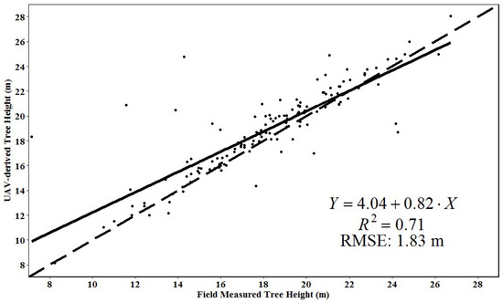
Figure 4.
Linear regression model between the UAV image-derived and field-measured individual tree heights. The solid line represents the fitted regression line and the dashed line is a 1:1 line for reference.
Table 4.
Results comparing UAV-derived and field-derived individual tree metrics. R2, p-value, and RMSE were calculated by linear regression. The mean percent error and range of percent error were calculated using a bootstrap resampling analysis with the percent error between UAV-derived and field-derived estimates.
When all height percentiles were examined to determine a predictor for canopy base height, adjusted R2 ranged between 0.25 and 0.40 and RMSE ranged from 1.67 to 2.88 m. In comparison, LANDFIRE base height estimates have an average R2 value of 0.09 across 12 sites [26]. No single height percentile was a clear best predictor of base height, but the fifth height percentile had the closest regression mean line to a 1:1 relationship (R2 = 0.34, RMSE = 2.52 m). Using the UAV image-derived fifth percentile height as a predictor for canopy base height, the mean error of the UAV estimate was determined to be 32.29% of the field-measured base height (Table 4).
The UAV-derived DBH had an adjusted R2 of 0.38 with an RMSE of 4.82 cm when compared to field measurements. The UAV-derived DBH predictions ranged from 12.3 to 51.1 cm with a mean of 38.2 cm. The DBH predictions were then used to estimate the canopy mass of each tree, which ranged from 7.6 to 283.1 kg, with a mean of 138.8 kg. When compared to the field-based predictions, these estimates produced an adjusted R2 of 0.39 with an RMSE of 39.25 kg. To estimate the canopy volume of each tree, three UAV-derived canopy measurements were used: total tree height, canopy base height, and average canopy radius. When compared to field measured canopy radius, the UAV-derived radius had an adjusted R2 of 0.26 (RMSE = 0.88 m) and a mean radius of 2.97 m. The UAV-derived canopy volume estimates had an adjusted R2 of 0.33 (RMSE = 246.13 m3) with a mean volume of 323.15 m3. When the UAV-derived mass and volume estimates were combined to estimate canopy bulk density, the predicted values were not correlated to field estimates (adj. R2 = 0.0001, RMSE = 2.3 kg/m3, Table 4).
3.3. Fire Behavior Modeling
Both the 30 m and resampled 10 m LANDFIRE datasets resulted in crown fire behavior estimates of 0% surface fire, 14% passive crown fire, and 86% active crown fire for the study area (Table 5: Iterations 1 and 2). A reliable estimate of canopy bulk density could not be produced from the UAV images given the relatively low correlation coefficients. However, UAV-derived estimates for other critical variables had similar accuracies to the LANDFIRE variables. Therefore, UAV-derived estimates for elevation, slope, aspect, canopy cover, and canopy base height were produced in 10 m resolution for use in FlamMap. In the sensitivity analysis, using the UAV-derived topographic variables (elevation, slope, and aspect) (Table 5: Iteration 3) resulted in a reduction in the active crown fire with an increase in passive crown fire: 0% surface fire, a larger passive crown fire of 23%, and a lower active crown fire of 77%, compared to the LANDFIRE-based outputs.
Table 5.
Crown fire behavior model outputs for each iteration. Inputs for Iteration 1 included the original data layers from the LANDFIRE database in 30 m resolution. Iteration 2 used the resampled LANDFIRE data in 10 m resolution. Iteration 3 used UAV-derived elevation, slope, and aspect rasters with LANDFIRE data as other inputs. Iteration 4 substituted UAV-derived canopy cover with LANDFIRE data for all other inputs. Iteration 5 included the UAV-derived canopy height estimate with LANDFIRE data for other inputs. Iteration 6 used the UAV-derived canopy base height estimate along with all other LANDFIRE data inputs. Iteration 7 included UAV-derived topography, canopy cover, canopy height, and canopy base height.
Substituting LANDFIRE-based canopy cover with the UAV-derived canopy cover estimates (Table 5: Iteration 4) resulted in a slight reduction in active crown fire and passive crown fire, and a small increase in the surface fire category: 3% surface fire, 13% passive crown fire, and 84% active crown fire across the study area. UAV-derived canopy height (Table 5: Iteration 5) had a larger effect than either topography or canopy cover. Active crown fire was reduced from 86% in the LANDFIRE-only models to 44% with the UAV image-derived canopy height. Additionally, surface fire increased from 0 to 49%, and passive crown fire decreased from 14 to 7%. The inclusion of the UAV-derived canopy base height (Table 5: Iteration 6) caused an extreme reduction in active crown fire and a drastic increase in surface fire. Lastly, crown fire was modeled using all the available UAV-derived variables (Table 5: Iteration 7), which resulted 100% surface fire, 0% passive crown fire, and 0% active crown fire.
Overall, when modeling crown fire behavior with only LANDFIRE data, the 30 m resolution and resampled 10 m resolution produced the same results. Substituting UAV-derived canopy cover resulted in a small reduction in active crown fire and an increase in surface fire. In increasing order, UAV-derived topography, canopy height, and base height had substantial impacts on the crown fire behavior model by reducing the percentage of active crown fire and increasing surface fire. The UAV-derived crown base height layer almost completely eliminated crown fire initiation with only 2% active crown fire and 98% surface fire. When all UAV-derived variables were used, crown fire initiation was completely reduced to 0% active crown fire and 0% passive crown fire with 100% of the study area being modeled as surface fire.
4. Discussion
4.1. UAV Images and Forest Canopy Cover Estimates
The fixed-wing UAV platform provided high-resolution multispectral images of our study region with 15 cm pixels that were not otherwise available. The accuracy of the UAV image-derived canopy cover estimates was relatively high, when compared with two different data sources: commonly used NAIP imagery in the U.S. with one meter resolution and field-based measurements from randomly distributed 10 m plots. Each image and data source was resampled to a 10 m canopy cover percent raster to directly compare among the three sources.
The UAV-derived canopy cover estimate was positively correlated with the NAIP-derived canopy cover estimate (N = 1371; R2 = 0.72; RMSE = 10.9% canopy cover). There were several occurrences of the NAIP-derived estimate both over- and under-estimating canopy cover compared with the UAV-derived estimate. However, in general, the NAIP-derived estimate tended to overestimate canopy cover across the study area, especially in areas of high canopy cover (Figure 3). This was evident when examining the intercept and slope of the fitted regression line (intercept = 0.18% canopy cover, slope = 0.79). Canopy cover estimates from NAIP data became increasingly greater than UAV estimates as canopy cover increased. This difference can be largely explained by the difference in spatial resolution between the original datasets. The finer resolution UAV imagery detected variations in canopy cover that would otherwise be undetected using coarser resolution imagery [62]. Therefore, the UAV imagery may be able to detect areas of no-canopy or sparse canopy within a one meter area that the NAIP imagery cannot, which leads to an overestimation of canopy cover in NAIP. Another possible source of this discrepancy could be from the date of UAV image acquisition in the Flight 2 area. This flight was conducted during the month of November during leaf-off season. Since canopy cover was derived using an NDVI-based procedure, canopies without leaves, such as oaks, would not have been detected. Although only a few deciduous trees are present in the Flight 2 Area, this could have also lead to a small underestimation of canopy cover with the UAV imagery.
UAV-derived canopy cover estimates were also positively correlated with field-based estimates (R2 = 0.67, RMSE = 11.87% canopy cover). Sankey et al. [30] found a similar, though slightly stronger, relationship between UAV-derived canopy cover and field-based estimates (R2 = 0.74, RMSE = 8.5% canopy cover) in a comparable study site. When comparing our UAV-derived canopy cover estimates to field-based estimates, we found that UAV methods tended to underestimate, especially in areas of high canopy cover. This underestimation might be observed due to within-canopy shadows created by the higher sections of a tree canopy or an adjacent tree canopy. Although we found no apparent trees entirely in a shadow across the UAV images, the high spatial resolution of the UAV images often resulted in a few shadow pixels within a single canopy. The shadow pixels, therefore, might lead to underestimates of individual tree canopy area, although the entire canopy is not missed or occluded. An underestimation of canopy cover using UAV imagery was also found in a study conducted by Wallace et al. [36]. UAV-derived canopy cover estimates are capable of fully representing the unevenness of tree crowns, whereas the field-based estimates used in our study relied on average crown radii that are used to assume an even and circular crown around each tree. Additionally, UAV-derived canopy cover estimates also represent small gaps within a single crown, whereas field-based estimates assume continuous, gapless crowns. These assumptions could account for the general underestimation of canopy cover when comparing UAV-derived estimates to those calculated from field measurements.
These findings of accurate forest canopy cover estimates from UAV data have important implications for other forestry studies. For example, forest canopy cover has been shown to be directly related to wildfire behavior and fuel loading [63,64]. Increased canopy cover causes higher susceptibility to insect outbreak and forest pathogens [3,7,65]. Diversity in forest canopy cover can provide habitat and forage areas for Mexican spotted owl (Strix occidentalis) [66,67]. Changes in canopy cover due to restoration treatments have been shown to have implications for water yield and nutrient outflow [68,69]. Understory shrub and herbaceous species that provide species biodiversity and forage for wildlife have an inverse relationship with forest canopy cover [7,70,71,72]. UAV surveys offer scientists and land managers a method to further examine these ecosystem responses by providing spatial canopy cover information with high spatial resolution at high temporal frequencies.
Future research might consider more high-resolution validation datasets to estimate UAV canopy cover accuracy. Seasonality of the data acquisitions should also be considered. Factors such as sun-angle and leaf-on versus leaf-off conditions can potentially affect canopy cover estimates that are derived from NDVI. Future studies can also employ the method that we demonstrated in this study to address the problem of high NDVI values between tree canopies that can be misclassified as canopy. In our study, aside from the true areas of high NDVI (low vegetation: grass, forbs, and shrubs), there were also areas of image distortion, likely due to misalignment during the orthomosaic building process. However, the UAV data estimates have benefits including a 3D SfM point cloud that can be used to provide height attributes to the UAV imagery. We leveraged this height information to create a height mask that could be applied to the canopy cover classification and eliminate areas classified as canopy that were below a certain height (1.37 m). This produced a canopy cover estimate that was more representative of only the tree canopy. This method could be explored more in-depth with not only UAV data, but also using aerial imagery and lidar.
4.2. Individual Tree Segmentation and Subsequent Density Estimates
This study implemented tree segmentation algorithms, originally intended for use with manned airborne lidar point cloud data, to identify individual trees from a SfM-derived point cloud. Depending on the parameters used in the algorithm, varying levels of detection, omission, and commission were achieved. The highest F-score of 0.78 was associated with detecting 74% of the sampled trees. This detection rate was similar to a SfM point cloud study in Australian savannas with a detection rate of 70% and an F-score of 0.71 [37], but lower than the 85% detection rate documented in open canopy mixed conifer forest [73]. Consistent with the findings reported by Goldbergs et al. [37], the detection rates in our study declined with increasing tree density.
The parameters used in a given tree segmentation algorithm must be “tuned” to match the specific site and user’s needs. We used a point-based algorithm [42] to segment individual trees from the point cloud. The main parameter that affected the segmentation was the DT parameter—a distance threshold between points that determined whether a point was or was not part of a particular tree. Within the Li et al. [42] segmentation algorithm, there are two different DT values, both of which were set as equal in our study. In future studies, these values can be set differently to potentially achieve better segmentation results.
We also explored an optimization of SfM tree segmentation by taking advantage of the multispectral orthomosaic image from the UAV. The availability of both orthomosaic images and SfM point clouds offered the opportunity to leverage the two-dimensional (2D) canopy cover information with 3D point cloud data. After running the segmentation using various DT parameters, grid cells of higher canopy cover (>50%) were used to select trees that were segmented with parameters designed to detect more trees, whereas grid cells of low canopy cover (≤50%) were used to select trees that were segmented with parameters that minimized commission error and found less trees. This optimization proved to be marginally more successful at detecting more trees with less commission error.
The results from the optimized tree segmentation were then used to explore the relationship between the mean number of trees detected per plot across each density class (trees per 10 × 10 m plot). In this analysis, a perfect segmentation would result in the number of trees segmented being equal to the density class of the particular plot. The mean numbers of segmented trees followed this trend within the one, two, three, and four tree density classes. However, the five, six, and seven tree density classes did not follow this trend. The tree segmentation used in this study rarely detected more than five trees in any of our study plots. The ANOVA test indicated that the one- and two-tree density classes were significantly different than classes three, four, five, six, and seven, indicating that very low tree densities can be successfully identified and accurately separated from the high tree density classes using UAV SfM point cloud data. However, areas with similarly high tree densities could not be separated using this data source.
Other studies using UAV-SfM for individual tree segmentation have also had varying results. In a spruce forest in Southeast Norway, Puliti et al. [34] estimated stem numbers of trees with an R2 of 0.60 when supplementing their data with aerial lidar data. In the Northern Territory of Australia, Goldbergs et al. [37] successfully detected 70% of the dominant and co-dominant trees and 35% of the suppressed trees in a eucalyptus forest with more than 30% canopy cover. In a ponderosa pine forest with an average canopy cover of 37% in Northern Arizona, Sankey et al. [30] segmented individual trees with UAV SfM point cloud data and had a positive, albeit weaker, correlation to field tree counts (R2 = 0.53). Our study area had an average canopy cover of 36% (SD = 20.8%) as measured with the UAV imagery and was, therefore, most comparable to the study sites of eucalyptus forest in Australia [37], and the ponderosa pine forest in Northern Arizona [30]. In our study, we had marginally higher detection rates with a positive detection of 74% of our field-measured trees with a 16% commission error.
4.3. Individual Tree Metrics
The UAV SfM point cloud was segmented successfully and individual tree heights were accurately estimated compared to field measurements (R2 = 0.71, RMSE = 1.83 m). Results from previous studies generally showed a strong relationship between UAV-derived tree height estimates and field-based measurements. Dandois et al. [35] and Wallace et al. [36] found strong correlations between UAV-derived and field-based tree height estimates (R2 = 0.86; RMSE = 3.6 m and R2 = 0.68, RMSE 1.3 m, respectively). Puliti et al. [34] also had a strong correlation when comparing the Lorey’s mean tree height metric derived from UAV data and field measurements (R2 = 0.71, RMSE = 1.4 m). Although these studies were conducted across a wide range of vegetation types, the tree height estimate accuracies found in our study are consistent with previous studies.
We estimated canopy base height with the UAV SfM data using the height percentiles of the points for each tree. Several height percentiles showed a positive correlation with field-measured canopy base height with R2 ranging from 0.38 to 0.40, but there was no clear “best” predictor. We, therefore, chose the fifth height percentile, which had the closest to a 1:1 relationship, with an R2 of 0.34 and RMSE of 2.52 m. Although this correlation was somewhat low, the current standard of remotely sensed canopy base height data for modeling crown fire potential is based on the LANDFIRE database, which has been shown to have poor and highly variable relationships with actual field observations with R2 values ranging from 0 to 0.93, with a mean of 0.09, across 12 sites [26]. For this reason, the fifth percentile estimate derived from the UAV data was thought to be a sufficient predictor for base height in this study and was therefore used as an input layer in FlamMap to model potential crown fire behavior. At the time of this study, no other studies were found that attempted to estimate canopy base height using similar UAV-derived methods, although canopy base height has been accurately measured using aerial lidar [74,75,76].
Canopy bulk density relies on estimates of both canopy mass and canopy volume. We established a tree height to DBH relationship (R2 = 0.48, p-value ≤ 0.01), which was then used to predict the DBH from the UAV-derived tree height, and subsequently to estimate canopy mass. The UAV-derived DBH in this study was positively correlated with field-measured DBH, but the relationship was fairly weak (R2 = 0.38, RMSE = 4.82 cm). As a result, the canopy mass derived from the UAV data also had a low correlation with the canopy mass derived from field data (R2 = 0.39, RMSE = 39.25 kg). Canopy volume was estimated by determining the canopy height and average canopy radius to estimate the cylindrical volume of the canopy. The UAV-derived estimates of canopy bulk density showed a weak relationship with the field-based bulk density estimates. Differences between UAV-derived and field-derived estimates of canopy bulk density may have been caused by several key estimates being indirectly derived. The compounding error in both the mass and volume estimates can explain the poor relationship found when comparing canopy bulk density estimates from UAV-derived and field-based measurements. Consequently, the UAV-derived and field-estimated canopy bulk densities were not statistically correlated (R2 = 0.00, p-value = 0.34, RMSE = 0.3 kg/m3).
Additional error in canopy bulk density estimates also occurred due to UAV-derived volume estimates. In order to estimate volume, three UAV-derived metrics were used: tree height, base height, and average canopy radius. It was difficult to measure canopy base height, canopy diameter, and canopy bulk density possibly due to the UAV imagery not always having a visual line-of-sight of the bottoms and edges of tree canopies, which may often overlap. In general, this is a potential limitation for UAV imagery being used in areas of high canopy cover and obtaining measurements of objects that may be obstructed by tree canopy [32,36,37]. A comparison of the UAV-derived canopy volume to the canopy volume estimated from field measurements showed that the overall volume estimated using each method was highly variable and the relationship was poor (R2 = 0.33, p-value = 3.46 × 10⁻¹⁴, RMSE = 246.13 m3). Although, difficult to accomplish with the UAV image-based methods used in our study, canopy bulk density has been accurately estimated using aerial lidar (R2 = 0.86, R2 = 0.83 [74,75]).
4.4. Using UAV Data for Modeling Fire Behavior
The LANDFIRE database has traditionally been the major data source for modelling potential crown fire behavior. In this study, UAV data were used as inputs to FlamMap and the overall effect was a drastic reduction in the amount of area that was modeled as active and passive crown fire. The sensitivity analysis indicated that the UAV-derived canopy base height had the single largest influence on this reduction in crown fire area. Canopy base height was the primary factor that determines the transition from surface fire to crown fire. A low canopy base height means this transition is more likely to occur, whereas a high canopy base height reduces the likelihood of crown fire initiation [49,50]. When comparing the canopy base height estimates, the UAV-derived estimate showed an average canopy base height between four and five meters whereas LANDFIRE data had a mean canopy base height of less than one meter. Our field data indicated that the mean canopy base height was 7.7 m, which points to a substantial underestimation in the LANDFIRE data. This difference could explain the discrepancy in the amount of crown fire modeled using each data source.
LANDFIRE data used to model crown fire behavior are only available in 30 m resolution, whereas UAV-derived data were estimated from sub-meter data and resampled to 10 m resolution. This difference in spatial resolution was partially responsible for the differences in data values and the subsequent crown fire models. In general, the UAV data accurately depicted areas of less canopy cover and decreased canopy height. The fine resolution of UAV data relative to LANDFIRE data may be more effective at detecting areas that were often less than the size of a single LANDFIRE data pixel. The effects of data resolution might also lead to differences in crown fire models from UAV and LANDFIRE data. For example, there were areas where minimal tree cover was present due to small roads, trails, and gaps between trees. Within the UAV imagery, these areas caused decreased estimates for canopy cover and canopy height due to the absence of trees. However, these gaps were often not represented in the LANDFIRE data due to the coarse spatial resolution.
A limitation of this study was the coarse estimation of base height, and the inability to estimate canopy bulk density. Both of these measurements rely on accurate depictions of canopy edges and bottoms, both of which were difficult to estimate with the UAV data used in this study. However, in future studies, the integration of lidar data may produce better estimates of both of these variables. Additionally, the fire behavior fuel models used by FlamMap to model fire behavior were not estimated in this study. Future advances in remote sensing capabilities and modeling may provide a means to estimate fire behavior fuel models with reliable accuracy, thus leading to more effective modeling of potential wildfire behavior.
5. Conclusions
This study tested the feasibility of using a fixed-wing UAV with a multispectral sensor for estimating forest canopy fuel and structure in a southwestern ponderosa pine stand. The results indicated that UAV surveys can be used to produce accurate estimates of canopy cover and canopy height. Tree density can also be accurately estimated in areas of low tree canopy cover. We demonstrate that tree segmentation can be improved by using adaptive algorithm parameters that can be adjusted according to canopy cover. The accuracy of the canopy base height estimates was low, but was comparable to LANDFIRE estimates. Canopy bulk density proved to be the most difficult metric to estimate using the UAV methods.
Crown fire behavior outputs using UAV data yielded a drastic reduction in the total amount of potential crown fire. We document that the input data in FlamMap fire behavior model can have a drastic effect on the crown fire potential modeled in an area. Forest managers should consider the source and accuracies of the input data when modeling fire behavior and making management decisions. UAV data and methods used in this study provide another data source to supplement, or possibly substitute, traditional forms of canopy fuel estimation, such as field surveys and LANDFIRE. By using a combination of these data sources, scientists and land managers can accurately and efficiently estimate forest canopy fuel to better understand ecological processes and support decision making.
Supplementary Materials
The following are available online at http://www.mdpi.com/2072-4292/10/8/1266/s1, Table S1: FlamMap parameters that remained constant through all crown fire behavior iterations. Constants used were those observed during the Schultz Fire of 2010. Fuel moisture refers to the percent of dry weight of the fuel type. 1 hour fuels are dead fuels 0.66 to 2.5 cm in diameter, 10 hour fuels are 2.5 to 7.6 cm in diameter, and 100 hour fuels are 7.6 to 20.3 cm in diameter. The crown fire calculation method refers to the particular method used to calculate the potential for surface, passive, or active crown fire.
Author Contributions
Conceptualization: T.S. and M.M.M.; Formal analysis: P.S.; Funding acquisition: T.S.; Methodology: P.S., M.M.M. and A.E.T.; Resources: T.S.; Supervision: T.S.; Validation: P.S.; Writing—original draft: P.S.; Writing—review & editing: M.M.M. and A.E.T.
Funding
The equipment used in this study was funded by Northern Arizona University Office of Vice President for Research. Graduate student Patrick Shin received funding from the Northern Arizona University School of Earth Sciences and Environmental Sustainability and the Wyss Foundation.
Conflicts of Interest
The authors declare no conflict of interest. The funders had no role in the design of the study; in the collection, analyses, or interpretation of data; in the writing of the manuscript, and in the decision to publish the results.
References
- Cooper, C.F. Changes in vegetation, structure, and growth of southwestern pine forests since white settlement. Ecol. Monogr. 1960, 30, 129–164. [Google Scholar] [CrossRef]
- Allred, S. Ponderosa; Big Pine of the Southwest, 2nd ed.; University of Arizona Press: Tucson, AZ, USA, 2015. [Google Scholar]
- Covington, W.W.; Moore, M.M. Postsettlement changes in natural fire regimes and forest structure: Ecological restoration of old-growth ponderosa pine forests. J. Sustain. For. 1994, 2, 153–181. [Google Scholar] [CrossRef]
- Savage, M.; Brown, P.M.; Feddema, J. The role of climate in a pine forest regeneration pulse in the southwestern United States. Ecoscience 1996, 3, 310–318. [Google Scholar] [CrossRef]
- Moore, M.M.; Huffman, D.W.; Fule, P.Z.; Covington, W.W.; Crouse, J.E. Comparison of historical and contemporary forest structure and composition on permanent plots in southwestern ponderosa pine forests. For. Sci. 2004, 50, 162–176. [Google Scholar]
- Covington, W.W.; Moore, M.M. Southwestern Ponderosa Forest Structure—Changes since Euro-American Settlement. J. For. 1994, 92, 39–47. [Google Scholar]
- Covington, W.W.; Fule, P.Z.; Moore, M.M.; Hart, S.C.; Kolb, T.E.; Mast, J.N. Restoring ecosystem health in ponderosa pine forests of the Southwest. J. For. 1997, 95, 23–29. [Google Scholar]
- Fitzgerald, S.A. Fire Ecology of Ponderosa Pine and the Rebuilding of Fire-Resilient Ponderosa Pine Ecosystems; General Technical Report PSW-GTR-198; U.S. Department of Agriculture, Forest Service, Pacific Southwest Research Station: Albany, CA, USA, 2005.
- Westerling, A.L.; Hidalgo, H.G.; Cayan, D.R.; Swetnam, T.W. Warming and earlier spring increase western US forest wildfire activity. Science 2006, 313, 940–943. [Google Scholar] [CrossRef] [PubMed]
- Miller, J.D.; Safford, H.D.; Crimmins, M.; Thode, A.E. Quantitative evidence for increasing forest fire severity in the Sierra Nevada and southern Cascade Mountains, California and Nevada, USA. Ecosystems 2009, 12, 16–32. [Google Scholar] [CrossRef]
- Stephens, S.L.; Agee, J.K.; Fule, P.Z.; North, M.P.; Romme, W.H.; Swetnam, T.W.; Turner, M.G. Managing forests and fire in changing climates. Science 2013, 342, 41–42. [Google Scholar] [CrossRef] [PubMed]
- Graham, R.T.; McCaffrey, S.; Jain, T.B. Science Basis for Changing Forest Structure to Modify Wildfire Behavior and Severity; General Technical Report RMRS-GTR-120; U.S. Department of Agriculture, Forest Service, Rocky Mountain Research Station: Fort Collins, CO, USA, 2004.
- Agee, J.K.; Skinner, C.N. Basic principles of forest fuel reduction treatments. For. Ecol. Manag. 2005, 211, 83–96. [Google Scholar] [CrossRef]
- Larson, A.J.; Churchill, D. Tree spatial patterns in fire-frequent forests of western North America, including mechanisms of pattern formation and implications for designing fuel reduction and restoration treatments. For. Ecol. Manag. 2012, 267, 74–92. [Google Scholar] [CrossRef]
- Reynolds, R.T.; Meador, A.J.S.; Youtz, J.A.; Nicolet, T.; Matonis, M.S.; Jackson, P.L.; DeLorenzo, D.G.; Graves, A.D. Restoring Composition and Structure in Southwestern Frequent-Fire Forests: A Science-Based Framework for Improving Ecosystem Resiliency; General Technical Report RMRS-GTR-310; U.S. Department of Agriculture, Forest Service, Rocky Mountain Research Station: Fort Collins, CO, USA, 2013.
- Landres, P.B.; Morgan, P.; Swanson, F.J. Overview of the use of natural variability concepts in managing ecological systems. Ecol. Appl. 1999, 9, 1179–1188. [Google Scholar]
- Mast, J.N.; Fule, P.Z.; Moore, M.M.; Covington, W.W.; Waltz, A.E. Restoration of presettlement age structure of an Arizona ponderosa pine forest. Ecol. Appl. 1999, 9, 228–239. [Google Scholar] [CrossRef]
- Kolb, T.E.; Holmberg, K.M.; Wagner, M.R.; Stone, J.E. Regulation of ponderosa pine foliar physiology and insect resistance mechanisms by basal area treatments. Tree Physiol. 1998, 18, 375–381. [Google Scholar] [CrossRef] [PubMed]
- Covington, W.W.; Fule, P.Z.; Hart, S.C.; Weaver, R.P. Modeling ecological restoration effects on ponderosa pine forest structure. Restor. Ecol. 2001, 9, 421–431. [Google Scholar] [CrossRef]
- Van Mantgem, P.J.; Stephenson, N.L.; Byrne, J.C.; Daniels, L.D.; Franklin, J.F.; Fule, P.Z.; Harmon, M.E.; Larson, A.J.; Smith, J.M.; Taylor, A.H.; et al. Widespread increase of tree mortality rates in the western United States. Science 2009, 323, 521–524. [Google Scholar] [CrossRef] [PubMed]
- Stoddard, M.T.; Meador, A.S.; Fule, P.Z.; Korb, J.E. Five-year post-restoration conditions and simulated climate-change trajectories in a warm/dry mixed-conifer forest, southwestern Colorado, USA. For. Ecol. Manag. 2015, 356, 253–261. [Google Scholar] [CrossRef]
- Stratton, R.D. Assessing the effectiveness of landscape fuel treatments on fire growth and behavior. J. For. 2004, 102, 32–40. [Google Scholar]
- Reeves, M.C.; Kost, J.R.; Ryan, K.C. Fuel Products of the LANDFIRE Project. In Proceedings of the RMRS-P-41, Portland, OR, USA, 28–30 March 2006; U.S. Department of Agriculture, Forest Service, Rocky Mountain Research Station: Fort Collins, CO, USA, 2006. [Google Scholar]
- Stratton, R.D. Guidebook on LANDFIRE Fuels Data Acquisition, Critique, Modification, Maintenance, and Model Calibration; General Technical Report RMRS-GTR-220; U.S. Department of Agriculture, Forest Service, Rocky Mountain Research Station: Fort Collins, CO, USA, 2009.
- Rollins, M.G. LANDFIRE: A nationally consistent vegetation, wildland fire, and fuel assessment. Int. J. Wildland Fire 2009, 18, 235–249. [Google Scholar] [CrossRef]
- Reeves, M.C.; Ryan, K.C.; Rollins, M.G.; Thompson, T.G. Spatial fuel data products of the LANDFIRE Project. Int. J. Wildland Fire 2009, 18, 250–267. [Google Scholar] [CrossRef]
- Dunford, R.; Michel, K.; Gagnage, M.; Piegay, H.; Tremelo, M. Potential and constraints of unmanned aerial vehicle technology for the characterization of Mediterranean riparian forest. Int. J. Remote Sens. 2009, 30, 4915–4935. [Google Scholar] [CrossRef]
- Saari, H.; Pellikka, I.; Pesonen, L.; Tuominen, S.; Heikkila, J.; Holmlund, C.; Makynen, J.; Ojala, K.; Antila, T. Unmanned aerial vehicle (UAV) operated spectral camera system for forest and agriculture applications. Proc. SPIE 2011, 81740H. [Google Scholar] [CrossRef]
- Getzin, S.; Wiegand, K.; Schoning, I. Assessing biodiversity in forests using very high-resolution images and unmanned aerial vehicles. Methods Ecol. Evol. 2012, 3, 397–404. [Google Scholar] [CrossRef]
- Sankey, T.; Donald, J.; McVay, J.; Sankey, J. UAV lidar and hyperspectral fusion for forest monitoring in the southwestern USA. Remote Sens. Environ. 2017, 195, 30–43. [Google Scholar] [CrossRef]
- Westoby, M.J.; Brasington, J.; Glasser, N.F.; Hambrey, M.J.; Reynolds, J.M. ‘Structure-from-Motion’ photogrammetry: A low-cost, effective tool for geoscience applications. Geomorphology 2012, 179, 300–314. [Google Scholar] [CrossRef]
- Dandois, J.P.; Ellis, E.C. High spatial resolution three-dimensional mapping of vegetation spectral dynamics using computer vision. Remote Sens. Environ. 2013, 136, 259–276. [Google Scholar] [CrossRef]
- Hummel, S.; Hudak, A.T.; Uebler, E.H.; Falkowski, M.J.; Megown, K.A. A comparison of accuracy and cost of LiDAR versus stand exam data for landscape management on the Malheur National Forest. J. For. 2011, 109, 267–273. [Google Scholar]
- Puliti, S.; Orka, H.O.; Gobakken, T.; Nasset, E. Inventory of small forest areas using an unmanned aerial system. Remote Sens. 2015, 7, 9632–9654. [Google Scholar] [CrossRef]
- Dandois, J.P.; Olano, M.; Ellis, E.C. Optimal altitude, overlap, and weather conditions for computer vision UAV estimates of forest structure. Remote Sens. 2015, 7, 13895–13920. [Google Scholar] [CrossRef]
- Wallace, L.; Lucieer, A.; Malenovsky, Z.; Turner, D.; Vopenka, P. Assessment of forest structure using two UAV techniques: A comparison of airborne laser scanning and structure from motion (SfM) point clouds. Forests 2016, 7, 62. [Google Scholar] [CrossRef]
- Goldbergs, G.; Maier, S.W.; Levick, S.R.; Edwards, A. Efficiency of individual tree detection approaches based on light-weight and low-cost UAS imagery in Australian savannas. Remote Sens. 2018, 10, 161. [Google Scholar] [CrossRef]
- National Oceanic and Atmospheric Administration. Data Tools: 1981–2010 Normals. Available online: https://www.ncdc.noaa.gov/cdo-web/datatools/normals (accessed on 21 November 2017).
- SenseFly. eBee SenseFly. Available online: https://www.sensefly.com/fileadmin/user_upload/sensefly/documents/brochures/eBee_en.pdf (accessed on 1 February 2017).
- SenseFly. eMotion 2. Available online: https://www.sensefly.com/software/emotion-2/ (accessed on 1 February 2017).
- Zhang, K.; Chen, S.C.; Whitman, D.; Shyu, M.L.; Yan, J.; Zhang, C. A progressive morphological filter for removing nonground measurements from airborne LIDAR data. IEEE Trans. Geosci. Remote Sens. 2003, 41, 872–882. [Google Scholar] [CrossRef]
- Li, W.; Guo, Q.; Jakubowski, M.K.; Kelly, M. A new method for segmenting individual trees from the lidar point cloud. Photogramm. Eng. Remote Sens. 2012, 78, 75–84. [Google Scholar] [CrossRef]
- Wallace, L.; Musk, R.; Lucieer, A. An assessment of the repeatability of automatic forest inventory metrics derived from UAV-borne laser scanning data. IEEE Trans. Geosci. Remote Sens. 2014, 52, 7160–7169. [Google Scholar] [CrossRef]
- Wallace, L.; Lucieer, A.; Watson, C.S. Evaluating tree detection and segmentation routines on very high resolution UAV LiDAR data. IEEE Trans. Geosci. Remote Sens. 2014, 52, 7619–7628. [Google Scholar] [CrossRef]
- Iizuka, K.; Yonehara, T.; Itoh, M.; Kosugi, Y. Estimating tree height and diameter at breast height (DBH) from digital surface models and orthophotos obtained with an unmanned aerial system for a Japanese cypress (Chamaecyparis obtusa) forest. Remote Sens. 2018, 10, 13. [Google Scholar] [CrossRef]
- Goutte, C.; Gaussier, E. A probabilistic interpretation of precision, recall and F-score, with implication for evaluation. Advances in Information Retrieval. Lect. Notes Comput. Sci. 2005, 3408, 345–359. [Google Scholar]
- Kaye, J.P.; Hart, S.C.; Fule, F.Z.; Covington, W.W.; Moore, M.W.; Kaye, M.W. Initial carbon, nitrogen, and phosphorous fluxes following ponderosa pine restoration treatments. Ecol. Appl. 2005, 15, 1581–1593. [Google Scholar] [CrossRef]
- Finney, M.A. An Overview of FlamMap Fire Modeling Capabilities. In Proceedings of the RMRS-P-41, Portland, OR, USA, 28–30 March 2006; U.S. Department of Agriculture, Forest Service, Rocky Mountain Research Station: Fort Collins, CO, USA, 2006. [Google Scholar]
- Cruz, M.G.; Alexander, M.E.; Wakimoto, R.H. Predicting crown fire behavior to support forest fire management decision-making. In Proceedings of the Fourth International Conference on Forest Fire Research/Wildland Fire Safety Summit, Coimbra, Portugal, 18–23 November 2002. [Google Scholar]
- Scott, J.H. Comparison of Crown Fire Modeling Systems Used in Three Fire Management Applications; Research Paper RMRS-RP-58; U.S. Department of Agriculture, Forest Service, Rocky Mountain Research Station: Fort Collins, CO, USA, 2006.
- Wagner, C.V. Conditions for the start and spread of crown fire. Can. J. For. Res. 1977, 7, 23–34. [Google Scholar] [CrossRef]
- Scott, J.H.; Reinhardt, E.D. Assessing Crown Fire Potential by Linking Models of Surface and Crown Fire Behavior; Research Paper RMRS-RP-29; U.S. Department of Agriculture, Forest Service, Rocky Mountain Research Station: Fort Collins, CO, USA, 2001.
- Keane, R.E.; Reinhardt, E.D.; Scott, J.; Gray, K.; Reardon, J. Estimating forest canopy bulk density using six indirect methods. Can. J. For. Res. 2005, 35, 724–739. [Google Scholar] [CrossRef]
- Anderson, H.E. Aids to Determining Fuel Models for Estimating Fire Behavior; General Technical Report GTR-INT-122; U.S. Department of Agriculture, Forest Service, Intermountain Forest and Range Experiment Station: Ogden, UT, USA, 1982.
- Scott, J.H.; Burgan, R.E. Standard Fire Behavior Fuel Models: A Comprehensive Set for Use with Rothermel’s Surface Fire Spread Mode; General Technical Report RMRS-GTR-153; U.S. Department of Agriculture, Forest Service, Rocky Mountain Research Station: Fort Collins, CO, USA, 2005.
- Rothermel, R.C. A Mathematical Model for Predicting Fire Spread in Wildland Fuels; Research Paper INT-115, U.S. Department of Agriculture, Forest Service, Intermountain Forest and Range Experiment Station: Ogden, UT, USA, 1972. [Google Scholar]
- Thornton, P.E.; Running, S.W.; White, M.A. Generating surfaces of daily meteorological variables over large regions of complex terrain. J. Hydrol. 1997, 190, 214–251. [Google Scholar] [CrossRef]
- Homer, C.; Huang, C.Q.; Yang, L.M.; Wylie, B.; Coan, M. Development of a 2001 National Land-Cover Database for the United States. Photogramm. Eng. Remote Sens. 2004, 70, 829–840. [Google Scholar] [CrossRef]
- Keane, R.E.; Holsinger, L.M.; Pratt, S.D. Simulating Historical Landscape Dynamics Using the Landscape Fire Succession Model LANDSUM Version 4.0; General Technical Report RMRS-GTR-171; U.S. Department of Agriculture, Forest Service, Rocky Mountain Research Station: Fort Collins, CO, USA, 2006.
- Zhu, Z.; Vogelmann, J.; Ohlen, D.; Kost, J.; Chen, X.; Tolk, B. Mapping Existing Vegetation Composition and Structure for the LANDFIRE Prototype Project; General Technical Report RMRS-GTR-175; U.S. Department of Agriculture, Forest Service, Rocky Mountain Research Station: Fort Collins, CO, USA, 2006.
- United States Geological Survey. Elevation derivatives for national applications. Available online: http://edna.usgs.gov/ (accessed on 1 March 2017).
- Woodcock, C.E.; Strahler, A.H. The factor of scale in remote sensing. Remote Sens. Environ. 1987, 21, 311–332. [Google Scholar] [CrossRef]
- Fule, P.Z.; Crouse, J.E.; Cocke, A.E.; Moore, M.M.; Covington, W.W. Changes in canopy fuels and potential fire behavior 1880–2040: Grand Canyon, Arizona. Ecol. Model. 2004, 175, 231–248. [Google Scholar] [CrossRef]
- Lydersen, J.M.; North, M.P.; Knapp, E.E.; Collins, B.M. Quantifying spatial patterns of tree groups and gaps in mixed-conifer forests: Reference conditions and long-term changes following fire suppression and logging. For. Ecol. Manag. 2013, 304, 370–382. [Google Scholar] [CrossRef]
- Feeney, S.R.; Kolb, T.E.; Covington, W.W.; Wagner, M.R. Influence of thinning and burning restoration treatments on presettlement ponderosa pines at the Gus Pearson Natural Area. Can. J. For. Res. 1998, 28, 1295–1306. [Google Scholar] [CrossRef]
- Ganey, J.L.; Block, W.M.; Jenness, J.S.; Wilson, R.A. Mexican spotted owl home range and habitat use in pine-oak forest: Implications for forest management. For. Sci. 1999, 45, 127–135. [Google Scholar]
- Prather, J.W.; Noss, R.F.; Sisk, T.D. Real versus perceived conflicts between restoration of ponderosa pine forests and conservation of the Mexican spotted owl. For. Policy Econ. 2008, 10, 140–150. [Google Scholar] [CrossRef]
- Kaye, J.P.; Hart, S.C.; Cobb, R.C.; Stone, J.E. Water and nutrient outflow following the ecological restoration of a ponderosa pine-bunchgrass ecosystem. Restor. Ecol. 2002, 7, 252–261. [Google Scholar] [CrossRef]
- Simonin, K.; Kolb, T.E.; Montes-Helu, M.; Koch, G.W. The influence of thinning on components of stand water balance in a ponderosa pine forest stand during and after extreme drought. Agric. For. Meteorol. 2007, 143, 266–276. [Google Scholar] [CrossRef]
- Jameson, D.A. The relationship of tree overstory and herbaceous understory vegetation. J. Range Manag. 1967, 20, 247–249. [Google Scholar] [CrossRef]
- Laughlin, D.C.; Moore, M.M.; Bakker, J.D.; Casey, C.A.; Springer, J.D.; Fule, P.Z.; Covington, W.W. Assessing targets for the restoration of herbaceous vegetation in ponderosa pine forests. Restor. Ecol. 2006, 14, 548–560. [Google Scholar] [CrossRef]
- Moore, M.M.; Casey, C.A.; Bakker, J.D.; Springer, J.D.; Fule, P.Z.; Covington, W.W.; Laughlin, D.C. Herbaceous vegetation responses (1992–2004) to restoration treatments in a ponderosa pine forest. Rangel. Ecol. Manag. 2006, 59, 135–144. [Google Scholar] [CrossRef]
- Mohan, M.; Silva, C.A.; Klauberg, C.; Jat, P.; Catts, G.; Cardil, A.; Hudak, A.T.; Mahendra, D. Individual tree detection from unmanned aerial vehicle (UAV) derived canopy height model in an open canopy mixed conifer forest. Forests 2017, 8, 340. [Google Scholar] [CrossRef]
- Andersen, H.E.; McGaughey, R.J.; Reutebuch, S.E. Estimating forest canopy fuel parameters using LIDAR data. Remote Sens. Environ. 2005, 94, 441–449. [Google Scholar] [CrossRef]
- Erdody, T.L.; Moskal, L.M. Fusion of LiDAR and imagery for estimating forest canopy fuels. Remote Sens. Environ. 2010, 114, 725–737. [Google Scholar] [CrossRef]
- Popescu, S.C.; Zhao, K. A voxel-based lidar method for estimating crown base height for deciduous and pine trees. Remote Sens. Environ. 2008, 112, 767–781. [Google Scholar] [CrossRef]


© 2018 by the authors. Licensee MDPI, Basel, Switzerland. This article is an open access article distributed under the terms and conditions of the Creative Commons Attribution (CC BY) license (http://creativecommons.org/licenses/by/4.0/).