Article

Using Satellite-Derived Vegetation Products to Evaluate LDAS-Monde over the Euro-Mediterranean Area

by
Delphine Jennifer Leroux
,
Jean-Christophe Calvet
*,
Simon Munier
and
Clément Albergel
Centre National de Recherches Meteorologiques, UMR3589 (CNRS, Météo-France), 31057 Toulouse, France
*
Author to whom correspondence should be addressed.
Remote Sens. 2018, 10(8), 1199; https://doi.org/10.3390/rs10081199
Submission received: 25 June 2018 / Revised: 26 July 2018 / Accepted: 27 July 2018 / Published: 31 July 2018
(This article belongs to the Special Issue Assimilation of Remote Sensing Data into Earth System Models)

Abstract

:
Within a global Land Data Assimilation System (LDAS-Monde), satellite-derived Surface Soil Moisture (SSM) and Leaf Area Index (LAI) products are jointly assimilated with a focus on the Euro-Mediterranean region at 0.5 resolution between 2007 and 2015 to improve the monitoring quality of land surface variables. These products are assimilated in the CO 2 responsive version of ISBA (Interactions between Soil, Biosphere and Atmosphere) land surface model, which is able to represent the vegetation processes including the functional relationship between stomatal aperture and photosynthesis, plant growth and mortality (ISBA-A-gs). This study shows the positive impact on SSM and LAI simulations through assimilating their satellite-derived counterparts into the model. Using independent flux estimates related to vegetation dynamics (evapotranspiration, Sun-Induced Fluorescence (SIF) and Gross Primary Productivity (GPP)), it is also shown that simulated water and CO 2 fluxes are improved with the assimilation. These vegetation products tend to have higher root-mean-square deviations in summer when their values are also at their highest, representing 20–35% of their absolute values. Moreover, the connection between SIF and GPP is investigated, showing a linear relationship depending on the vegetation type with correlation coefficient values larger than 0.8, which is further improved by the assimilation.

Graphical Abstract

1. Introduction

Land Surface Models (LSMs) were implemented to simulate energy, mass and momentum fluxes between the land surface and the atmosphere. In LSMs, two vegetation properties control the water and CO 2 fluxes to a large extent: leaf stomatal conductance (gs) and Leaf Area Index (LAI). ISBA (Interaction between Soil, Biosphere and Atmosphere; [1]) is an LSM designed for use in numerical weather prediction and climate models. Unlike most LSMs that use an LAI climatology, the CO 2 responsive version of ISBA (ISBA-A-gs; [2,3]) dynamically computes LAI along with the stomatal conductance and the associated photosynthesis rate. Houghton, J. et al. [4] pointed out the high uncertainty affecting estimates of carbon fluxes and their evolutions at the global scale. Integrating satellite-derived estimates of vegetation properties could help reduce theses uncertainties.
Satellite observations can be used to better constrain LSMs using data assimilation techniques that are able to integrate satellite observations into model simulations [5,6,7,8,9,10,11,12,13,14,15]. It was shown that a model performing better for soil moisture does not necessarily give the best results for plant productivity, which highlights the need to jointly assimilate soil moisture and vegetation observations in order to better constrain the hydrological and the carbon cycle models [16,17,18]. Moreover, soil moisture plays an essential role in partitioning the incoming water and energy over land, which affects the evapotranspiration, the runoff and all energy fluxes [19]. Joint assimilation of Surface Soil Moisture (SSM) and LAI satellite products were implemented for ISBA in the SURFEX (SURface EXternalisee [20]) modeling platform over France [12,14], and it was recently extended to the global scale. The Land Data Assimilation System resulting from these efforts is called LDAS-Monde [15].
The LDAS-Monde analyzed variables combine information from the model itself and from the assimilated satellite observations. They are generated for each model time step and model grid point. This makes them highly valuable in terms of spatial and time availability.
The recently available observations of Sun-Induced chlorophyll Fluorescence (SIF) offer a new perspective on vegetation monitoring. A number of authors showed that SIF can be retrieved using observations from the Greenhouse gas Observing Satellite (GOSAT; [21,22,23,24]), SCIAMACHYon board the ENVISAT satellite [25] and GOME-2 on board the MetOp-A and MetOp-B satellites [26]. All these studies found a link between SIF and Gross Primary Productivity (GPP), which represents the CO 2 uptake by the vegetation through photosynthesis. Zhang, Y. et al. [27] compared multiple GPP models to GOME-2 SIF data over North America at a coarse spatial resolution (0.5 × 0.5 ) and found a good agreement in their spatial distributions and seasonal dynamics. They also showed that, at the biome scale, there was a clear, almost linear relationship between SIF and GPP, highlighting the potential of SIF products to be used as a validation testbed for GPP models. Sun, Y. et al. [28] compared the SIF product from OCO-2 satellite observations to in situ GPP measured from three flux towers and found that the SIF-GPP relationship was consistent across different vegetation types. They found that SIF is related to GPP through empirical orthogonal function analysis, which revealed that the spatio-temporal variations of SIF and GPP were highly consistent (high correlations between the first modes).
LDAS-Monde has already been evaluated over the Euro-Mediterranean area for the 2000–2012 period [15] using a different version of ISBA (diffusive scheme) with (i) agricultural statistics over France; (ii) river discharge observations; (iii) the GLEAM (Global Land surface Evaporation: the Amsterdam Methodology) evaporation product [29] and (iv) the FLUXNET-MTE (FLUXNET network-Multi Tree Ensemble) GPP product [30]. The goal of this paper is to evaluate LDAS-Monde using the evaporation and GPP products for the 2007–2015 period and to assess for the first time the ability of the GOME-2 SIF observations to be an additional independent source of validation of the modeled GPP before and after the joint assimilation of SSM and LAI products in LDAS-Monde. Section 2 is dedicated to the presentation of the model, the data assimilation system and the satellite products. Section 3 shows the impact of the assimilation on the assimilated variables, and the SIF-GPP relationship is investigated. Finally, subgrid variability issues are discussed in Section 4, together with prospects for assimilating new products.

2. Material and Methods

2.1. ISBA Land Surface Model

The ISBA LSM solves the energy and water budgets at the surface level and describes the exchanges between the land surface and the atmosphere on a sub-hourly basis. The modeling platform SURFEX (SURFace Externalisee, [20]) Version 8.0 was used in this study (source code and documentation available at http://www.umr-cnrm.fr/surfex/) with the three-layer version of the soil model in ISBA [31]. For each model grid cell, the soil is partitioned into three layers: the top surface representing the very first centimeters, the root-zone soil layer defined by the vegetation rooting depth (which includes the first layer) and the recharge layer located below the root-zone with a maximum thickness of 1 m. In the model, the propagation of the information from the surface to the deepest layers relies on a force-restore dynamics: the surface and root-zone layers are forced by the atmospheric conditions and restored towards an equilibrium state where the gravity forces match the capillary forces; the drainage from the root-zone soil layer to the recharge layer supplies water and conserves the total water volume.
Vegetation growth and mortality processes were introduced by [2,32] and implemented in the form of a Nitrogen Dilution Process (NIT option, [3]) in order to simulate LAI interactively. Moreover, a refined representation of plant response to soil moisture deficit was implemented by [33,34], with contrasting drought-avoiding and drought-tolerant behaviors. This ISBA configuration is called ISBA-A-gs and can simulate the CO 2 net assimilation and GPP by considering the functional relationship between the photosynthesis rate (A) and the stomatal aperture (gs) based on the biochemical A-gs model proposed by [35]. The vegetation phenology relies on photosynthesis-driven plant growth and mortality, and photosynthesis is related to the mesophyll conductance. More details can be found in [36,37].

2.2. LDAS-Monde

Within the SURFEX Land Data Assimilation System (LDAS, [9,12,14,38,39]), recently extended at the global scale (LDAS-Monde, [15]), satellite-based products of soil wetness and of vegetation can be jointly assimilated using a simplified extended Kalman filter. This method uses finite differences to compute the flow dependency between the observations and the analyzed variables. Equations of the analysis update equations can be found in [14]. In the three-layer soil hydrology version of ISBA, the analyzed variables are the root-zone soil moisture and LAI, each containing 12 values corresponding to the possible 12 plant functional types of the considered pixel (no vegetation, rock bare soils, snow and ice, deciduous forests, coniferous forests, evergreen forests, summer crops, winter crops, irrigated crops, grasslands, tropical grasslands or wetlands, from ECOCLIMAP, which is the vegetation map used in SURFEX, [40]). These two variables are the main interest in the photosynthesis process since the root-zone soil moisture and LAI are the main drivers of the evapotranspiration process. Once a day, the model is stopped, and the analyzed variables are adjusted according to the observations and their relative errors compared to the ones assigned to the open-loop simulations (when the model runs without any assimilation).

2.3. Satellite Observations

2.3.1. Soil Moisture and LAI

The Copernicus Global Land Service (CGLS) distributes an SWI (Soil Water Index) product, which represents the soil wetness taking values from zero (completely dry) to one (saturated). It is calculated with a recursive exponential filter [41] using backscatter observations from the ASCAT C-band radar on board the MetOP satellites, using a change detection technique developed at the Vienna University of Technology [42,43] where the lowest and the highest values of the backscatter observations are assigned respectively to dry (SWI = 0) and saturated (SWI = 1) soils. Moreover, a timescale is associated with an exponential filter representing the depth of the soil profile. In this study, the SWI-001 Version 3.0 product was used, which has a one-day timescale representing the soil wetness of the surface down to a 5-cm depth and is available daily at a 0.1 resolution. Figure 1 shows the average raw SWI-001 product for the whole 2007–2015 period.
In order to assimilate the SWI product, it needs to be rescaled in the model climatology space so that the assimilation does not introduce any bias in the system [44,45]. Based on the soil texture, ISBA defines a wilting point and a field capacity value for each point of the grid, characterizing the dynamical range of the soil moisture. It is thus necessary to rescale the SWI values in the model dynamics, and the approach proposed by [46] was applied here, which makes the average and the variance (the first two statistical moments) of two datasets match through a linear transformation. Draper, C. et al. [6] and Barbu, A. et al. [12] highlighted the importance of allowing seasonal variability in the rescaling process. The distribution matching procedure was applied on a monthly basis using a three-month moving window. Urban areas and frozen pixels were filtered out beforehand.
The SWI-001 observations were screened to remove the observations with a quality flag lower than 80%. This threshold value was chosen in order to avoid any persistence effect in the exponential filter (i.e., the same value being automatically prescribed even when observations are missing). It has an impact on the number of available observations, especially at low latitudes, but it was checked that changes in this value have little impact on the scores and the conclusions given in this study. After projection, additional masks for urban regions, steep mountainous terrain and frozen ground indicated by the model simulations, but not detected by ASCAT, have also been applied.
CGLS also distributes an LAI product retrieved from SPOT-VGT and PROBA-V satellite observations using a neural network algorithm [47] trained with two LAI datasets: CYCLOPESV3.1 from the VEGETATION sensor on board SPOT [48] and MODIS Collection 5 on board Terra and Aqua [49]. The GEOV1 LAI product was used in this study. It is available every 10 days as a composite over a 10-day period at a spatial resolution of 1 km × 1 km. Figure 1 shows the average LAI product for the whole 2007–2015 period.
Following [12], the SWI and LAI products are aggregated at the model grid resolution (0.5 ) by a simple arithmetic average where and when at least half of the observation grid points are available. Both products have been assimilated at 09:00 UTC as in [12,14,15].

2.3.2. Evapotranspiration

Miralles, D.G. et al. [29] produced global monthly estimates of the land-surface evapotranspiration from multiple satellite-based products from 1980–2016. They used the GLEAM (Global Land surface Evaporation: the Amsterdam Methodology) approach, mainly driven by microwave remote sensing observations while also constrained by satellite-derived soil moisture products. The GLEAM v3.1 product (with several algorithm improvements described in [50]) was used in this study at a spatial resolution of 0.25 × 0.25 and averaged at the model resolution of 0.5 . Figure 1 shows the average evapotranspiration product for the 2007–2015 period considered in this study. Pixels too close to the coasts and pixels where the vegetation coverage was too low (less than 10% of the pixel covered by any kind of vegetation according to ECOCLIMAP) were filtered out.

2.3.3. Gross Primary Production

Jung, M. et al. [30] used machine learning algorithms to convert meteorological parameters to variations of Terrestrial Ecosystem Respiration (TER) and GPP. This dataset is called FLUXNET-MTE (FLUXNET network-Multi Tree Ensemble) and is available monthly at the global scale at 0.5 resolution from 1982–2011. These machine learning algorithms were first trained using FLUXNET [51] in situ TER and GPP fluxes estimated using two flux partitioning methods [52,53]. Figure 1 shows the average GPP product for the whole period 2007–2015. Pixels too close to the coasts and pixels where the vegetation cover was too low (less than 10% of the pixel covered by any kind of vegetation according to ECOCLIMAP) were filtered out.

2.3.4. Fluorescence

The Global Ozone Monitoring Experiment-2 (GOME-2) is an operational scanning spectrometer [54] on board the European Meteorological Satellite (EUMETSAT) Polar System MetOp-A and MetOp-B. GOME-2 has been measuring the Earth’s backscattered radiance at wavelengths between 240 and 790 nm. SIF products were derived by [55] from radiance observations at wavelengths between 734 and 758 nm (far-red SIF). The Level-3 v27 SIF product was used in this study, which is a monthly gridded product at 0.5 resolution estimating a daily-averaged SIF. Figure 1 shows the average SIF product for the whole 2007–2015 period. Pixels too close to the coasts and pixels where the vegetation cover was too low (less than 10% of the pixel covered by any kind of vegetation according to ECOCLIMAP) were filtered out.
Thum, T. et al. [56] investigated whether the SIF observations were suitable to assess the performances of the JSBACH (Jena Scheme of Atmosphere Biosphere Coupling in Hamburg) biosphere model [57] at the regional scale of Fenno-Scandinavia and at the site scale with multiple coniferous forests in Finland. Both observations and simulations revealed that SIF can be used to estimate GPP at both site and regional scales. They also concluded that GOME-2-based SIF was a better proxy for GPP (similar slopes of regression for the different sites) than the remotely-sensed FAPAR (Fraction of Absorbed Photosynthetically Active Radiation; different slopes of regression for the different sites). In this study, SIF observations will be compared to simulated GPP.

2.4. Experimental Setup

In this study, the same modeling framework as in [15] was used. It is based on SURFEX Version 8.0, and the same data assimilation method based on the simplified extended Kalman filter was performed. SSM is assimilated on a daily basis, while LAI is assimilated on a 10-day basis. This study differs from [15] because the assimilated SSM was provided by Copernicus Global Land Service instead of the ESA-Climate Change Initiative. Another difference is that we used the three-layer version of ISBA, while [15] used the diffusive representation with ten layers of soil. This study follows the works of [12] and [14], but a wider spatial domain is considered (the Euro-Mediterranean area from 25 N–75.5 N and from 11.75 W–62.5 E) over an extended period of time (from 2007–2015).
In this study, the ISBA-A-gs model was forced with ERA-Interim reanalysis surface atmospheric variables [58]: precipitation, solar radiation (shortwave and longwave), wind speed, surface pressure, air temperature, CO 2 air concentration and air humidity. These forcings are available at the global scale on a 0.5 resolution grid every 3 h from 1989 until the present (with a one-month delay). In order to allow the system to reach equilibrium, all experiments were initialized by performing a 5-year spinup.

3. Results

The impact of the joint assimilation of the SSM and LAI satellite products was evaluated. First, the assimilation performance was assessed by comparing the model open-loop and analysis simulations with the assimilated products (in order to demonstrate that the assimilation systems perform well). In a second step, the consistency between the LDAS analysis and independent vegetation satellite products (evapotranspiration, GPP and fluorescence) was evaluated.

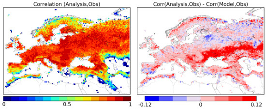
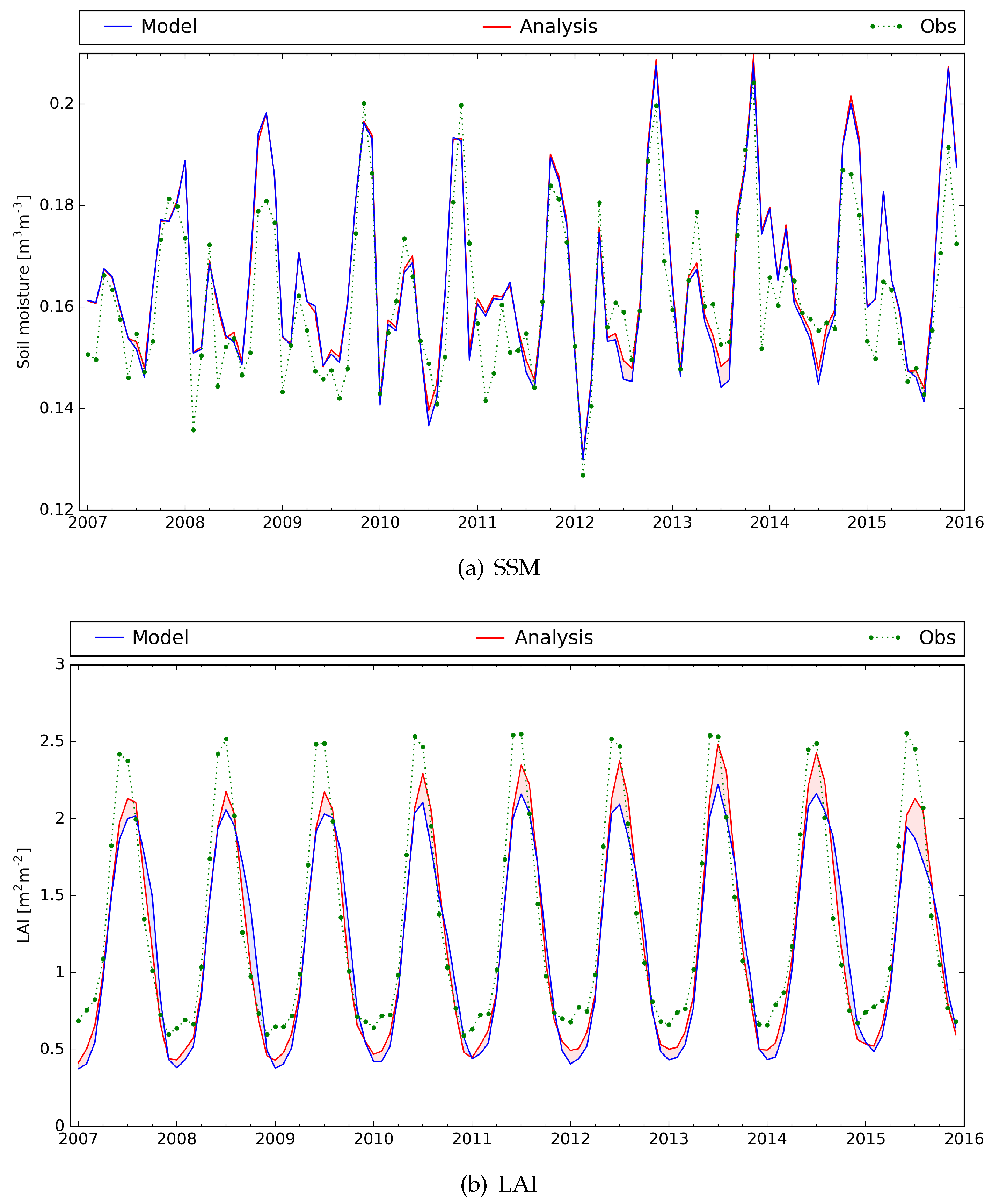
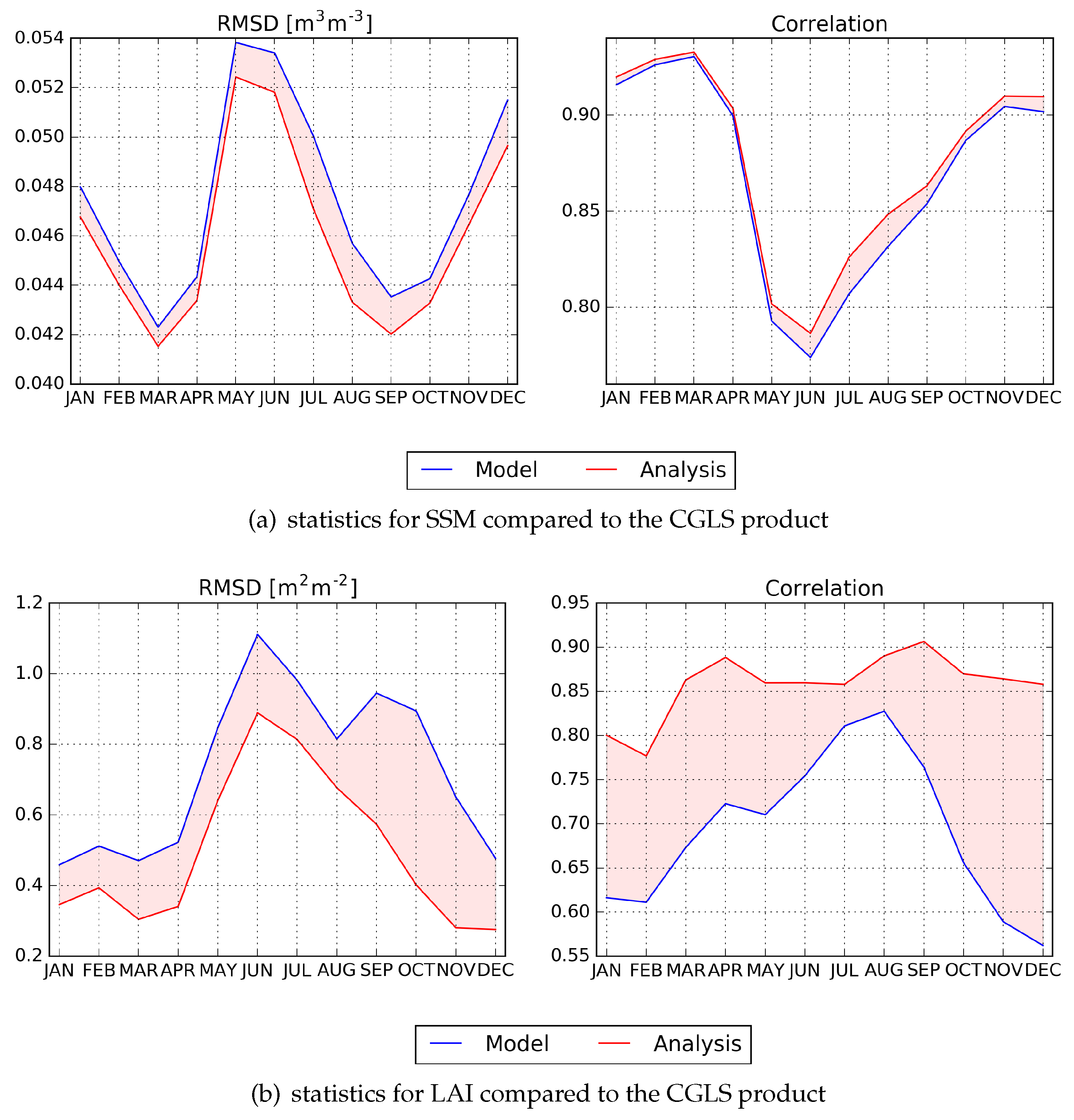
3.1. Impact of the Assimilation on SSM and LAI

In the assimilation process, the available observations were merged with the model simulations, weighted with their errors, as defined in [12,14], to compute an analysis taking into account all this information. It was expected that the analysis would end closer to the observations.
Figure 2 shows the monthly average open-loop simulations, analysis and observations of SSM and LAI over the Euro-Mediterranean area. The SSM analysis was very close to the open-loop since the SSM observations were rescaled before being assimilated. Open-loop and analysis scores for the whole time period and over each pixel were similar, as described in Table 1. These scores were computed using pooled pixel data during one month, so they included both spatial and temporal components.
The largest impacts of the assimilation process can be seen on the LAI variable. Figure 2 shows the LAI simulations and observations at the monthly scale. In summer and winter times, the open-loop simulations tended to underestimate LAI (compared to LAI observations), and the analysis simulations were closer to the observations after the assimilation. The statistics from Table 1 indicate a lower RMSD (−28%) and a better correlation R (+14%).
Figure 3 shows seasonal scores for each month of all years from 2007–2015 (RMSD and R). They were computed using all the pixels and dates available for each considered month. These statistics show an improvement for both SSM and LAI analyzed variables for all the months of the year. For SSM, the RMSD was always reduced, with analysis values ranging from about 0.042 m 3 ·m 3 in March and September to 0.054 m 3 ·m 3 in May and December. Correlation was slightly improved in winter and spring and more markedly improved in summer and during the autumn, with analysis values ranging from 0.77–0.94. Because of the seasonal rescaling of SSM, the seasonality in the statistics cannot be improved. Regarding LAI, both RMSD and R scores were improved during the year with analysis RMSD and R values ranging from 0.3–0.9 m 2 ·m 2 and from 0.77–0.91, respectively. The analyzed LAI was closer to the observations than the open-loop simulation throughout the year, in particular during the senescence phase where RMSD dropped from around 0.9 m 2 ·m 2 (open-loop) to around 0.4–0.6 m 2 ·m 2 (analysis) in September and October. A seasonality in the scores can clearly be seen with a larger open-loop SSM RMSD in summer and winter associated with a lower correlation in summer and larger open-loop LAI RMSD values in summer associated with a slightly better correlation in summer. After assimilation, the seasonality in the LAI correlation was smoothed out with R values between 0.78 and 0.90.

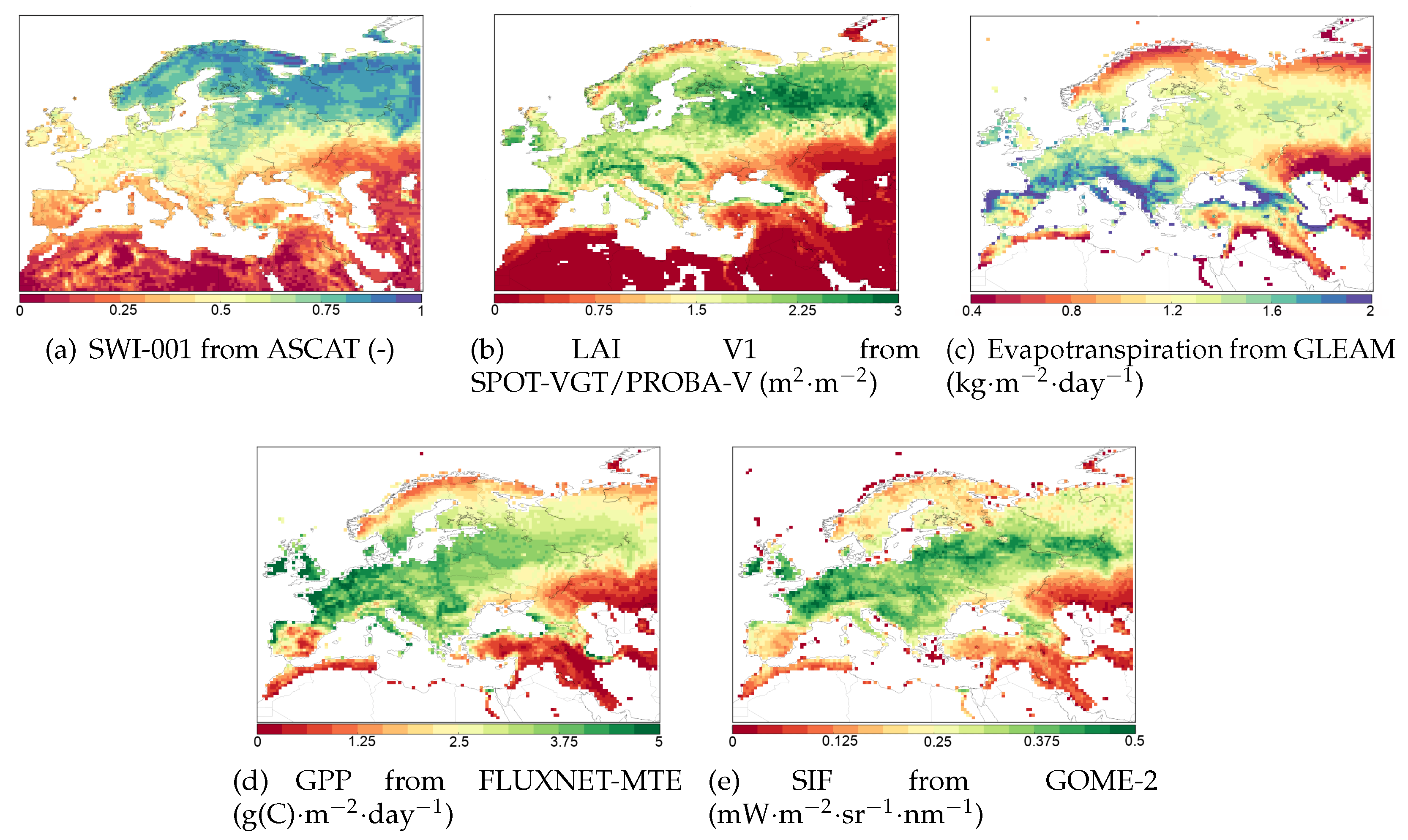
3.2. Evaluation Using Satellite-Derived Vegetation Products

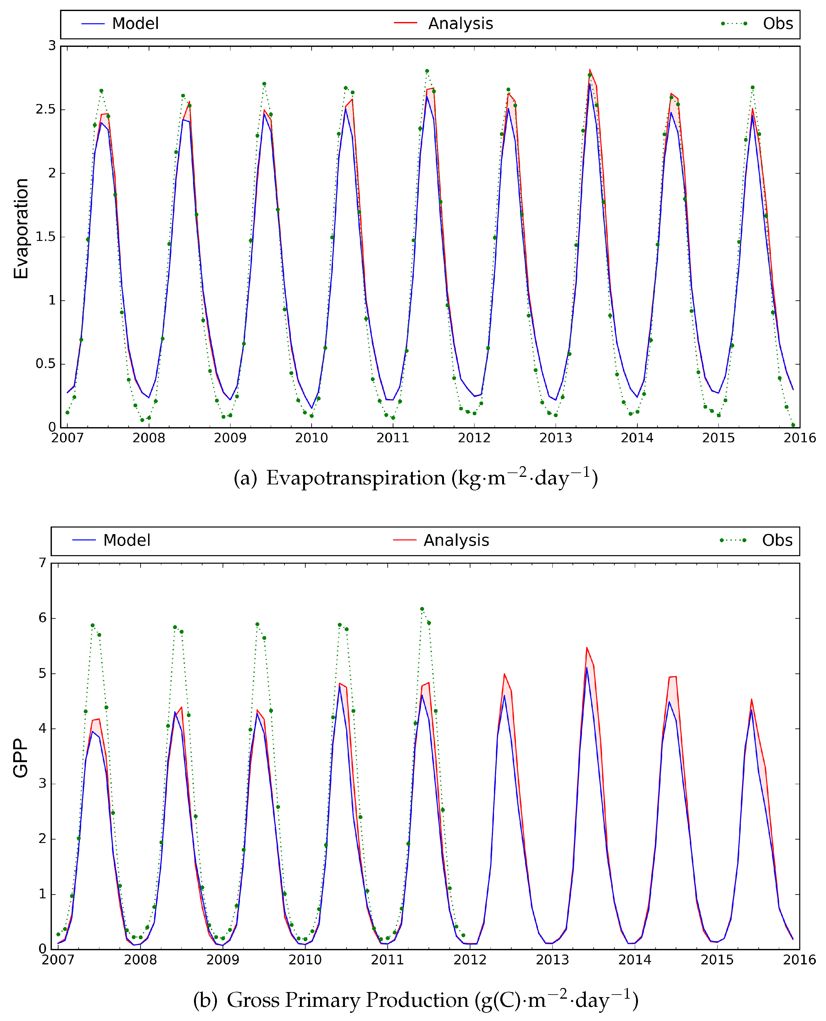
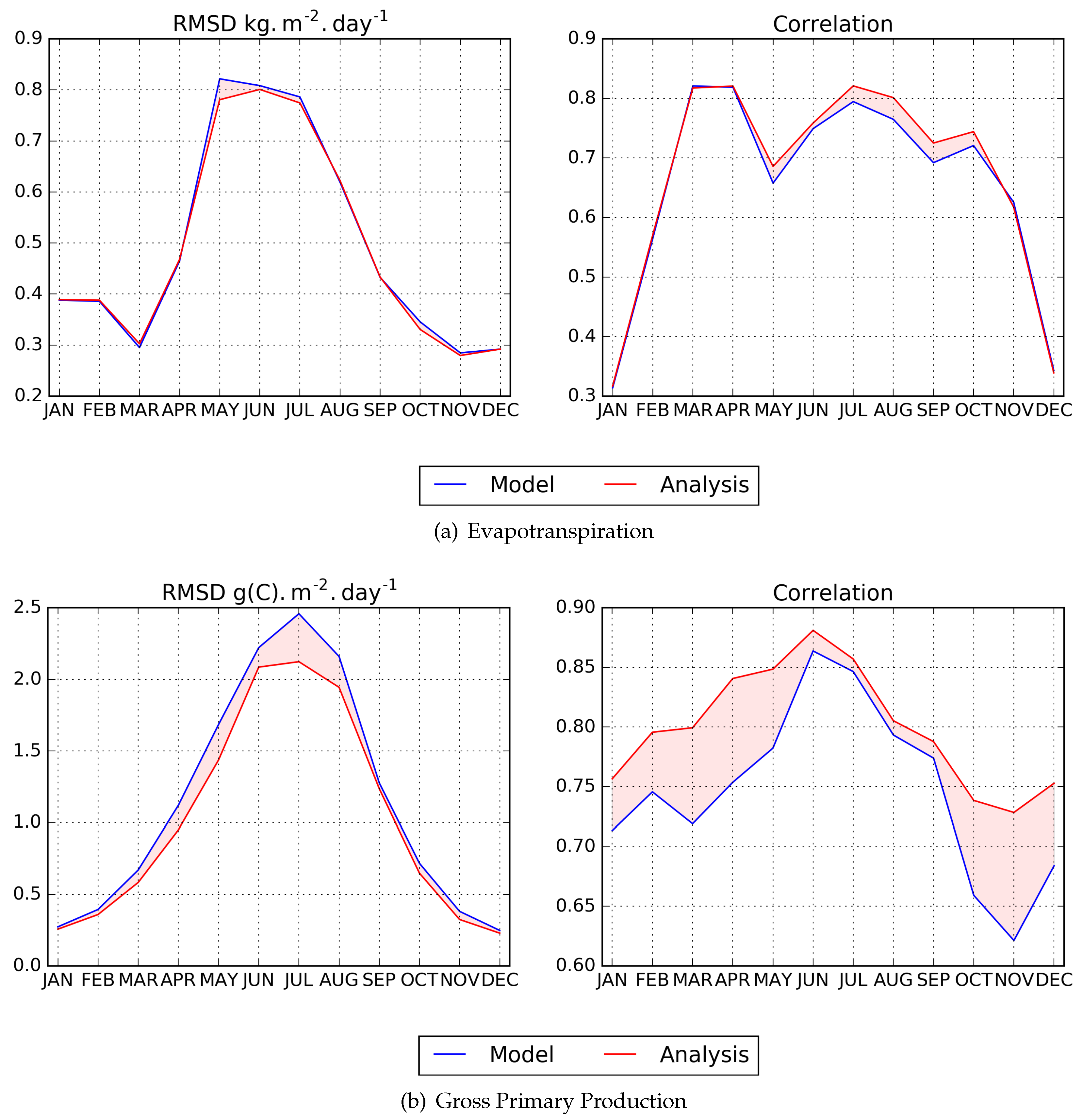
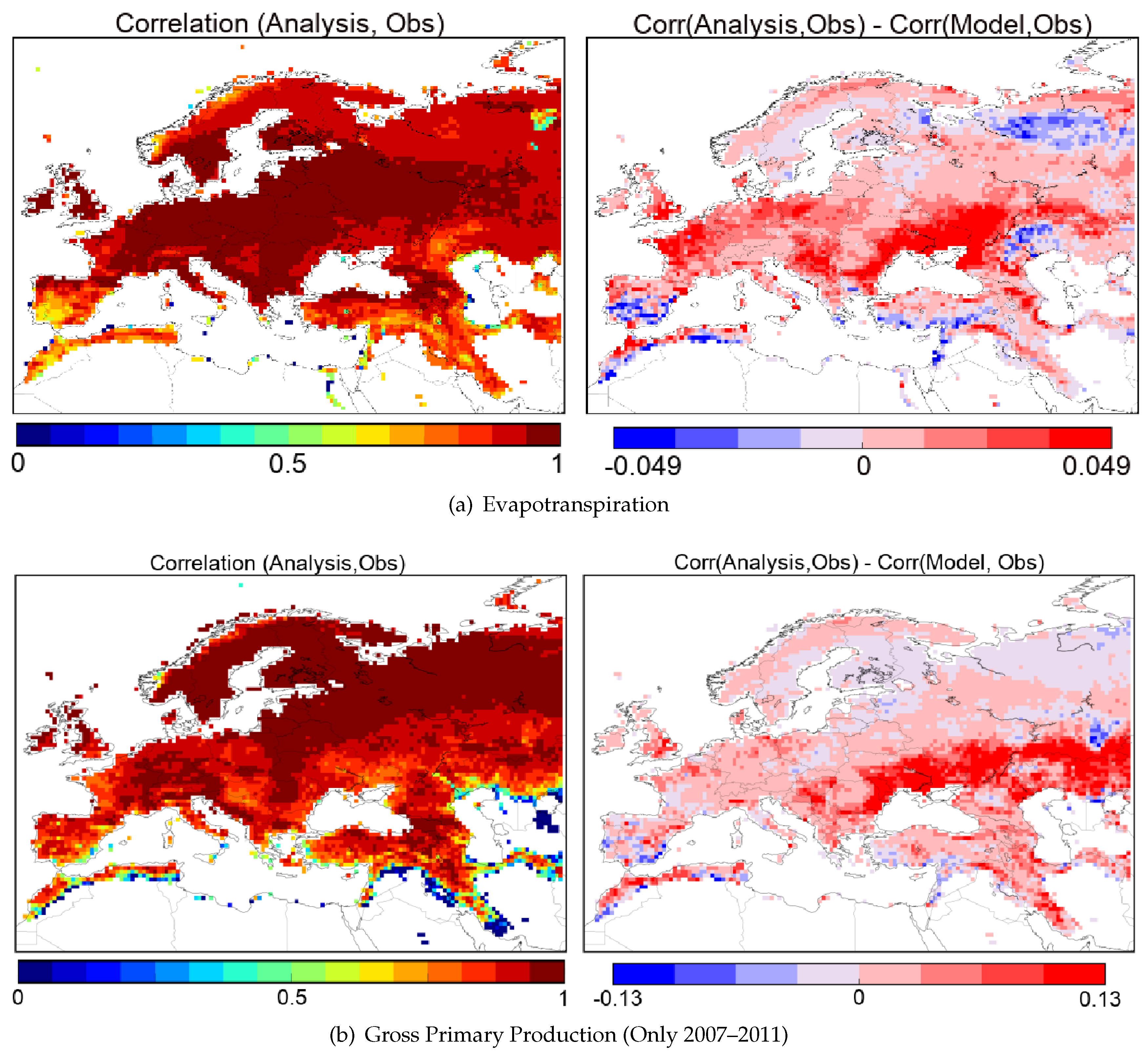
3.2.1. Evapotranspiration and GPP

The consistency of the analysis with the evapotranspiration product from the GLEAM product and the GPP product from the FLUXNET-MTE dataset is evaluated in this section. Since these products are only available at the monthly scale, they were compared to monthly averaged analyzed simulations. The GPP product from the FLUXNET-MTE dataset is only available until 2011, so only the years 2007–2011 are considered in the statistics below.
Figure 4 shows monthly mean time series of evapotranspiration and GPP over the Euro-Mediterranean area of the open-loop and analysis simulations and of the products. The dynamics of the simulated evapotranspiration variable was in line with GLEAM with a slight overestimation in winter and underestimation in summer. The impact of the assimilation was generally small, but is more noticeable during the summer season. The analyzed values were closer to the observations in the summer time. This was confirmed by the seasonal statistics shown in Figure 5, where they tend to be slightly better for the analysis during summer with lower RMSD values and higher correlation scores. Statistics for the whole time period (Table 1) showed that the assimilation of SSM and LAI products slightly improved the consistency of the model with GLEAM.
Compared to the LDAS analyzed evapotranspiration, the GLEAM product had an RMSD varying from 0.3 kg·m 2 ·day 1 in winter to 0.8 kg·m 2 ·day 1 between May and July. The highest RMSD values mainly occurred over forested areas (not shown).
Regarding the GPP variable, the simulated dynamics was consistent with FLUXNET-MTE, but the analyzed monthly GPP exceeded 5 g(C)·m 2 ·day 1 only once (in 2013), while FLUXNET-MTE seemed to exceed this value for all the years. The assimilation only slightly reduced the mean bias between the simulations and FLUXNET-MTE. However, Figure 5 shows that the assimilation markedly reduced RMSD in summer. The assimilation also significantly improved the correlation scores during the other seasons. The statistics were also slightly improved when looking at the whole time period (Table 1) with a decrease of 10% in the bias and in the Standard Deviation of Differences (SDD) values.
Compared to the LDAS analysis, the FLUXNET-MTE GPP product had a RMSD varying from 0.2 g(C)·m 2 ·day 1 in winter to 2 g(C)·m 2 ·day 1 between June and August. The highest RMSD values mainly occurred over areas covered by crops (not shown).
In Figure 6, temporal correlation maps are presented, representative of the time evolution of the variable itself at a specific location. This figure shows the spatial distribution of the correlation for the whole available period (2007–2015 for the evapotranspiration, 2007–2011 for GPP) between the analysis and the observations. The model open-loop simulations already gave very good results in terms of correlation with 65% of the points with a correlation greater than 0.90 for the evapotranspiration and 55% for GPP (not shown). After the joint assimilation of SSM and LAI, 70% and 64% of the points had a correlation higher than 0.90 respectively. As shown on the correlation difference map (right column of Figure 6), these improvements were mainly located on the northern part of the Black Sea and of the Caspian Sea, which are regions mainly covered by crops and grasslands. Some improvements in Western Europe were also visible for the evapotranspiration variable, which is also a region mainly covered by crops and grasslands. Blue areas indicate a degradation of the the correlation after the assimilation at northern latitudes over boreal forests and grasslands. It showed an inconsistency between the assimilated satellite products and the GLEAM evapotranspiration and FLUXNET-MTE GPP products in these regions. Further investigations are needed to explain this inconsistency.

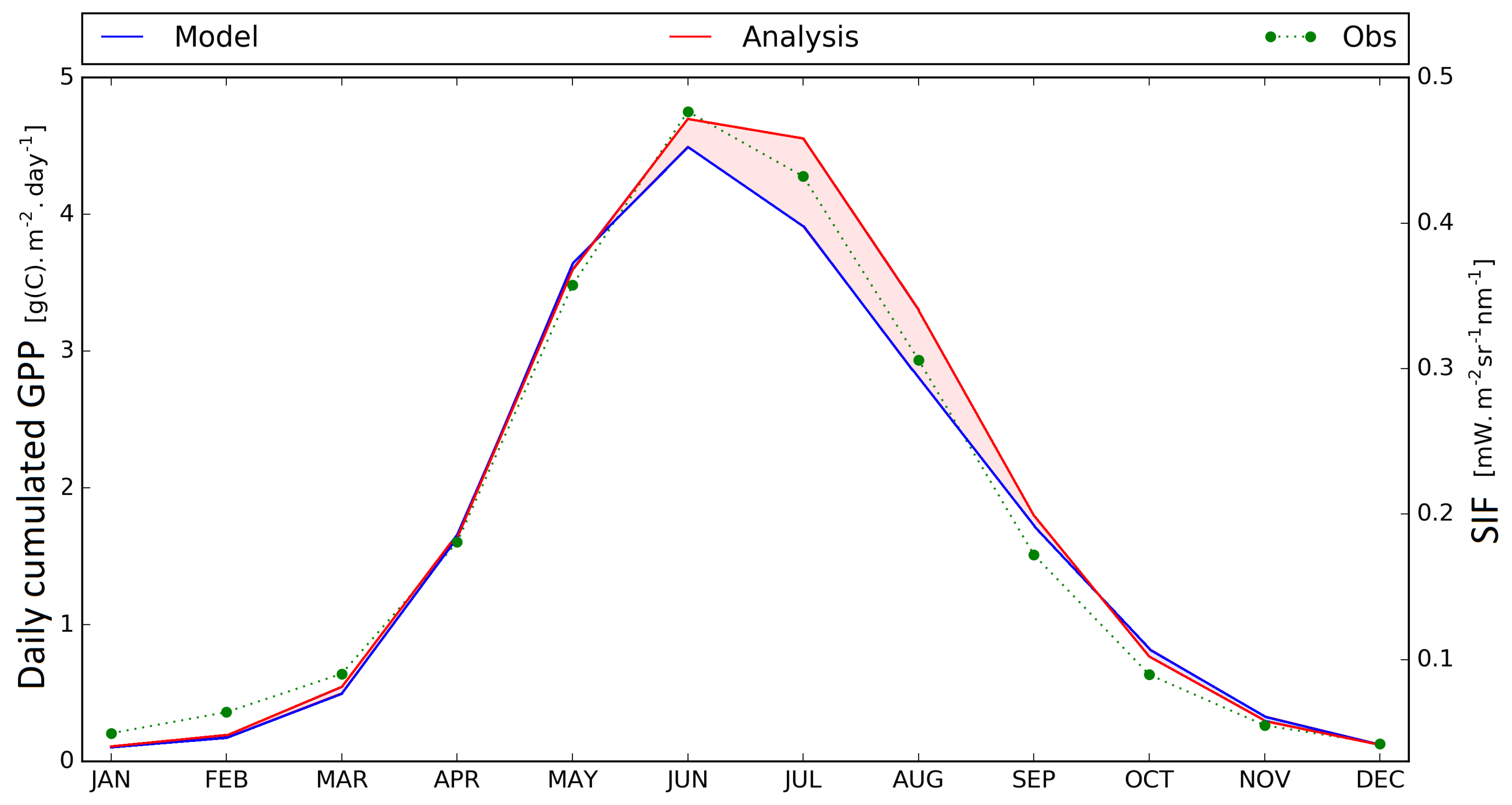
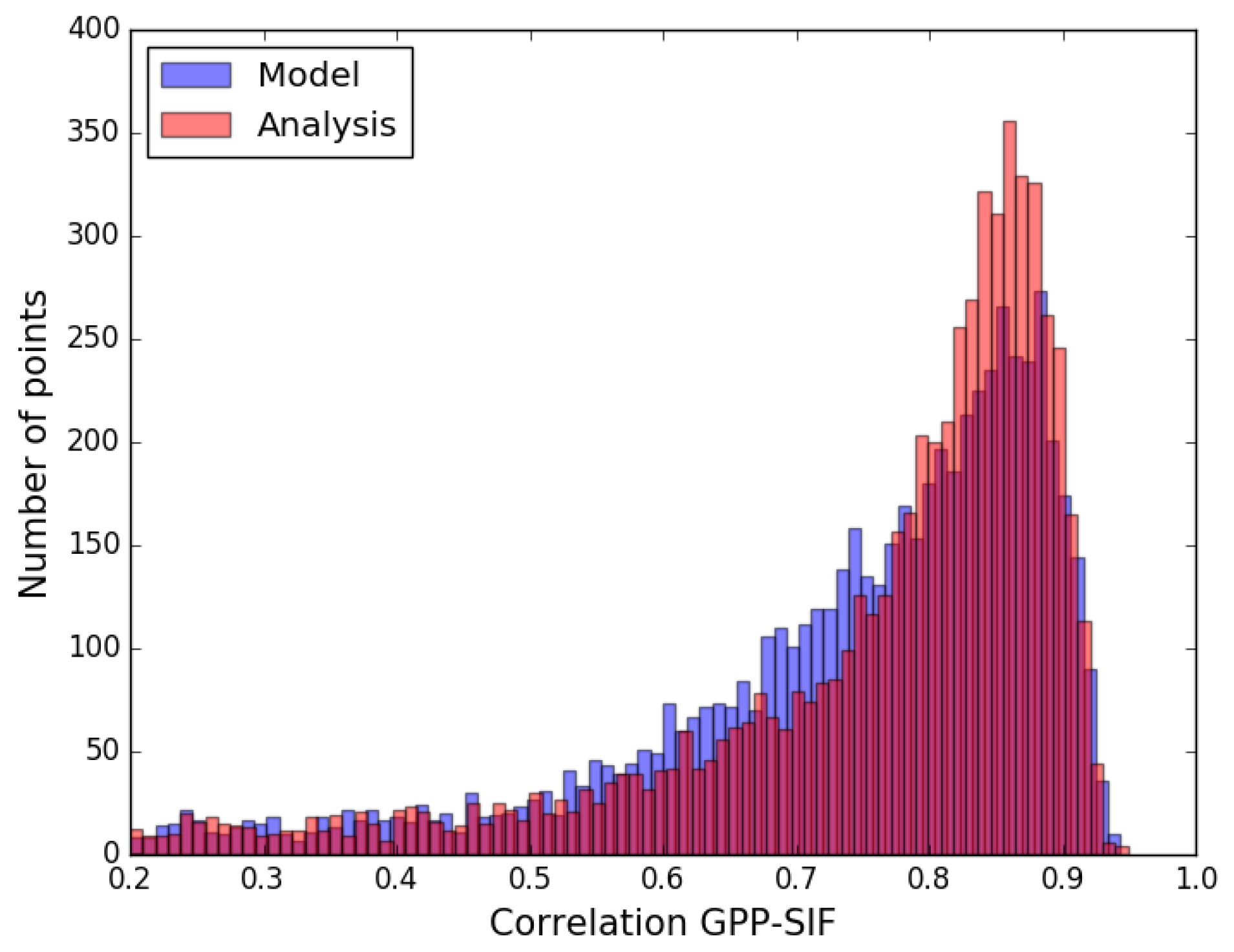
3.2.2. Sun-Induced Fluorescence

The modeled GPP values are expressed in g(C)·m 2 ·day 1 , whereas SIF is an energy flux emitted by the vegetation in units of mW·m 2 ·sr 1 ·nm 1 . Thus, GPP and SIF cannot be directly compared as they do not represent the same physical quantities. However, their time dynamics and their spatial distributions can be investigated. Figure 7 shows seasonal monthly time series of the modeled GPP (open-loop and analysis) with almost no photosynthesis activity during winter and a peak in the summer time. The SIF observations followed the same time evolution with very low values in winter and higher values in summer. Even if these two quantities are not quantitatively comparable, they followed the same evolution throughout the year.
Figure 8 represents the time correlation between the GPP analysis and the SIF products. The histogram of these correlation values in Figure 9 shows that the assimilation enhanced the consistency between the simulated GPP and SIF products, with more R values larger than 0.8 and fewer R values smaller than 0.8. These improvements were particularly large in cropland areas in Central Europe, the Ukraine and southern Russia, close to the Black Sea and the Caspian Sea. These areas coincide with those in Figure 6 presenting better model R values with GPP. This shows that the joint assimilation of the SSM and LAI products had a positive impact on other vegetation variables.
As already mentioned in previous studies, such as [24,59] or [60], the relationship between GPP and SIF can vary from one vegetation type to another. For this reason, the SIF-GPP relationship was investigated for each of the four main vegetation types covering the Euro-Mediterranean area. Only pixels with at least 50% of their surface covered by one of these vegetation types were considered. Figure 10 shows the selected pixels: 395 pixels of deciduous forest, 1088 pixels of coniferous forest, 372 pixels of C3 crops and 469 pixels of grassland. Whenever the couple of an observation and simulation is available, a direct comparison can be done as indicated in Figure 10 for the four vegetation types.
Based on these spatial averages, a linear regression was drawn for each vegetation type indicated by the purple lines. The corresponding slope, intercept, correlation coefficient and standard deviation can be found in Table 2. The slope values of the linear regression were different from those found by [24] (last three columns in Table 2) using another GPP model: MPI-BGC (Max Planck Institute-BioGeoChemical, [61,62]). The MPI-BGC GPP product relies on satellite-based estimates of FAPAR and is produced by upscaling in situ measurements of carbon dioxide, water and energy fluxes at the global scale. However, the relative order of the slope values for the different vegetation types is about the same. The largest slope was found for coniferous forests, denoting larger sensitivity of GPP to SIF for this vegetation type. These contrasting slope values indicate that the relationship between GPP and SIF depended on the vegetation type, which is in line with what was already found in [24] even using a different model.

4. Discussion

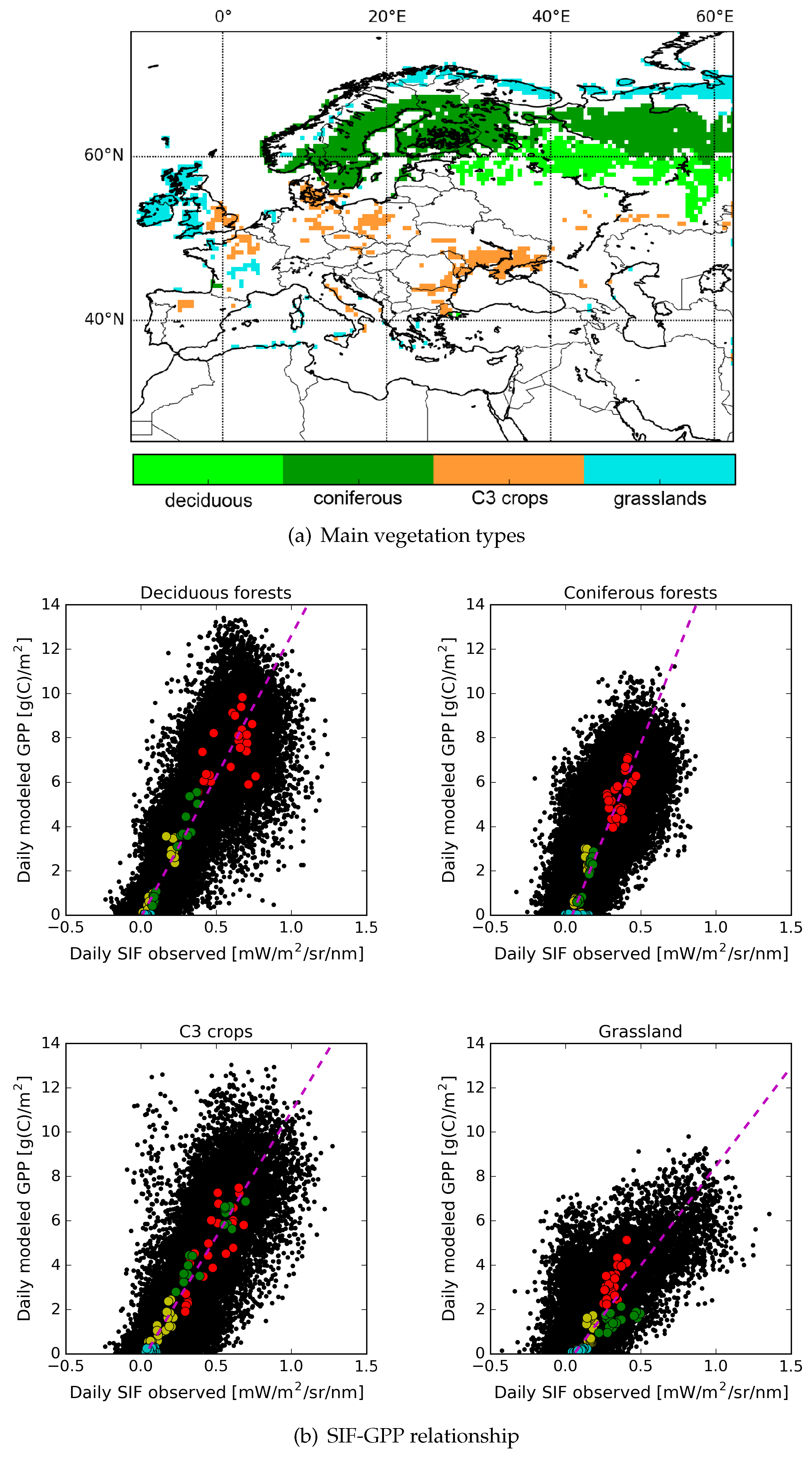
4.1. Investigating the SIF-GPP Relationship

In ISBA, the fluorescence is not simulated directly, but the photosynthesis activity is simulated through the calculation of the GPP, which is driven by plant growth and mortality in the model. Sun, Y. et al. [28] demonstrated that SIF and GPP were driven by the same environmental and biological factors and found that SIF observations from OCO-2 and GPP products from FLUXCOM were highly consistent in time and space. Their study was realized over various types of vegetation near Chicago, Illinois, U.S. At a much larger scale, the results of this study were consistent with [28], as the observed SIF from GOME-2 and the simulated GPP also showed a high correspondence in both time and space. This indicates that the SIF observations could be used as a relevant and independent source of validation for GPP model simulations.
The SCOPEmodel [63] allows the simulations of both SIF and GPP, but according to [64], who used SCOPE within a carbon cycle data assimilation system, SIF and GPP are not sensitive to the same physical parameters (the chlorophyll content and the maximum carboxylation rate, respectively). In this context, it was concluded that the assimilation of SIF observations cannot improve GPP simulations. By simplifying the SCOPE model and by computing the SIF from the GPP directly, [65] showed the potential of SIF to improve photosynthesis simulations. The results of this study showed a very good consistency between SIF and GPP, and the SIF-GPP relationship should be further investigated towards the construction of an observation operator in order to be able to assimilate SIF observations.
Unlike the study of [28], but in line with the studies of [24,59] or [60], the relationship between SIF and GPP was found to be dependent on the vegetation type. When all the pixels were used together to investigate the SIF-GPP relationship, no significant correlation could be found.
The ISBA model was also parameterized differently depending on the vegetation type, which could influence the SIF-GPP relationship in turn. Furthermore, the SIF products and the GPP simulations were at a low resolution (0.5 ), which might be too coarse to rule out any heterogeneity within the considered pixels. Moreover, the GOME-2 instrument footprint was 80 × 40 km, then rescaled on a 0.5 grid, so there might have also been some noise introduced by the rescaling process. It was however expected that this would have a small impact on the SIF-GPP relationship.
The Fluorescence EXplorer mission (FLEX, [66]) was selected by the European Space Agency as the eight Earth Explorer mission scheduled for launch in 2022. FLEX is specifically designed for the monitoring of the vegetation fluorescence with an imaging spectrometer covering the spectral range from 500–780 nm. The swath width will be 150 km, and the spatial resolution of the SIF product will be 300 m, allowing further and more precise studies on the SIF-GPP relationship.

4.2. Can SSM and LAI Assimilation Be Improved?

In this study, a single LAI value was assimilated over the whole model grid cell. This means that a single value was used for all the vegetation types present within the considered grid cell. As presented in [12], the Jacobians were calculated individually for each vegetation type, which made the Kalman gain and the increments depend on the vegetation type. Instead of using only one observation of LAI per pixel (especially when the model resolution is 0.5 and the one of the observations is a few hundred meters), the possibility of assimilating different values of LAI for each patch is under investigation. Based on a Kalman filtering technique developed by [67], CGLS LAI data have been disaggregated so that LAI values can be assimilated independently over each individual patch. This has a major impact on the analyzed LAI, but also on the other vegetation variables such as the evapotranspiration and GPP [68].
The assimilation of CGLS SSM (original SWI rescaled in the model dynamic range) presents some caveats, and these data depend on the exponential filter used on multiple observations from the ASCAT radar (backscatter coefficients) at C-band, or 5.3 GHz. In order to be able to assimilate SWI products into the model, a seasonal CDF matching is performed, which projects the observation values into the model space. This process reduces the impact of the SSM assimilation on the analyzed simulations. In order to improve LDAS-Monde analysis, building an observation operator for backscatter coefficients could be a way to overcome the use of the SWI product and directly assimilate the observed backscatter coefficients. Moreover, C-band observations also contain information on vegetation biomass. By building this forward operator, it would be thus possible to consider all the information contained in these observations. SSM products can also be derived from passive microwave satellite observations. In the same way as for the observed backscatter coefficients, building an operator for brightness temperatures (energy that is naturally emitted by the surface of the Earth and dependent on the soil moisture at L-band, or 1.4 GHz) is needed to take full advantage of the available observations.

5. Conclusions

This study investigates the joint assimilation of satellite-derived soil moisture and vegetation observations to yield improved estimates of hydrological and vegetation fields, as well as water and carbon fluxes at the land surface level. SSM and LAI products were assimilated in the CO 2 responsive version of the ISBA land surface model from 2007–2015 over the Euro-Mediterranean area. This joint assimilation in ISBA resulted in improvements in the representation of the vegetation processes.
Independent observations were used to quantify improvements in the simulated water and carbon fluxes, as well as in the modeled vegetation dynamics: LAI from Copernicus Global Land Service, evapotranspiration from the GLEAM dataset, GPP from the FLUXNET-MTE dataset and fluorescence from GOME-2 observations. GPP and evapotranspiration products present a similar temporal evolution with less accuracy during the winter season, but with higher correlation scores. The evapotranspiration product is less accurate over forested areas, whereas the GPP product tends to be less accurate over crop-covered areas.
Fluorescence cannot be directly evaluated using LDAS-Monde, since it is not simulated by the ISBA model, but it is a very good proxy to the photosynthesis process represented by the GPP. Fluorescence observations were compared to the LDAS-Monde-analyzed GPP in the model. This is the first time that fluorescence has been evaluated within the LDAS-Monde framework, and it shows a very good correlation with GPP in the condition that the evaluation is performed independently for each individual vegetation type. At 0.5 resolution, only pixels covered by at least 50% of their surface by one single vegetation type were considered, and a strong and linear relationship has been identified for deciduous forests, coniferous forests, C3 crops and grassland, which could be the translation of a different behavior in the photosynthesis process depending on the vegetation type. This also suggests that LDAS-Monde analysis can be used to study the possible relationship between the fluorescence and the GPP at the continental scale. This constitutes the first step to building an observation operator to assimilate fluorescence observations in view of the preparation of the future satellite mission FLEX, which is scheduled to be launched in 2022.
With more and more available satellite observations, the perspective of assimilating new products such as the surface albedo, radar backscatter coefficients or passive brightness temperatures looks extremely promising and will improve even more the LDAS-Monde analyses and our understanding of the various vegetation processes.

Author Contributions

D.J.L and J.-C.C conceived of and designed the experiments. D.J.L performed the experiments. All the authors analyzed the results. D.J.L wrote the paper.

Funding

The work of Delphine Leroux and Simon Munier was supported by the European Union Seventh Framework Programme (FP7/2007-2013) under Grant Agreement No. 603608, “Global Earth Observation for integrated water resource assessment” (eartH2Observe).

Acknowledgments

The authors acknowledge the Copernicus Global Land service for providing the satellite-derived LAI and soil moisture products.

Conflicts of Interest

The authors declare no conflict of interest.

Abbreviations

The following abbreviations are used in this manuscript:
LDASLand Data Assimilation System
SSMSurface Soil Moisture
LAILeaf Area Index
ISBAInteractions between Soil, Biosphere and Atmosphere
GLEAMGlobal Land surface Evaporation: the Amsterdam Methodology
FLUXNET-MTEFlux Network-Multi-Tree Ensemble
TERTerrestrial Ecosystem Respiration
GOMEGlobal Ozone Monitoring Experiment
LSMLand Surface Model
SURFEXSurface Externalisée
SIFSun-Induced chlorophyll Fluorescence
GOSATGreenhouse gas Observing Satellite
GPPGross Primary Productivity
GCOSGlobal Climate Observing System
CGLSCopernicus Global Land Service
SWISoil Water Index
EUMETSATEuropean Meteorological Satellite
JSBACHJena Scheme of Atmosphere Biosphere Coupling in Hamburg
RMSDRoot Mean Square Deviation
RCorrelation
STDSTandard Deviation
SDDStandard Deviation of Differences
FLEXFluorescence Explorer mission

References

  1. Noilhan, J.; Mahfouf, J.-F. The ISBA land surface parameterisation scheme. Glob. Planet. Chang. 1996, 13, 145–159. [Google Scholar] [CrossRef]
  2. Calvet, J.-C.; Noilhan, J.; Roujean, J.-L.; Bessemoulin, P.; Cabelguenne, M.; Olioso, A.; Wigneron, J.-P. An interactive vegetation SVAT model tested against data from six contrasting sites. Agric. For. Meteorol. 1998, 92, 73–95. [Google Scholar] [CrossRef]
  3. Gibelin, A.-L.; Calvet, J.-C.; Roujean, J.-L.; Jarlan, L.; Los, S.O. Ability of the land surface model ISBA-A-gs to simulate leaf area index at the global scale: comparison with satellite products. J. Geophys. Res. 2006, 111, D18102. [Google Scholar] [CrossRef]
  4. Houghton, J.; Ding, Y.; Griggs, D.; Noguer, M.; van der Linden, P.; Dai, X.; Maskell, K.; Johnson, C. (Eds.) Climate Change 2001: The Scientific Basis. Contribution of Working Group I to the Third Assessment Report of the Intergovernmental Panel on Climate Change; Cambridge University Press: New York, NY, USA, 2001. [Google Scholar]
  5. Reichle, R.; Walker, J.; Koster, R.; Houser, P. Extended vs. Ensemble Kalman Filtering for Land Data Assimilation. J. Hydrometeorol. 2002, 3, 728–740. [Google Scholar] [CrossRef]
  6. Draper, C.; Mahfouf, J.-F.; Calvet, J.-C.; Martin, E.; Wagner, W. Assimilation of ASCAT near-surface soil moisture into the SIM hydrological model over France. Hydrol. Earth Syst. Sci. 2011, 15, 3829–3841. [Google Scholar] [CrossRef] [Green Version]
  7. Draper, C.; Reichle, R.H.; De Lannoy, G.J.M.; Liu, Q. Assimilation of passive and active microwave soil moisture retrievals. Geophys. Res. Lett. 2012, 39, L04401. [Google Scholar] [CrossRef]
  8. Dharssi, I.; Bovis, K.J.; Macpherson, B.; Jones, C. Operational assimilation of ASCAT surface soil wetness at the Met Office. Hydrol. Earth Syst. Sci. 2011, 15, 2729–2746. [Google Scholar] [CrossRef] [Green Version]
  9. Barbu, A.L.; Calvet, J.-C.; Mahfouf, J.-F.; Albergel, C.; Lafont, S. Assimilation of Soil Wetness Index and Leaf Area Index into the ISBA-A-gs land surface model: Grassland case study. Biogeosciences 2011, 8, 1971–1986. [Google Scholar] [CrossRef] [Green Version]
  10. De Rosnay, P.; Drusch, M.; Vasiljevic, D.; Balsamo, G.; Albergel, C.; Isaksen, L. A simplified Extended Kalman Filter for the global operational soil moisture analysis at ECMWF. Q. J. R. Meteorol. Soc. 2013, 139, 1199–1213. [Google Scholar] [CrossRef]
  11. De Rosnay, P.; Balsamo, G.; Albergel, C.; Munoz-Sabater, J.; Isaksen, L. Initialisation of land surface variables for Numerical Weather Prediction. Surv. Geophys. 2014, 35, 607–621. [Google Scholar] [CrossRef]
  12. Barbu, A.L.; Calvet, J.-C.; Mahfouf, J.-F.; Lafont, S. Integrating ASCAT surface soil moisture and GEOV1 leaf area index into the SURFEX modelling platform: A land data assimilation application over France. Hydrol. Earth Syst. Sci. 2014, 18, 173–192. [Google Scholar] [CrossRef] [Green Version]
  13. Boussetta, S.; Balsamo, G.; Dutra, E.; Beljaars, A.; Albergel, C. Assimilation of surface albedo and vegetation states from satellite observations and their impact on numerical weather prediction. Remote Sens. Environ. 2015, 163, 111–126. [Google Scholar] [CrossRef] [Green Version]
  14. Fairbairn, D.; Barbu, A.L.; Napoly, A.; Albergel, C.; Mahfouf, J.-F.; Calvet, J.-C. The effect of satellite-derived surface soil moisture and leaf area index land data assimilation on streamflow simulations over France. Hydrol. Earth Syst. Sci. 2017, 21, 2015–2033. [Google Scholar] [CrossRef]
  15. Albergel, C.; Munier, S.; Leroux, D.J.; Dewaele, H.; Fairbairn, D.; Barbu, A.L.; Gelati, E.; Dorigo, W.; Faroux, S.; Meurey, C.; et al. Sequential assimilation of satellite-derived vegetation and soil moisture products using SURFEX v8.0: LDAS-Monde assessment over the Euro-Mediterranean area. Geosci. Model Dev. 2017, 10, 3889–3912. [Google Scholar] [CrossRef]
  16. Wang, L.; D’Odorico, P.; Evans, J.P.; Eldridge, D.; McCabe, M.F.; Caylor, K.K.; King, E.G. Dryland ecohydrology and climate change: Critical issues and technical advances. Hydrol. Earth Syst. Sci. 2012, 16, 2585–2603. [Google Scholar] [CrossRef] [Green Version]
  17. Kaminski, T.; Knorr, W.; Schurmann, G.; Scholze, M.; Rayner, P.J.; Zaehle, S.; Blessing, S.; Dorigo, W.; Gayler, V.; Giering, R.; et al. The BETHY/JSBACH Carbon Cycle Data Assimilation System: Experiences and challenges. J. Geophys. Res. Biogeosci. 2013, 118, 1414–1426. [Google Scholar] [CrossRef]
  18. Traore, A.K.; Ciais, P.; Vuichard, N.; Poulter, B.; Viovy, N.; Guimberteau, M.; Jung, M.; Myneni, R.; Fisher, J.B. Evaluation of the ORCHIDEE ecosystem model over Africa against 25 years of satellite-based water and carbon measurements. J. Geophys. Res. Biogeosci. 2014, 119, 2014JG002638. [Google Scholar] [CrossRef]
  19. Mohr, K.I.; Famiglietti, J.S.; Boone, A.; Starks, P.J. Modeling soil moisture and surface flux variability with an untuned land surface scheme: A case study from the Southern Great Plains 1997 Hydrology Experiment. J. Hydrometeorol. 2000, 1, 154–169. [Google Scholar] [CrossRef]
  20. Masson, V.; Le Moigne, P.; Martin, E.; Faroux, S.; Alias, A.; Alkama, R.; Belamari, S.; Barbu, A.; Boone, A.; Bouyssel, F.; et al. The SURFEXv7.2 land and ocean surface platform for coupled or offline simulation of earth surface variables and fluxes. Geosci. Model Dev. 2013, 6, 929–960. [Google Scholar] [CrossRef] [Green Version]
  21. Frankenberg, C.; Fisher, J.B.; Worden, J.; Badgley, G.; Saatchi, S.S.; Lee, J.-E.; Toon, G.C.; Butz, A.; Jung, M.; Kuze, A.; et al. New global observations of the terrestrial carbon cycle from GOSAT: Patterns of plant fluorescence with gross primary productivity. Geophys. Res. Lett. 2011, 38, L17706. [Google Scholar] [CrossRef]
  22. Frankenberg, C.; O’Dell, C.; Guanter, L.; McDuffie, J. Remote sensing of near-infrared chlorophyll fluorescence from space in scattering atmospheres: Implications for its retrieval and interferences with atmospheric CO2 retrievals. Atmos. Meas. Tech. 2012, 5, 2081–2094. [Google Scholar] [CrossRef]
  23. Joiner, J.; Yoshida, Y.; Vasilkov, A.P.; Yoshida, Y.; Corp, L.A.; Middleton, E.M. First observations of global and seasonal terrestrial chlorophyll fluorescence from space. Biogeosciences 2011, 8, 637–651. [Google Scholar] [CrossRef] [Green Version]
  24. Guanter, L.; Frankenberg, C.; Dudhia, A.; Lewis, P.E.; Gomez-Dans, J.; Kuze, A.; Suto, H.; Grainger, R.G. Retrieval and global assessment of terrestrial chlorophyll fluorescence from GOSAT space measurements. Remote Sens. Environ. 2012, 121, 236–251. [Google Scholar] [CrossRef]
  25. Joiner, J.; Yoshida, Y.; Vasilkov, A.P.; Middleton, E.M.; Campbell, P.K.E.; Yoshida, Y.; Kuze, A.; Corp, L.A. Filling-in of near-infrared solar lines by terrestrial fluorescence and other geophysical effects: simulations and space-based observations from SCIAMACHY and GOSAT. Atmos. Meas. Tech. 2012, 5, 809–829. [Google Scholar] [CrossRef]
  26. Joiner, J.; Guanter, L.; Lindstrot, R.; Voigt, M.; Vasilkov, A.P.; Middleton, E.M.; Huemmrich, K.F.; Yoshida, Y.; Frankenberg, C. Global monitoring of terrestrial chlorophyll fluorescence from moderate-spectral-resolution near-infrared satellite measurements: methodology, simulations, and application to GOME-2. Atmos. Meas. Tech. 2013, 6, 2803–2823. [Google Scholar] [CrossRef] [Green Version]
  27. Zhang, Y.; Xiao, X.; Jin, C.; Dong, J.; Zhou, S.; Wagle, P.; Joiner, J.; Guanter, L.; Zhang, Y.; Zhang, G.; et al. Consistency between sun-induced chlorophyll fluorescence and gross primary production of vegetation in North America. Remote Sens. Environ. 2016, 183, 154–169. [Google Scholar] [CrossRef] [Green Version]
  28. Sun, Y.; Frankenberg, C.; Wood, J.D.; Schimel, D.S.; Jung, M.; Guanter, L.; Drewry, D.T.; Verma, M.; Porcar-Castell, A.; Griffis, T.J.; et al. OCO-2 advances photosynthesis observation from space via solar-induced chlorophyll fluorescence. Science 2017, 358, 189. [Google Scholar] [CrossRef] [PubMed]
  29. Miralles, D.G.; Holmes, T.R.H.; de Jeu, R.A.M.; Gash, J.H.; Meesters, A.G.C.A.; Dolman, A.J. Global land-surface evaporation estimated from satellite-based observations. Hydrol. Earth Syst. Sci. 2011, 15, 453–469. [Google Scholar] [CrossRef] [Green Version]
  30. Jung, M.; Reichstein, M.; Bondeau, A. Towards global empirical upscaling of FLUXNET eddy covariance observations: validation of a model tree ensemble approach using a biosphere model. Biogeosciences 2009, 6, 2001–2013. [Google Scholar]
  31. Boone, A.; Calvet, J.-C.; Noilhan, J. Inclusion of a third soil layer in a land surface scheme using the force-restore method. J. Appl. Meteorol. 1999, 38, 1611–1630. [Google Scholar] [CrossRef]
  32. Calvet, J.-C.; Soussana, J.-F. Modelling CO2-enrichment effects using an interactive vegetation SVAT scheme. Agric. For. Meteorol. 2001, 108, 129–152. [Google Scholar] [CrossRef]
  33. Calvet, J.-C. Investigating soil and atmospheric plant water stress using physiological and micrometeorological data. Agric. For. Meteorol. 2000, 103, 229–247. [Google Scholar] [CrossRef]
  34. Calvet, J.-C.; Rivalland, V.; Picon-Cochard, C.; Guehl, J.-M. Modelling forest transmiration and CO2 fluxes-response to soil moisture stress. Agric. For. Meteorol. 2004, 124, 143–156. [Google Scholar] [CrossRef]
  35. Jacobs, C.M.J.; van den Hurk, B.J.J.M.; de Bruin, H.A.R. Stomatal behaviour and photosynthetic rate of unstressed grapevines in semi-arid conditions. Agric. For. Meteorol. 1996, 80, 111–134. [Google Scholar] [CrossRef]
  36. Lafont, S.; Zhao, Y.; Calvet, J.-C.; Peylin, P.; Ciais, P.; Maignan, F.; Weiss, M. Modelling LAI, surface water and carbon fluxes at high-resolution over France: Comparison of ISBA-A-gs and ORCHIDEE. Biogeosciences 2012, 9, 439–456. [Google Scholar] [CrossRef]
  37. Szczypta, C.; Calvet, J.-C.; Maignan, F.; Dorigo, W.; Baret, F.; Ciais, P. Suitability of modelled and remotely sensed essential climate variables for monitoring Euro-Mediterranean droughts. Geosci. Model Dev. 2014, 7, 931–946. [Google Scholar] [CrossRef] [Green Version]
  38. Mahfouf, J.-F.; Bergaoui, K.; Draper, C.; Bouyssel, F.; Taillefer, F.; Taseva, L. A comparison of two off-line soil analysis schemes for assimilation of screen level observations. J. Geophys. Res. 2009, 114, D08105. [Google Scholar] [CrossRef]
  39. Albergel, C.; Calvet, J.-C.; Mahfouf, J.-F.; Rüdiger, C.; Barbu, A.L.; Lafont, S.; Roujean, J.-L.; Walker, J.P.; Crapeau, M.; Wigneron, J.-P. Monitoring of water and carbon fluxes using a land data assimilation system: A case study for southwestern France. Hydrol. Earth Syst. Sci. 2010, 14, 1109–1124. [Google Scholar] [CrossRef] [Green Version]
  40. Faroux, S.; Kaptue Tchuente, A.T.; Roujean, J.-L.; Masson, V.; Martin, E.; Le Moigne, P. ECOCLIMAP-II/ Europe: A twofold database of ecosystems and surface parameters at 1 km resolution based on satellite information for use in land surface, meteorological and climate models. Geosci. Model Dev. 2013, 6, 563–582. [Google Scholar] [CrossRef]
  41. Albergel, C.; Rüdiger, C.; Pellarin, T.; Calvet, J.-C.; Fritz, N.; Froissard, F.; Suquia, D.; Petitpa, A.; Piguet, B.; Martin, E. From near-surface to root-zone soil moisture using an exponential filter: An assessment of the method based on in-situ observations and model simulations. Hydrol. Earth Syst. Sci. 2008, 12, 1323–1337. [Google Scholar] [CrossRef]
  42. Wagner, W.; Lemoine, G.; Rott, H. A method for estimating soil moisture from ERS scatterometer and soil data. Remote Sens. Environ. 1999, 70, 191–207. [Google Scholar] [CrossRef]
  43. Bartalis, Z.; Wagner, W.; Naeimi, V.; Hasenauer, S.; Scipal, K.; Bonekamp, H.; Figa, J.; Anderson, C. Initial soil moisture retrievals from the METOP-A Advanced Scatterometer (ASCAT). Geophys. Res. Lett. 2007, 34, L20401. [Google Scholar] [CrossRef]
  44. Reichle, R.H.; Koster, D. Bias reduction in short records of satellite soil moisture. Geophys. Res. Lett. 2004, 31, L19501. [Google Scholar] [CrossRef]
  45. Drusch, M.; Wood, E.F.; Gao, H. Observations operators for the direct assimilation of TRMM microwave imager retrieved soil moisture. Geophys. Res. Lett. 2005, 32, L15403. [Google Scholar] [CrossRef]
  46. Scipal, K.; Drusch, M.; Wagner, W. Assimilation of a ERS scatterometer derived soil moisture index in the ECMWF numerical weather prediction system. Adv. Water Resour. 2008, 31, 1101–1112. [Google Scholar] [CrossRef]
  47. Baret, F.; Weiss, M.; Lacaze, R.; Camacho, F.; Makhmara, H.; Pacholcyzk, P.; Smets, B. GEOV1: LAI and FAPAR essential climate variables and FCOVER global time series capitalizing over existing products. Part1: Principles of development and production. Remote Sens. Environ. 2013, 137, 299–309. [Google Scholar] [CrossRef]
  48. Baret, F.; Hagolle, O.; Geiger, B.; Bicheron, P.; Miras, B.; Huc, M.; Berthelot, B.; Nino, F.; Weiss, M.; Samain, O.; et al. LAI, fAPAR and fCover CYCLOPES global products derived from VEGETATION. Part 1: Principles of the algorithm. Remote Sens. Environ. 2007, 110, 275–286. [Google Scholar] [CrossRef] [Green Version]
  49. Yang, W.; Shabanov, N.V.; Huang, D.; Wang, W.; Dickinson, R.E.; Nemani, R.R.; Knyazikhin, Y.; Myneni, R.B. Analysis of leaf area index products from combination of MODIS Terra and Aqua data. Remote Sens. Environ. 2006, 104, 297–312. [Google Scholar] [CrossRef]
  50. Martens, B.; Miralles, D.G.; Lievens, H.; van der Schalie, R.; de Jeu, R.A.M.; Fernandez-Prieto, D.; Beck, H.E.; Dorigo, W.A.; Verhoest, N.E.C. GLEAM v3: Satellite-based land evaporation and root-zone soil moisture. Geosci. Model Dev. 2017, 10, 1903–1925. [Google Scholar] [CrossRef]
  51. Baldocchi, D.T. Breathing of the terrestrial biosphere: Lessons learned from a global network of carbon dioxide flux measurement systems. Aust. J. Bot. 2008, 56, 1–26. [Google Scholar] [CrossRef]
  52. Reichstein, M.; Falge, E.; Baldocchi, D.; Papale, D.; Aubinet, M.; Berbigier, P.; Bernhofer, C.; Buchmann, N.; Gilmanov, T.; Granier, A.; et al. On the separation of net ecosystem exchange into assimilation and ecosystem respiration: review and improved algorithm. Glob. Chang. Biol. 2005, 11, 1424–1439. [Google Scholar] [CrossRef]
  53. Lasslop, G.; Reichstein, M.; Papale, D.; Richardson, A.D.; Arneth, A.; Barr, A.; Stoy, P.; Wohlfahrt, G. Separation of net ecosystem exchange into assimilation and respiration using a light response curve approach: Critical issues and global evaluation. Glob. Chang. Biol. 2010, 16, 187–208. [Google Scholar] [CrossRef]
  54. Munro, R.; Eisinger, M.; Anderson, C.; Callies, J.; Corpaccioli, E.; Lang, R.; Lefebvre, A.; Livschitz, Y.; Perez Albinana, A. GOME-2 on MetOp: From in-orbit verification to routine operations. In Proceedings of the EUMETSAT Meteorological Satellite Conference, Helsinki, Finland, 12–16 June 2006. [Google Scholar]
  55. Joiner, J.; Yoshida, Y.; Guanter, L.; Middleton, E.M. New methods for the retrieval of chlorophyll red fluorescence from hyperspectral satellite instruments: Simulations and application to GOME-2 and SCIAMACHY. Atmos. Meas. Tech. 2016, 9, 3939–3967. [Google Scholar] [CrossRef]
  56. Thum, T.; Zaehle, S.; Kohler, P.; Aalto, T.; Aurela, M.; Guanter, L.; Kolari, P.; Laurila, T.; Lohila, A.; Magnani, F.; et al. Modelling sun-induced fluorescence and photosynthesis with a land surface model at local and regional scales in northern Europe. Biogeosciences 2017, 14, 1969–1987. [Google Scholar] [CrossRef]
  57. Reick, C.H.; Raddatz, T.; Brovkin, V.; Gayler, V. Representation of natural and anthropogenic land cover change in MPI-ESM. J. Adv. Model. Earth Syst. 2013, 5, 459–482. [Google Scholar] [CrossRef] [Green Version]
  58. Dee, D.P.; Uppala, S.M.; Simmons, A.J.; Berrisford, P.; Poli, P.; Kobayashi, S.; Andrae, U.; Balmaseda, M.A.; Balsamo, G.; Bauer, P.; et al. The ERA-Interim reanalysis: Configuration and performance of the data assimilation system. Q. J. R. Meteorol. Soc. 2011, 137, 553–597. [Google Scholar] [CrossRef]
  59. Guanter, L.; Zhang, Y.; Jung, M.; Joiner, J.; Voigt, M.; Berry, J.A.; Frankenberg, C.; Huete, A.R.; Zarco-Tejada, P.; Lee, J.-E.; et al. Global and time-resolved monitoring of crop photosynthesis with chlorophyll fluorescence. Proc. Natl. Acad. Sci. USA 2014, 111, E1327–E1333. [Google Scholar] [CrossRef] [PubMed] [Green Version]
  60. Duveiller, G.; Cescatti, A. Spatially downscaling sun-induced chlorophyll fluorescence leads to an improved temporal correlation with gross primary productivity. Remote Sens. Environ. 2016, 182, 72–89. [Google Scholar] [CrossRef]
  61. Jung, M.; Reichstein, M.; Margolis, H.A.; Cescatti, A.; Richardson, A.D.; Altaf Arain, M.; Arneth, A.; Bernhofer, C.; Bonal, D.; Chen, J.; et al. Global patterns of land-atmosphere fluxes of carbon dioxide, latent heat, and sensible heat from eddy covariance, satellite, and meteorological observations. J. Geophys. Res. Biogeosci. 2011, 116, G00J07. [Google Scholar] [CrossRef]
  62. Jung, M.; Reichstein, M.; Margolis, H.A.; Cescatti, A.; Richardson, A.D.; Altaf Arain, M.; Arneth, A.; Bernhofer, C.; Bonal, D.; Chen, J.; et al. Corrections to Global patterns of land-atmosphere fluxes of carbon dioxide, latent heat, and sensible heat from eddy covariance, satellite, and meteorological observations. J. Geophys. Res. Biogeosci. 2012, 117, G04011. [Google Scholar] [CrossRef]
  63. Van der Tol, C.; Verhoef, W.; Timmermans, J.; Verhoef, A.; Su, Z. An integrated model of soil-canopy spectral radiances, photosynthesis, fluorescence, temperature and energy balance. Biogeosciences 2009, 6, 3109–3129. [Google Scholar] [CrossRef] [Green Version]
  64. Koffi, E.Ñ.; Rayner, P.J.; Norton, A.J.; Frankenberg, C.; Scholze, M. Investigating the usefulness of satellite-derived fluorescence data in inferring gross primary productivity within the carbon cycle data assimilation system. Biogeosciences 2015, 12, 4067–4084. [Google Scholar] [CrossRef]
  65. Lee, J.-E.; Berry, J.A.; van der Tol, C.; Yang, X.; Guanter, L.; Damm, A.; Baker, I.; Frankenberg, C. Simulations of chlorophyll fluorescence incorporated into the Community Land Model version 4. Glob. Chang. Biol. 2015, 21, 3469–3477. [Google Scholar] [CrossRef] [PubMed] [Green Version]
  66. Drusch, M.; Moreno, J.; Del Bello, U.; Franco, R.; Goulas, Y.; Huth, A.; Kraft, S.; Middleton, E.M.; Miglietta, F.; Mohammed, G.; et al. The Fluorescence EXplorer Mission Concept—ESA’s Earth Explorer 8. IEEE Trans. Geosci. Remote Sens. 2017, 55, 1273–1284. [Google Scholar] [CrossRef]
  67. Carrer, D.; Meurey, C.; Ceamanos, X.; Roujean, J.-L.; Calvet, J.-C.; Liu, S. Dynamic mapping of snow-free vegetation and bare soil albedos at global 1 km scale from 10 year analysis of MODIS satellite products. Remote Sens. Environ. 2014, 140, 420–432. [Google Scholar] [CrossRef]
  68. Munier, S.; Carrer, D.; Planque, C.; Camacho, F.; Albergel, C.; Calvet, J.C. Satellite Leaf Area Index: Global scale analysis of the tendencies per vegetation type over the last 17 years. Remote Sens. 2018, 10, 424. [Google Scholar] [CrossRef]
Figure 1. Averaged satellite-derived products for the whole period from 2007–2015: (a) original Soil Water Index (SWI); (b) Leaf Area Index (LAI); (c) evapotranspiration; (d) Gross Primary Production (GPP) and (e) Sun-Induced Fluorescence (SIF).
Remotesensing 10 01199 g001
Figure 2. Monthly time series of the observations (green), open-loop (blue) and analysis (red) simulations from 2007–2015 averaged over the Euro-Mediterranean area for: (a) Surface Soil Moisture (SSM) and (b) Leaf Area Index (LAI).
Remotesensing 10 01199 g002
Figure 3. Monthly seasonal scores (RMSD and correlation R) of the open-loop (blue) and analysis (red) simulations from 2007–2015 averaged over the Euro-Mediterranean area compared to the observations of: (a) SSM and (b) LAI. Red shade indicates an improvement from the assimilation process with either a lower error or a higher correlation score.
Remotesensing 10 01199 g003
Figure 4. Monthly time series of the products (green), open-loop (blue) and analysis (red) simulations from 2007 to 2015 averaged over the Euro-Mediterranean area for: (a) evapotranspiration; (b) gross primary production (observations only until 2011).
Remotesensing 10 01199 g004
Figure 5. Monthly seasonal scores (RMSD and correlation) of the open-loop (blue) and analysis (red) simulations from 2007–2015 averaged over the Euro-Mediterranean area compared to the products of: (a) GLEAM Evapotranspiration (E) and (b) FLUXNET-MTE gross primary production (only 2007–2011). Red shade indicates an improvement from the assimilation process with either a lower error or a higher correlation score.
Remotesensing 10 01199 g005
Figure 6. Correlation maps between the analysis and the observations (left column) and changes in correlation triggered by the assimilation (right column, where red means an improvement after assimilation) for the whole 2007–2015 period for: (a) E and (b) GPP.
Remotesensing 10 01199 g006
Figure 7. Seasonal monthly time series of the SIF observations (green, right-axis), open-loop (blue, left-axis) and analysis (red, right-axis) GPP simulations from 2007–2015 averaged over the Euro-Mediterranean area.
Remotesensing 10 01199 g007
Figure 8. Correlation maps between the SIF observations and the GPP analysis for the whole 2007–2015 period (left column) and the difference map (right column, where red means an improvement after assimilation).
Remotesensing 10 01199 g008
Figure 9. Histogram of correlation values from Figure 8 between the SIF observations and the GPP simulations (open-loop in blue and analysis in red).
Remotesensing 10 01199 g009
Figure 10. Pixels where at least 50% is covered by a single vegetation type (deciduous forests, coniferous forests, C3 crops, grassland, (a) used to investigate the relationship between the analyzed GPP and the observed SIF (b). Spatial averages are indicated by colored circles depending on the season: summer in red (June-July-August), autumn in yellow (September-October-November), winter in blue (December-January-February) and spring in green (March-April-May). Dashed purple lines represent the regression with the coefficients and statistics shown in Table 2.
Remotesensing 10 01199 g010
Table 1. Statistics between the simulations (open-loop and analysis) and the observations for CGLS SSM, CGLS LAI, GLEAM Evapotranspiration (E), FLUXNET-MTE GPP and between observed GOME-2 SIF and simulated GPP over the Euro-Mediterranean area from 2007–2015: bias, correlation (R), Root-Mean-Square Difference (RMSD), Standard Deviation of Differences (SDD) and the number of observations.
VariableExp.biasRRMSDSDDNo. of obs.
SSMopen-loop0.0020.8500.0480.0487,254,829
(m 3 ·m 3 )analysis0.0040.8600.0460.046
LAIopen-loop−0.1140.7780.8270.8191,558,568
(m 2 ·m 2 )analysis−0.0840.8840.5940.588
Eopen-loop0.0150.8830.5330.533688,608
(kg.m 2 ·day 1 )analysis0.0570.8940.5250.522
GPPopen-loop−0.6300.8951.3781.225384,480
(kg.m 2 ·day 1 )analysis−0.5620.9161.2331.098
SIF (mW·m 2 ·sr 1 ·nm 1 )open-loop-0.791--475,008
compared to GPPanalysis-0.813--
Table 2. Linear regression between averaged monthly values of observed SIF and analyzed GPP over the pixels covered by at least 50% of one vegetation type: deciduous forests, coniferous forests, C3 crops, grasslands. Slope (in g(C).sr.nm.mW 1 ·day 1 ), intercept (in g(C)·m 2 ·day 1 ), correlation coefficient (R), Standard Deviation (STD, in g(C)·m 2 ·day 1 ) and the number of dates are indicated (all statistical scores are significant with a p-value < 0.05). Slope, intercept and correlation values from [24] are also indicated in the right columns for the same vegetation types.
Leroux et al. (2018) (This Study; Figure 10)Adapted from Figure 11 in [24]
Veg. TypeSlopeInterceptRSTDNo. of DatesSlopeInterceptR
deciduous12.72−0.100.970.37867.690.230.98
coniferous16.95−0.740.960.5110712.500.000.97
C3 crops11.28−0.360.970.281087.69−0.310.99
grasslands8.97−0.800.800.661087.14−0.360.98

