Article

Evaluation of the First Year of Operational Sentinel-2A Data for Retrieval of Suspended Solids in Medium- to High-Turbidity Waters

by
Isabel Caballero
1,*,
François Steinmetz
2 and
Gabriel Navarro
1
1
Department of Ecology and Coastal Management, Marine Science Institute of Andalusia (ICMAN-CSIC), Puerto Real, 11510 Cadiz, Spain
2
HYGEOS, Bât. Euratechnologies, 165 Avenue de Bretagne, 59000 Lille, France
*
Author to whom correspondence should be addressed.
Remote Sens. 2018, 10(7), 982; https://doi.org/10.3390/rs10070982
Submission received: 4 May 2018 / Revised: 12 June 2018 / Accepted: 18 June 2018 / Published: 21 June 2018
(This article belongs to the Special Issue Remote Sensing of Ocean Colour)

Abstract

:
In this study, we apply high-resolution Sentinel-2A imagery to assist in the monitoring of the southwestern Spanish coast during its first year of data. The aim is to test suitability of MultiSpectral Imager (MSI) at higher resolution (10 m) for mapping Total Suspended Solids (TSS). Several field campaigns are carried out to collect TSS at three different sites in the Guadalquivir estuary, Cadiz Bay and Conil port. A regional multi-conditional remote sensing algorithm with a switching method that automatically selects the most sensitive TSS vs. water reflectance relationship is developed to estimate TSS concentration while avoiding saturation effects. An existing semi-analytical algorithm is calibrated by means of a cross-validation procedure based on both red 664 nm (r = 0.8, NRMSE of 25.06%) and near-infrared (NIR) 865 nm (r = 0.98, NRMSE of 10.28%) parts of the spectrum, showing the MSI sensor’s great potential to estimate TSS even though it was not designed for aquatic remote sensing. The first year of data reveals improved monitoring along the coastal region at unprecedented resolution with accuracy to detect the Estuarine Turbidity Maximum (ETM). ACOLITE and POLYMER Atmospheric Correction strategies are applied over this coastal region (no in-situ data on water reflectance). The results confirm that the flexible POLYMER algorithm can address intense sun-glint effects. These findings encourage further research of water quality studies relying on both operational Sentinel-2A and Sentinel-2B, with great implications to improve the understanding of turbid coastal and inland water environments.

Graphical Abstract

1. Introduction

Understanding the issues of water quality and turbidity and the impact of environmental change on the ecological and biogeochemical functions in major estuaries and coastal regions is of interest to a broad range of nearshore communities hosting large urban areas and important industrial activities [1,2,3]. In addition, water quality monitoring is intensifying its significance due to the increase of factors such as climate change, contamination, and diverse anthropogenic effects [4]. The European Union Marine Strategy Framework Directive (MSFD) and Water Framework Directive (WFD) will require the member states to regularly monitor the state of their marine environment. The WFD includes inland and marine waters up to the first nautical mile from the coast, and the MSFD obliges members to achieve and maintain a Good Environmental Status (GES) of all marine waters by 2020. Among other environmental concerns, suspended material transport and sedimentation have several effects on aquatic ecosystems and human activities, with a high degree of variability. Suspended material is an important cause of water quality deterioration leading to aesthetic issues, higher water treatment costs, a decline in the fisheries’ resource, changes in light attenuation and primary production, and serious ecological degradation of aquatic environments [5].
Within this context, remote sensing techniques are becoming important for supporting the cost-effective accomplishment of water quality management at synoptic and transboundary scales and for the implementation of maritime policies. Currently, satellite observations are significant to document coastal monitoring, providing multidisciplinary data for operational services suitable for addressing some of the challenges associated with advancing the Earth System and Ocean Sciences. In the framework of the Copernicus program, the European Space Agency (ESA) in partnership with the European Commission (EC) is developing a series of five space missions called “Sentinels” to ensure the operational provision of appropriate Earth Observation (EO) data. Specifically, the Sentinel-2 optical imaging mission is devoted to the operational monitoring of land areas, providing continuity to services relying on multi-spectral high-resolution optical observations. The Sentinel-2 constellation currently has the twin satellites Sentinel-2A and Sentinel-2B in orbit, the first one fully operational since summer 2015 and the second since summer 2017. The MultiSpectral Imager (MSI) onboard Sentinel-2 features 13 spectral bands, ranging from visible and near-infrared (NIR) to the short-wave infrared (SWIR) domains, at different spatial resolutions on the ground ranging from 10 to 60 m [6].
The potential of Sentinel-2 MSI encompasses a wide range of applications. It offers an unprecedented combination of capabilities representing a major step forward compared to current multi-spectral missions, with a great potential to fulfill the satellite data requirements for fine-scale mapping. These opportunities have advantages in the global monitoring by providing the longevity of successive missions with the possibility to resolve complex and small-scale features over nearshore areas. Up until now some of the MSI’s aquatic applications have been limited to separating water bodies from land [7], mapping lake water quality [8,9,10,11], monitoring coastal suspended material [12,13], monitoring the biological status of fresh water [14], and fishing management [15]. The role of this mission contributing to the provision of cost-effective, continuous, accurate, and frequent observations of marine areas for future coastal and inland water monitoring is highlighted in those studies. While MSI was not designed for coastline studies, it may be evaluated due to its enhanced spatial and spectral capabilities [10,12,16], allowing the detection of many human impacts invisible at traditional resolution of ocean color sensors.
The Sentinel-2 data sources also bring new challenges for algorithm developers because of the need to deal with low signal-to-noise ratio, wide spectral bands, problems of data contamination by cloud and object shadows, and spatially resolved sun-glint and surface wave effects [12,13,17]. Monitoring of water quality by use of remote sensing techniques demands crucial high quality Atmospheric Correction (AC) methods and especially the precise quantification of the aerosol contribution [18]. Several methods have been proposed for AC over turbid waters, including modelling the marine contributions to the NIR signal [18,19,20] or switching to longer SWIR wavelengths where the signal even in turbid waters can be assumed zero [16,17,21]. For accurate quantitative monitoring of Total Suspended Solids (TSS), sensors are needed with a red and NIR band, aerosol correction, sufficiently high signal-to-noise ratio and good digitization, e.g., 10 or 12 bits [13]. In this case, MSI has both bands at high spatial resolution [6]. There are not standard Level 2 water products for Sentinel-2 because this mission was designed only for land targets. Nevertheless, software is now available to perform AC based on different approaches such as the open source ACOLITE [12,17] and the POLYnomial-based algorithm applied to MERIS (POLYMER) [22]. Both automated methods are extended to moderately to extremely turbid waters, and no in-situ measurements are needed to be applied immediately to any MSI tile. Recent works using Sentinel-2A imagery have described the precision of some of these AC performed over lake waters [8,9,10,11] and over coastal waters [12]. In addition, other authors have used different AC approaches for MSI images [16,23,24]. In this regard, there is a requirement to further address the performance of different AC procedures over coastal regions and explore its valid range.
To our current knowledge, remote sensing technologies supporting marine spatial planning and coastal monitoring initiatives along the Spanish coastal region have not yet been introduced to Sentinel-2 mission. Particularly, the aquatic ecosystems and human activities along the coastal region of the Gulf of Cadiz (SW Iberian Peninsula) are intensely, directly or indirectly, influenced by suspended matter dynamics, specifically in two spots: the Guadalquivir estuary [25] and Cadiz Bay [26]. Previous approaches have been conducted to estimate TSS offshore the estuary with different dedicated wide-swath ocean color sensors such as Aqua/Moderate-Resolution Imaging Spectroradiometer (MODIS) and Envisat/Medium-Resolution Imagining Spectrometer (MERIS) [27,28]. In addition, the moderate- to high-turbidity waters along the estuary have been successfully mapped applying a semi-analytical algorithm [29] with the NIR band of Deimos-1 satellite [30]. Several remote sensing algorithms for TSS retrieval in other regions have been proposed depicting the frequent saturation of the water reflectance in the green and red bands over turbid regions, thus shifting to the NIR bands [31,32,33]. To date, there has been no standardized TSS model due to changes in particle size, density and other optical complexities among different regions [34]. Emerging new approaches in the published literature have been considered in order to overcome this limitation and select suitable bands and algorithms to provide accurate TSS retrieval from low- to high-turbidity waters. These methods have focused on multi-conditional algorithm schemes composed of various TSS models, as they have been established to provide a more efficient and accurate estimation of TSS concentration over a wide range of turbid waters [35,36,37]. The selection of the proxies and the limiting bounds for each model are defined by means of ranges of TSS [35] or water reflectance values [36,37]. In both cases, the thresholds are commonly defined through trial and error, demonstrating effective performance.
Now with both Sentinel-2A and Sentinel-2B operational, there is a need to take advantage of these emerging opportunities to exploit the Sentinel-2 mission with pioneer programs along the coastal regions. The main objective of this research was to apply MSI data for mapping TSS by means of a multi-conditional algorithm, which has demonstrated accurate performance in previous studies using other multispectral sensors. The resulting multi-conditional algorithm was tested over two study areas covering medium- to high-turbidity waters: Guadalquivir estuary and Cadiz Bay. TSS concentrations in the Guadalquivir estuary could reach >2000 mg/L [30,38], and red and NIR wavelengths appeared sensitive for moderate and high concentrations, respectively. For calibration and validation, we used in-situ TSS data acquired during three campaigns carried out concurrently with Sentinel-2A image acquisition. Two Atmospheric Correction procedures (ACOLITE and POLYMER) were applied to evaluate their performance since insitu data on water reflectance was not available. Sun-glint restricted the number of usable images during late spring and summer scenes using ACOLITE, so we used the flexible POLYMER, which addressed intense sun-glint effects, for development of the multi-conditional model.

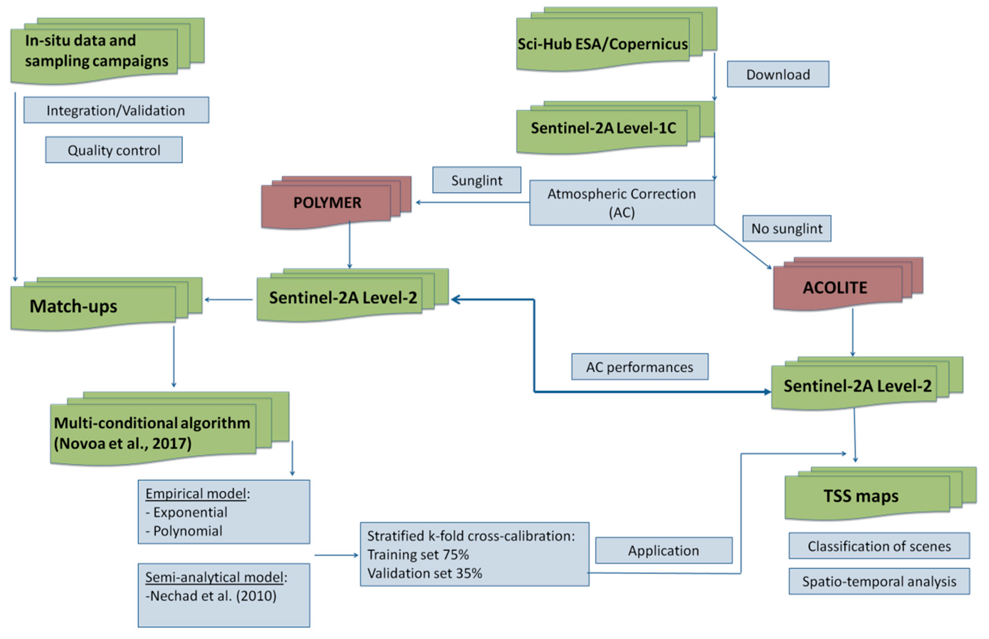
2. Materials and Methods
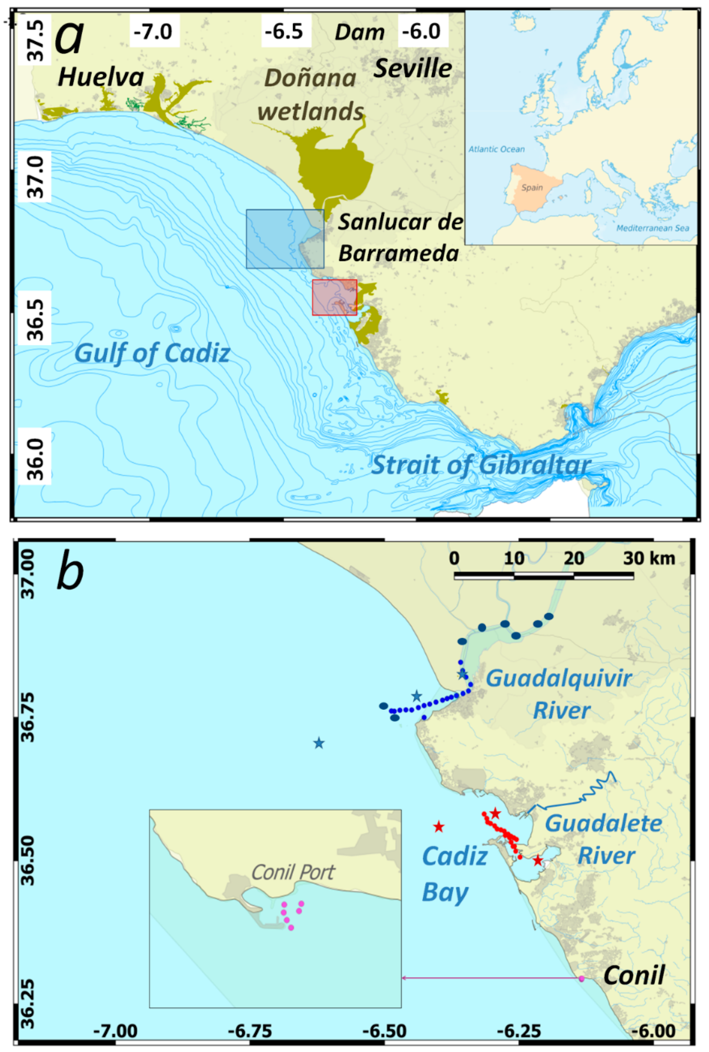
2.1. Study Area

The Spanish region of the Gulf of Cadiz is in the north-eastern Atlantic Ocean enclosed by the southern Iberian and northern Moroccan margins, where the Strait of Gibraltar is the natural and oceanographic border (Figure 1). The area includes the coast of the province of Huelva and the western region of the Cadiz coast (SW Iberian Peninsula). Along the littoral stretch of Cadiz there are several estuaries partly enclosed by spits and salt marshes, which are associated with the mouths of rivers, such as Guadalquivir and Guadalete (Figure 1). Specifically, the Guadalquivir estuary corresponds to one of the largest and most productive estuarine systems of Western Europe [25]. The estuary exhibits a semidiurnal meso-tidal regime extending 110 km inland from its mouth to the Alcalá del Río dam, the upstream tidal limit [39]. The river discharge, controlled anthropically by this dam, usually shows a pronounced dry/wet signal depending on rainfall, as well as large interannual variation [40,41]. This estuary presents several notable characteristics, including the largely protected estuary marshes forming part of the Doñana Natural and National Parks, which are a UNESCO-MAB Biosphere Reserve. The river between Sanlúcar de Barrameda and Seville is unique, being the only navigable river in Spain [42]. The estuary is strongly affected by human-related activities and has undergone rapid agricultural, fisheries, touristic, and anthropogenic developments, particularly in recent decades [43]. The seaward export of suspended material and nutrients from the river directly affects phytoplankton productivity, nutrient dynamics and the transport of pollutants in the coastal ocean [25,44]. From one point of view, intense turbid signals usually produce negative effects on water quality and clarity, major determinants of the productivity of an aquatic system, and of the tractability of water for human consumption, recreation and manufacturing [25,45]. Prolonged high-turbidity episodes originated hypoxia and inhibition of phytoplankton growth in the Guadalquivir coastal region [38], resulting in public concern [46]. From the other point of view, the sediment loads from the estuary also have positive impacts as key source of material and nutrients which greatly benefit the ecology and geomorphology of the estuary and adjacent regions [25,41,47].
Southeast of the estuary is the Natural Park of the Cadiz Bay, whose framework comprises a large semi-enclosed bay with characteristic low-coast morphology and a broad area of salt marshes. This region has recently been subject to severe anthropogenic pressure from increasing population density as well as from the aquaculture and other industries discharging into the bay [26]. The bay can be divided into four areas from a purely hydrological point of view: the outer bay to the north, the inner bay or barrier-island-lagoon to the south, the intertidal system of salt marshes to the south and southeast, and the terrestrial bay [26]. Sub-tidal and lower-intertidal vegetation has foreshore characteristics offering a rich and varied ecosystem which is of vital importance as the biotype for a multitude of organisms; although currently this is somewhat deteriorated due to human intervention [48]. The continental supplies come from the Guadalete River (Figure 1), from the tidal inlets and from the continuous mud transport from the marshes by ebb-currents. Human-induced development of the surrounding coastal areas associated with regular dredging, land disturbance, industry and tourism [49], in addition to wind- or tidal-driven sediment resuspension frequently result in pulsed, short-lived, turbidity episodes [50,51]. This environment, together with the Guadalquivir River, constitutes a significant source of sediment maintaining the sedimentary balance of the adjacent littoral area.

2.2. Sentinel-2 Imagery

Sentinel-2 scenes were downloaded from the Sentinel’s Scientific Data Hub (https://scihub.copernicus.eu/). These images corresponded to Level-1C (L1C) products at Top Of Atmosphere (TOA). In this study, the images from tile 29SQA (Sentinel-2 mission gridding system) were used. Only scenes with low cloud coverage were selected for further analysis (<60% cloud coverage). Since the first MSI image released at this location in November 2015, only a limited number of partially cloud free data was available (50%) due to the poor weather conditions. Therefore, a total of 23 images were selected during the study period from November 2015 to February 2017 (Table 1).

2.3. Atmospheric Correction Methodologies

The Sentinel-2A images were processed to Level-2A (L2A) data by using two different AC implementations (Table 1, Figure 2). Both processors were image-based, so no in-situ radiometric measurements were required. In practice, these corrections have major benefits for end user applications, which need direct satellite-derived water reflectance to assess water quality parameters.
The first AC corresponded to the analytical algorithm POLYMER [22]. This flexible algorithm was based on spectral optimization, but with a complex approach due to the necessity to use a wider range of spectral bands to estimate the atmospheric and sun-glint correction [22]. This spectral matching approach can thus perform AC in the sun-glint and retrieve the ocean color based on the idea that a flexible atmospheric model may fit the sun-glint signal, even if this signal is dominating and unpredictable. The output parameter obtained was water reflectance hereinafter referred as ρw (dimensionless) at 60 m spatial resolution.
The second tool used was based on the ACOLITE (20170718.0) processor developed by the Royal Belgian Institute of Natural Sciences (RBINS) supporting free processing of both Landsat-8 and Sentinel-2, specifically for aquatic applications [12,13]. Previous tests with VR-NIR AC failed in moderate- to high-turbidity regions due to incorrect estimation of the aerosol reflectance [17]. The SWIR bands at 1.6 and 2.2 μm were used by default for the aerosol correction, as they should be black over all water types [12,17]. In general, the use of this configuration for the aerosol correction over turbid waters is preferred, with a sub-scene or other locally representative, but fixed, epsilon value (aerosol type), improving the noise level in the products [13]. ACOLITE outputs were expressed as dimensionless water-leaving radiance reflectance or water reflectance in all visible and NIR bands and can compute a multitude of other parameters [17,20]. Data set was resampled to 10 m pixel size, whereas bands with 20 m and 60 m spatial resolution were replicated.
All the images were corrected with ACOLITE processor with masked pixels obtained during sun-glint scenes (Table 1). The images corrected with POLYMER corresponded to the four scenes of the field campaign dates due to sun-glint (27 May, 6 and 16 June 2016), in addition to 8 March and 24 September due to minimum cloud coverage over the study region (Table 1). Since the TSS multi-conditional model was develop using POLYMER-derived water reflectance estimations and subsequently applied on ACOLITE-derived products, a qualitative inspection of their performances was accomplished given the lack of in-situ radiometric measurements (no Aeronet-OC stations over the Gulf of Cadiz area). The inter-comparison was made over the same scenes on 8 March, 24 September, and 13 December 2016, and POLYMER strategy may be regarded as reference. We inspected ρw within three boxes in the Guadalquivir estuary (see location for blue stars in Figure 1) and Cadiz Bay (see location for red stars in Figure 1), extracted from the mean values of 5 × 5 pixels after correction with ACOLITE and POLYMER. The location ranged from offshore waters in the estuary at Box 1 (36.696°N, 6.676°W) to estuarine or turbid waters at Box 2 (36.773°N, 6.438°W) and Box 3 (36.811°N, 6.343°W), and from offshore the bay at Box 1 (36.571°N, 6.38°W) to turbid waters at Box 2 (36.55°N, 6.253°W) and Box 3 (36.503°N, 6.203°W) (Figure 1).

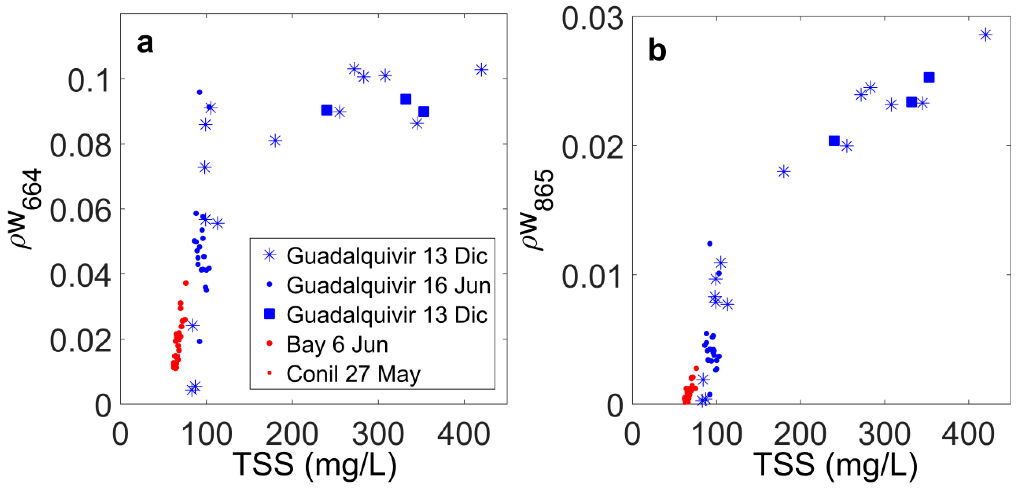
2.4. In-Situ TSS Data

Field campaigns during 2016 were conducted to calibrate and validate the TSS models (Figure 1, Table 1): Guadalquivir estuary (16 June and 13 December), Cadiz Bay (6 June) and Conil port (27 May). At each station, surface water samples were collected at the time of satellite overpass (~11:30 GMT), defining a maximum temporal window of 1 or 2 h [52] to prevent uncertainties associated with small-scale temporal variation, considering ESA acquisition plans (https://sentinel.esa.int/web/sentinel/missions/sentinel-2/acquisition-plans). For sampling, we moved in the boat to the edge of the water and inverted the sample container submerging it to a depth of 0.3 m below the water surface.
TSS were measured gravimetrically on preweighed Whatman GF/F filters after rinsing with distilled water according to the Joint Global Ocean Flux Study protocols JGOFS [53,54]. The filtered volume was 500 mL in all the samples. A total of 41 samples were finally selected from the Guadalquivir estuary and 24 from Cadiz Bay and Conil port for match-up purposes to develop the multi-conditional algorithm (See Figure 1 for spatial sampling at each site). In this work, TSS data match-ups between in-situ and corrected MSI scenes after POLYMER were performed by selecting mean water reflectance values over a 3 × 3 pixel window centered at the sampled location to avoid random noise. The minimum and maximum standard deviation of reflectance values encountered in the 3 × 3 boxes were 0.0005–0.0011 for the red and 0.0003–0.0009 for the NIR bands, respectively.

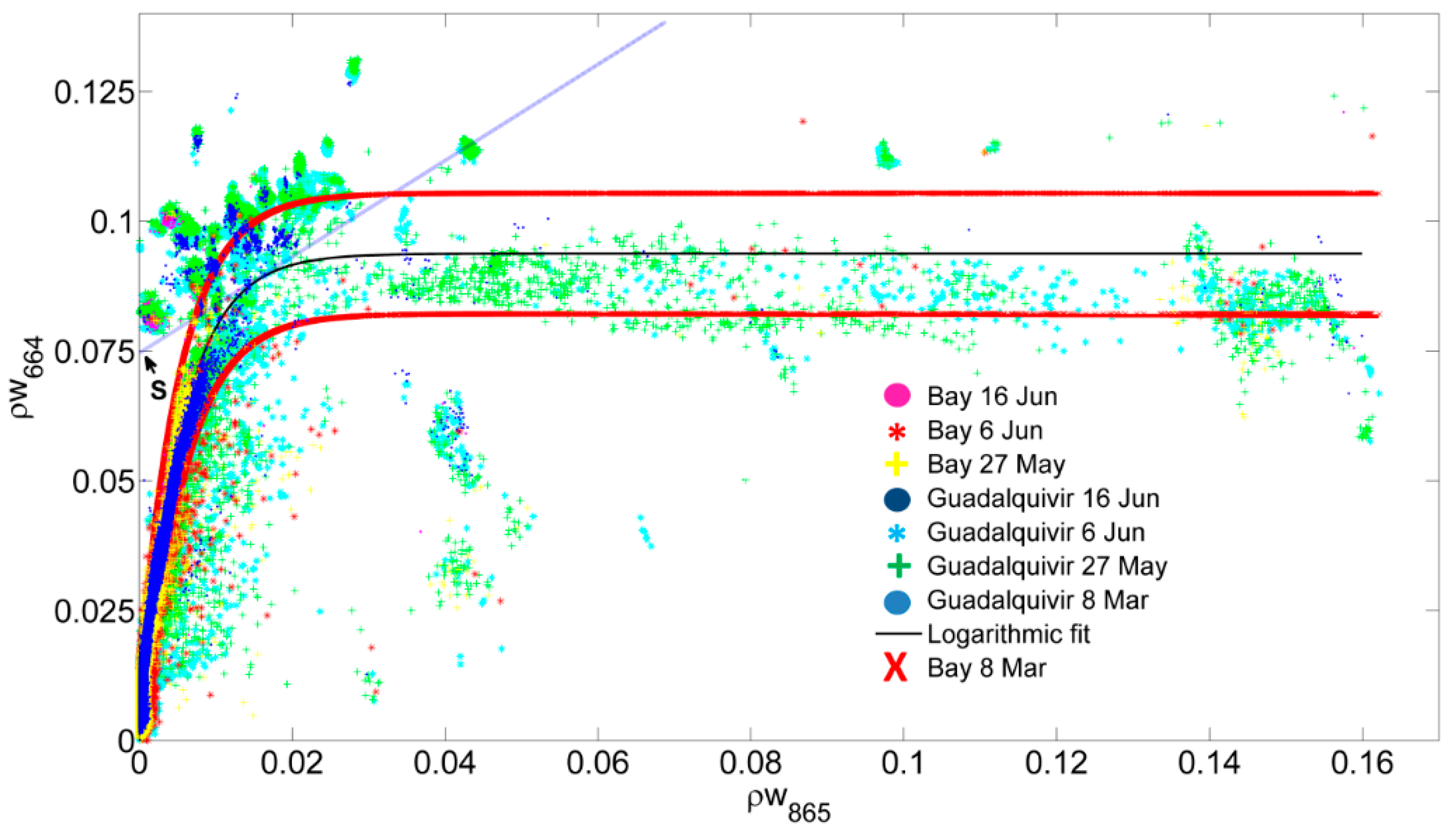
2.5. Selection of the Multi-Conditional TSS Algorithm

To adapt and regionalize a multi-conditional TSS model in the coastal region of Cadiz based on the methodology exposed in [37], an initial inspection of in-situ TSS and ρw (red and NIR) match-ups was conducted. Following the recommendation based on the application of the model without the need for field radiometric measurements [37], we conducted the switching bound selection approach with water reflectance after POLYMER correction. We compared ρw in the red and NIR to detect the saturation points, adjust the TSS model and infer the switching values in both Guadalquivir estuary and Cadiz Bay ROIs (Figure 1). The two bands selected for the algorithm were intended to be also used for Landsat-8 satellite. The red-to-NIR switching ρw values (S) were chosen based on the saturation of the most sensitive bands by means of band comparison. The data points were modeled by means of a logarithmic regression curve and the value of the saturation point was defined as the first derivative of the regression curve (the slope or tangent) equal to 1. The S transition value corresponded to the point of intersection between the tangent line on the regression curve where the slope is 1 and the y axis when S = ysat − xsat (ysat and xsat are the coordinates of the saturation point). In addition, the equations were weighted to ensure a smooth transition between both models for intermediate values. The smoothing bounds (S95+, S95−) were derived from the 95% confidence levels of the regression curve following the same procedure as for the S value calculation and using the weighted red-NIR equation: TSS = α TSS red + β TSS NIR, where α = ln(S95+/ρw665)/ln(S95+/S95−) and β = ln(ρw665/S95−)/ln(S95+/S95−).
Exponential and polynomial empirical models using the single bands of red and NIR were considered in this study for the Guadalquivir estuary. Additionally, the semi-analytical, non-linear model developed for turbid waters was also tested after recalibration with in-situ data [29]. This algorithm has already provided good performance in these coastal waters for DEIMOS-1 satellite [30]. The mathematical formulation of the model was defined as:
TSS = A ρ w 1 ρ w C + B
where: ρw corresponded to the water reflectance, C (dimensionless) was defined utilizing standard data computed from the literature (for the MSI red and NIR bands C was equal to 0.1728 and 0.2115, respectively [29]), B (mg/L) represented measurement errors in both reflectance and TSS, and A (mg/L) was the calibration parameter relating reflectance to TSS. For this analysis, the coefficients A and B were derived by non-linear robust weighted regression to find the best-fit values. This robust fitting procedure was insensitive to outliers. To improve the fit, considering the log-normal distribution of TSS, we utilized the Cauchy Weight Function (w) as w = 1/(1 + res2), where res is the residual.
Stratified k-fold cross-validation (k corresponded to the disjoint subsamples or folds) was applied to assess the accuracy of the model predictions, i.e., the models were calibrated using a subset of the data (training set, 75% observations) and the model predictions evaluated using an independent data set (validation or test set. 35% observations) assigned using stratified-random selection [55]. This assignment was repeated 100 times with the condition that the test set could not overlap. For each fold, the model was calibrated using the training data set and the prediction was compared to the test set, allowing derivation of the accuracy of satellite-derived TSS. The performance of each model was assessed using the Pearson coefficient of correlation (r), the bias (mg/L) and the normalized root mean square error (NRMSE, in %). A final assessment of the accuracy of model prediction was derived by averaging the error statistics over all folds. Subsequently, the definitive calibration parameters A and B were calculated for each model with all 41 samples. After model adjustment, the semi-analytical algorithm was applied to the atmospherically corrected scenes to generate the time series of Sentinel-2A along this region (see detailed flow chart in Figure 2).

3. Results

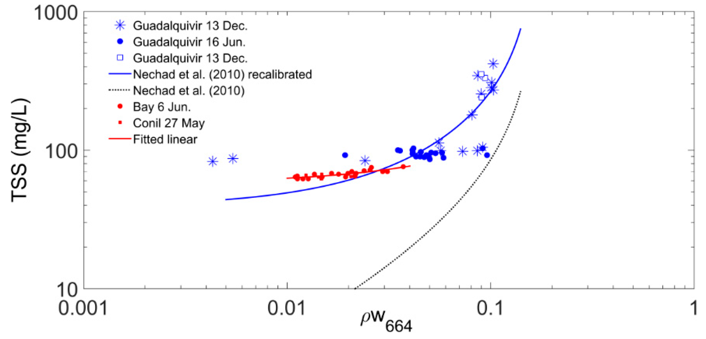
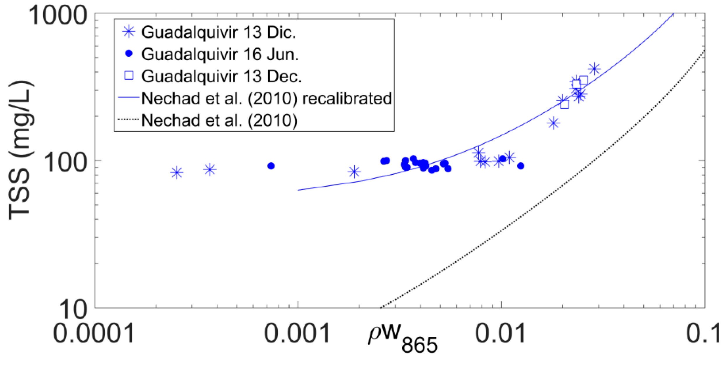
3.1. Multi-Conditional Algorithm

The scatter of TSS measurements against ρw in the red (B4, 664 nm) and NIR (B8a, 865 nm) bands for the Guadalquivir estuary, Cadiz Bay, and Conil port is presented (Figure 3). The concentration of in-situ TSS varied from 80 to 420 mg/L in the estuary and from 60 to 78 mg/L in both Cadiz Bay and Conil port. The highest values were measured in the Guadalquivir estuary on 13 December 2016, upstream of the estuary. The hydraulic regime during 16 June and 13 December 2016 was tidally-dominated (discharge from Alcalá del Río dam <40 m3/s) with no precipitation. There was a relationship between the red band and TSS concentration lower than 150 mg/L in the Guadalquivir estuary; and above this saturation was observed (Figure 3a). The NIR band appeared to be less sensitive to variations of TSS below 150 mg/L but showed sensitivity above this value (Figure 3b).
The equations after calibration with the fits and model prediction error for the red (Table 2) and NIR (Table 3) bands are presented. The recalibrated model displayed the best correlation (0.794, and 0.974) and minimum bias (0.81, and 0.57 mg/L) for red and NIR bands, respectively. Similar results were found for the empirically-derived exponential and second order polynomial algorithms (Table 2 and Table 3). The advantages of the semi-analytical algorithm relied on its strong theoretical background, taking into account assumptions about spatial and temporal variability of specific inherent optical properties (IOPs) and its simple application to multiple bands of any ocean color sensor [29]. Therefore, the combination of the semi-analytical algorithms using the red and NIR bands was selected to define the multi-conditional model using a radiometric switching criterion. The recalibrated algorithm for the red and NIR bands is presented (Figure 4 and Figure 5), as well as the original fit at those wavelengths [29]. In Cadiz Bay and Conil port, a linear model based on the red band was selected (r = 0.91, p < 0.001; TSS = 466 × ρw664 + 58). Due to the low number of measurements and small range of TSS concentrations (60–80 mg/L), the NIR model for the estuary was also applied in those regions.
The scatter plot between MSI-derived water reflectance values in the red and NIR bands extracted for the Guadalquivir estuary and Cadiz Bay ROI (Figure 1) during scenes acquired on 8 March, 27 May, and 6 and 16 June 2016 is presented (Figure 6). The red-to-NIR switching ρw values (S) were chosen based on the saturation of the most sensitive bands by means of band comparison. The smoothing bounds (S95+, S95−) were derived from the 95% confidence levels of the regression curve (Figure 6). The transition and intervals selected for the red-to-NIR multi-conditional algorithm were summarized (Table 4).

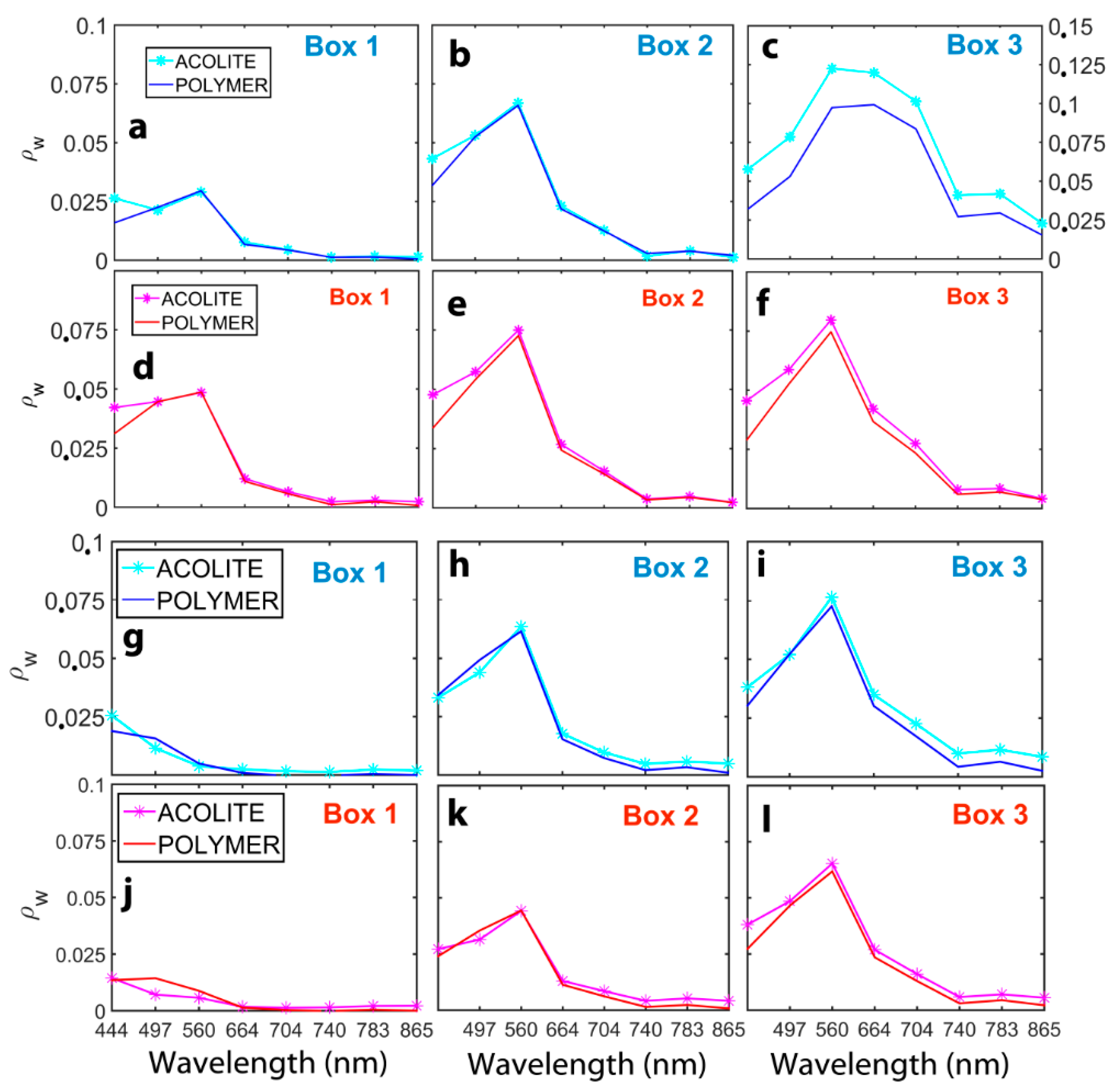
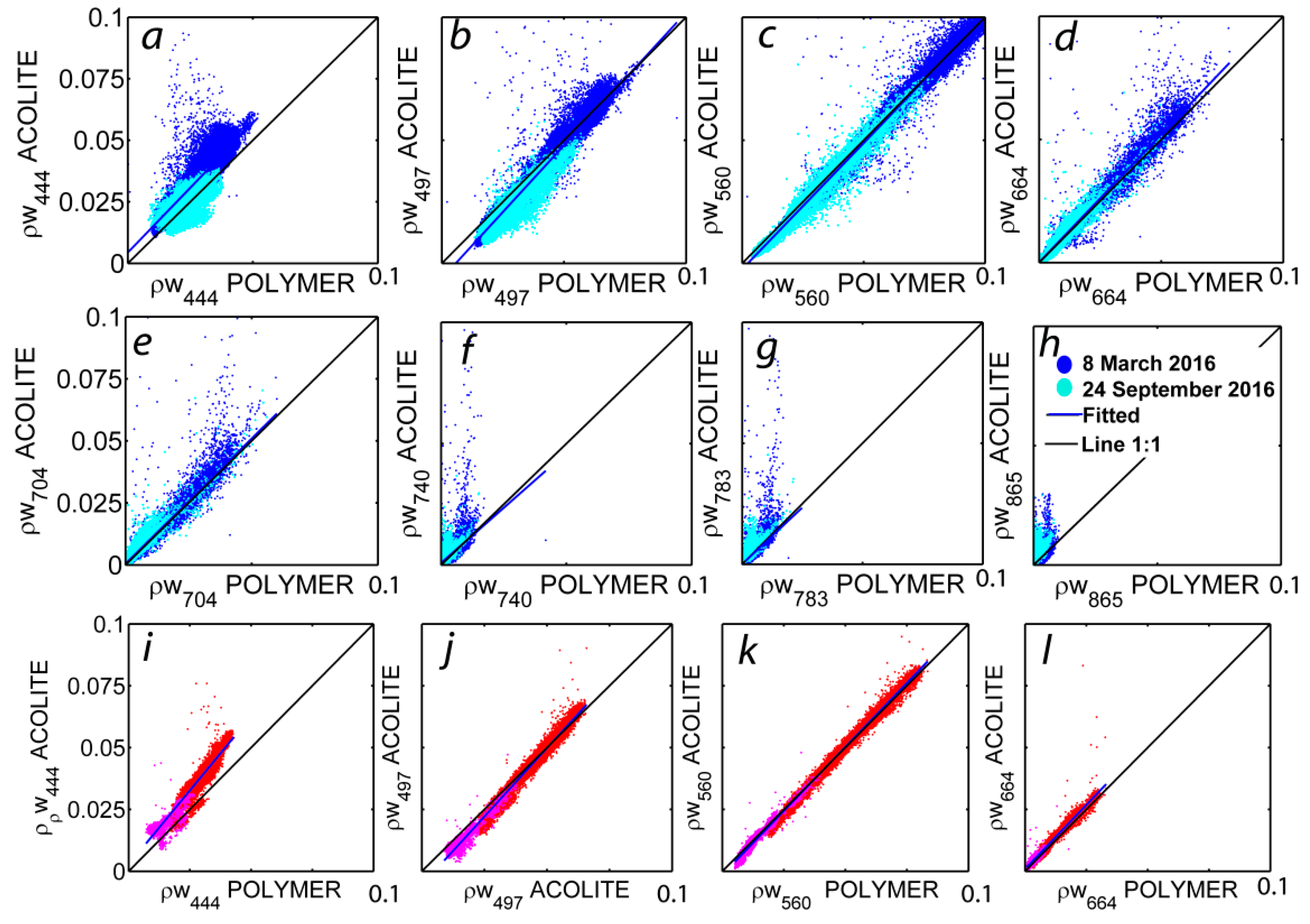
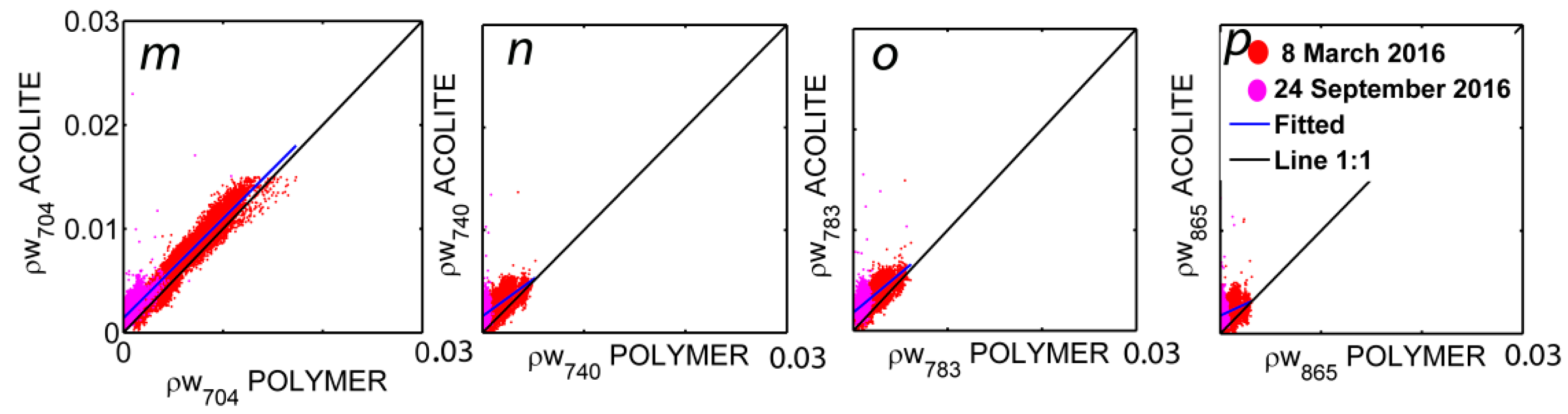
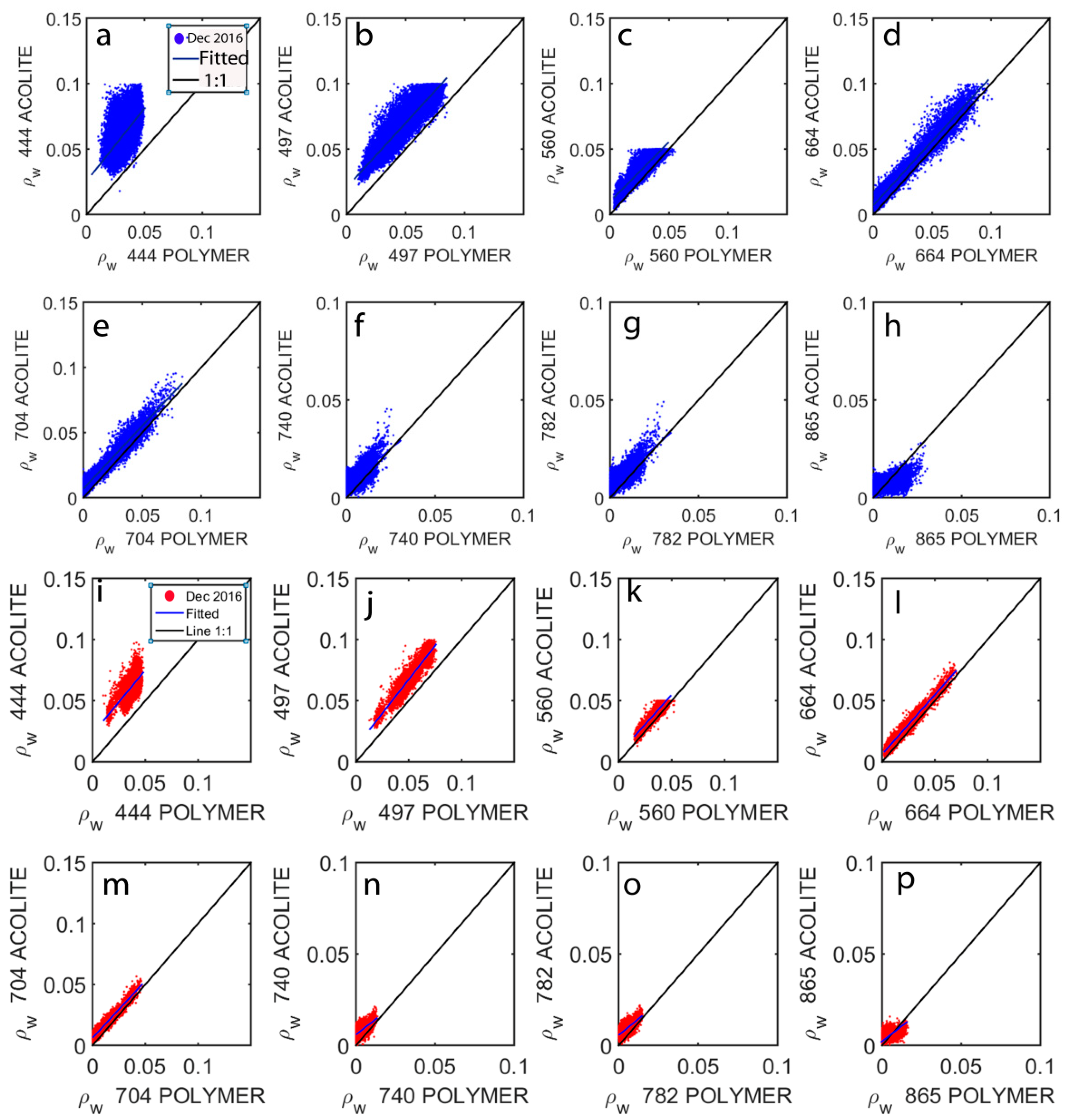
3.2. Analysis of the Atmospheric Correction Strategies

Water reflectance spectra (ρw) for three boxes in the Guadalquivir estuary and Cadiz Bay was extracted from the mean values of 5 × 5 pixels (Figure 1) after correction with ACOLITE and POLYMER on 8 March and 24 September 2016 (Figure 7). Minimum differences can be observed between ACOLITE and POLYMER. The inspection showed ρw values ranging from clear offshore conditions to moderately turbid conditions in the estuary and bay, with similar spectral signatures for each AC. A strong reflectance peak in the green part was observed at both locations. In addition, Boxes 3 exhibited higher ρw on all bands, assumed to be related to larger TSS levels within these regions. Additionally, a comparison between both AC strategies was carried out in the Guadalquivir and Cadiz ROI (Figure 1) for the two scenes with minimum cloud coverage over the study region (8 March and 24 September 2016) and for the scene with in-situ sampling (13 December 2016). The results exposed similar performances in the visible and NIR spectrum between ACOLITE and POLYMER (Figure 8 and Figure 9), showing high Pearson coefficients of correlation for the visible bands with slightly lower correlation in the red-edge and NIR bands (Tables S1 and S2 in Supplementary Material).
Severe impact of sun-glint at these latitudes limited the number of images by ACOLITE, which is not adapted yet to perform sun-glint correction. An example on 27 May 2016 with the presence of sun-glint over the entire coastal region in the true-color Red-Green-Blue (RGB) composite (B4-B3-B2) and in the water reflectance at 664 nm (B4) after ACOLITE AC is presented (Figure S7 in Supplementary Material). Particularly, images from May until September were influenced by intense sun-glint over the littoral region of Cadiz (Table 1). This concern prevented the effective use of ACOLITE, thus decreasing the temporal MSI coverage without any data in many areas.

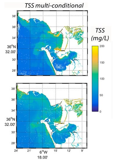
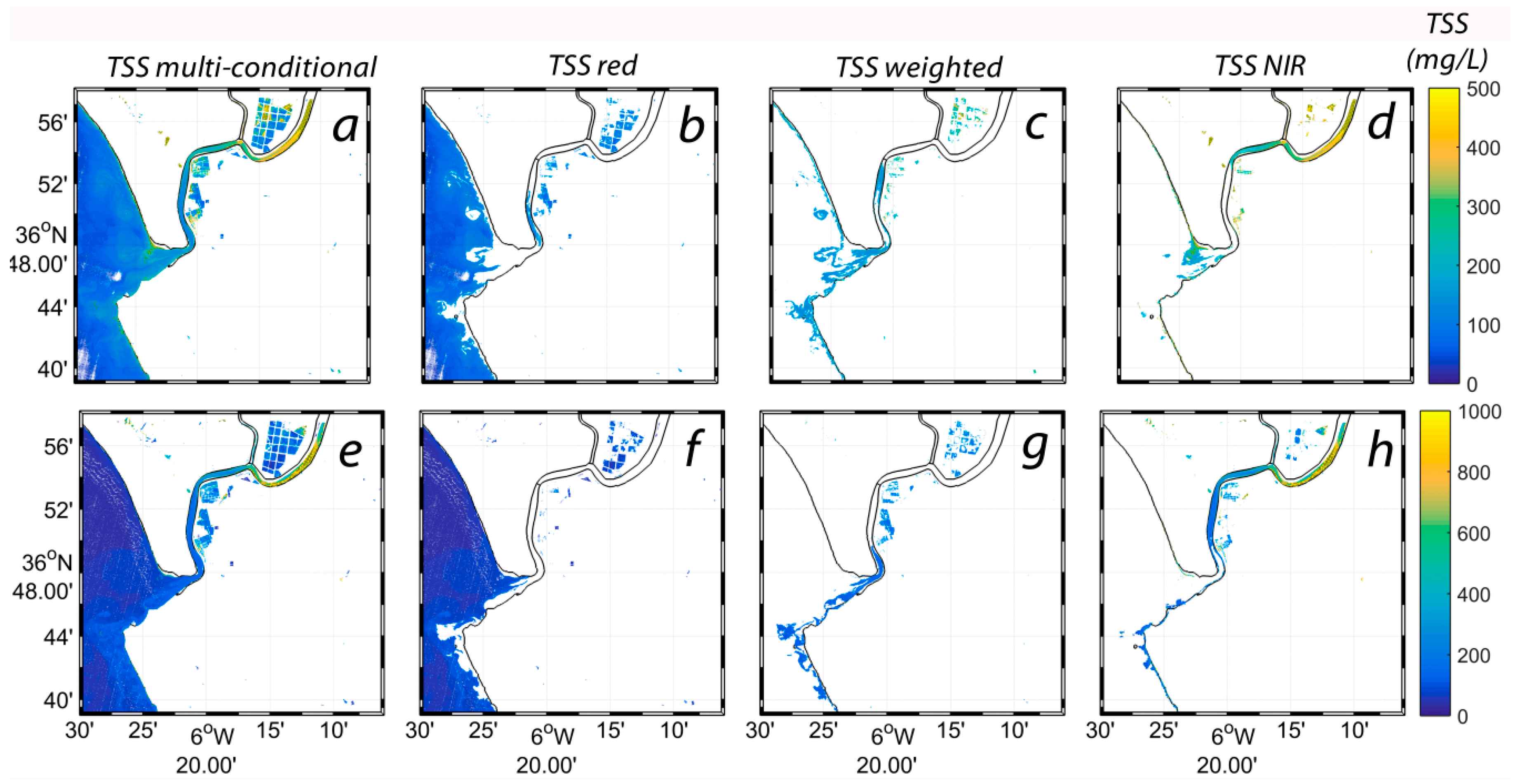
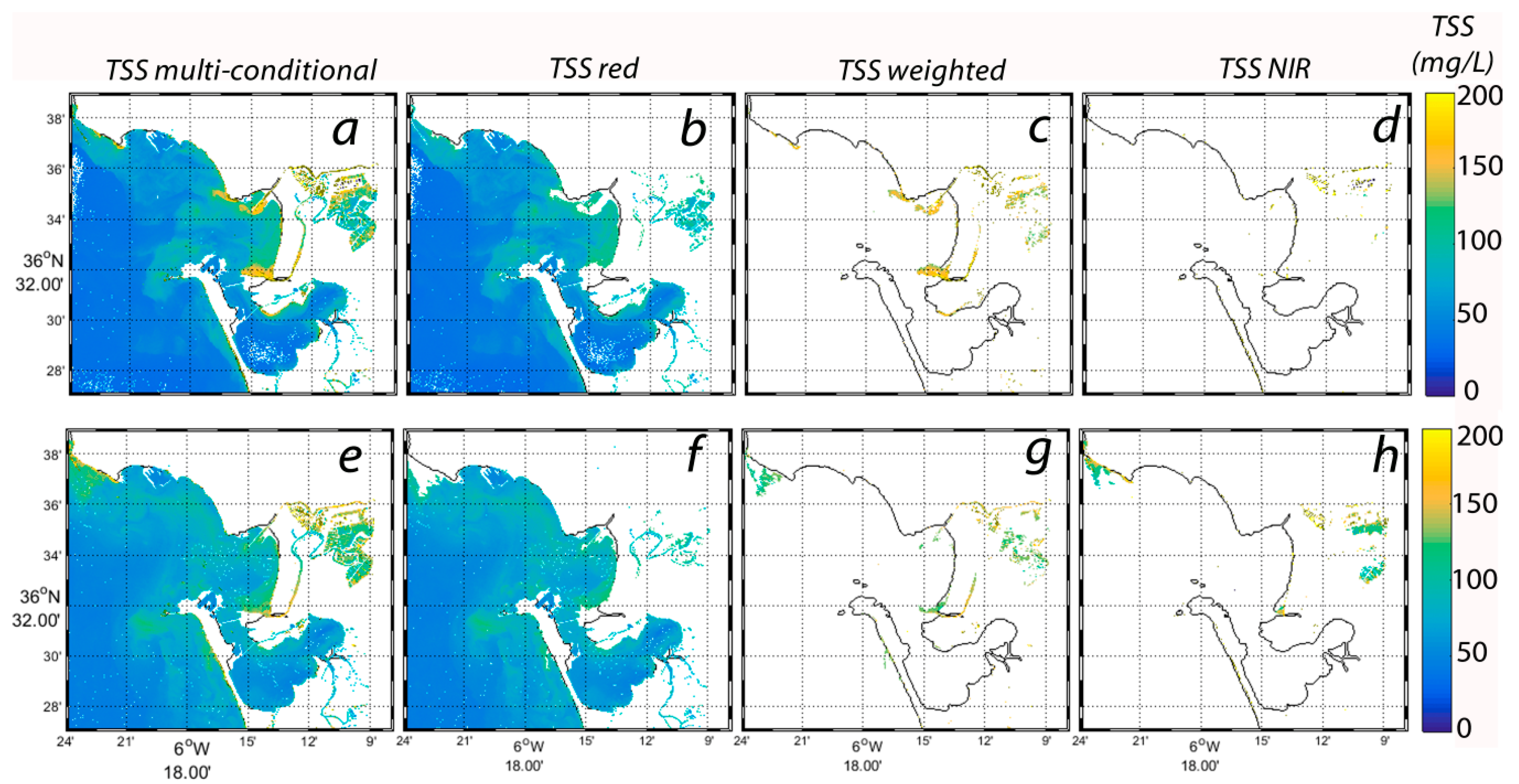
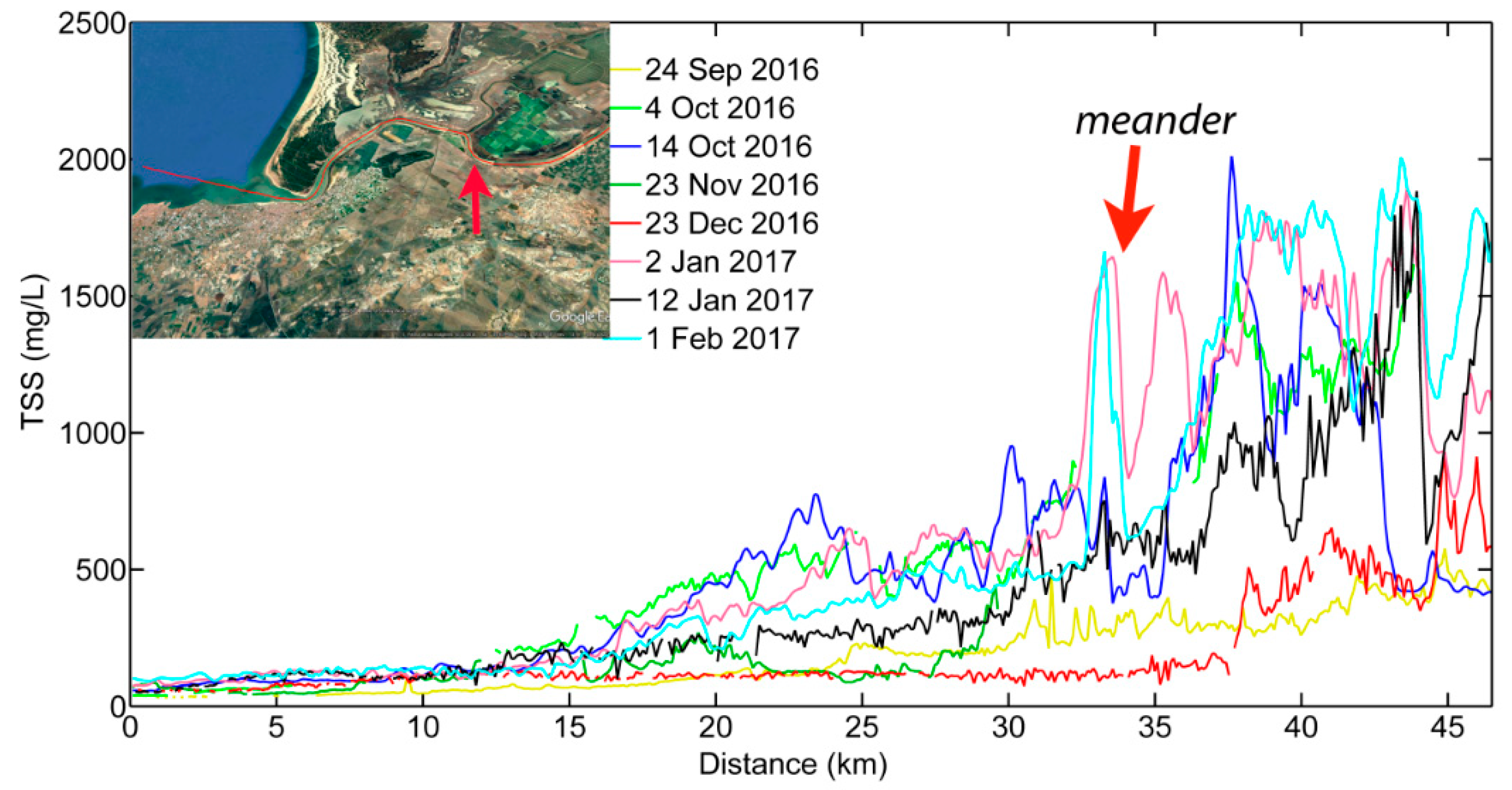
3.3. Application of the TSS Multi-Conditional Algorithm

An example of the application of the switching TSS model combined with the smoothing procedure to a cloud- and sun-glint-free MSI image acquired over the Guadalquivir estuary on 19 December 2015 after ACOLITE AC at 10 m spatial resolution is presented (Figure 10). Daily freshwater discharge from Alcalá del Río dam during previous days was <40 m3/s (tidally-dominated state) with nonexistent precipitation. Figure 10a shows the final TSS concentration whereas Figure 10b–d presents TSS calculated using the red recalibrated, weighted and NIR recalibrated models (Table 4). The smooth transition between the remotely sensed TSS concentrations was clearly noted along the mouth of the estuary as an increment in TSS. The multi-conditional algorithm switches were clearly observed: beginning with the estimation of TSS using the red band (664 nm) with the confinement of the relatively clear waters offshore, followed by the weighted model within the mouth of the river and a first transect of the channel to the final application of the NIR band upstream. At this spatial coverage, turbidity features were enhanced in detail as well as the spatial TSS concentration along the river channel. The external TSS with low concentrations (<250 mg/L) have been characterized given the low input of freshwater discharge during tidally-dominated cycles [56], similar to those reported during this scene (Figure 10a). The 10 m pixel size is a great advantage in coastal monitoring, focusing on the feasibility to analyze TSS gradients within the estuary and along the navigation channel. In this regard, a constant TSS increment was observed towards the upper part of the estuary, with the definition of the Estuarine Turbidity Maximum (ETM) at a meander located at the Brazo de la Torre site (Figure 11) and upstream (400–500 mg/L). Another example of TSS mapping estimated with the multi-conditional algorithm on 17 February 2016 (tidally-dominated estuarine regime and no precipitation) is presented (Figure 10e). The overall concentration increased longitudinally from offshore to upstream, exhibiting higher TSS values than Figure 10a mainly upstream of the channel. In this case, the ETM was also observed in the same region but with higher magnitude (~900 mg/L), clearly indicating highest concentrations tended to be located around 30 km from the estuary mouth. These findings agreed with in-situ observations carried out in the estuary [38], where TSS concentration ranged from 500 to 2500 mg/L along this transect of the river channel.
The spatial frame of the Sentinel-2 imagery allowed us to examine TSS along a section within the river channel, illustrating the TSS spatio-temporal distribution. Eight longitudinal TSS transects (47 km) along the estuary were displayed between autumn and winter 2016–2017 (Figure 11). The images at 10 m spatial resolution were selected after ACOLITE procedure with no sun-glint issues and minimum cloud coverage. Imagery were acquired over a similar range of hydrological conditions corresponding to the tidally-dominated estuarine regime with discharge from Alcalá del Río dam <40 m3/s during the previous three days, but spanning different tidal conditions, thus leading to distinct tidal currents and associated resuspension processes (Table S3 in Supplementary Material). The overall concentration longitudinally increased from offshore to upstream along transects, exhibiting different spatial fluctuations mainly associated to the tidal conditions. TSS surface concentration showed variations associated with diverging sedimentary patterns, such as the enhanced TSS presented along the entire channel during spring tides (4/14 October 2016, 2/12 January, and 1 February 2017). On the contrary, minimum values were recorded through neap tides (24 September, 23 November and, 23 December 2016) at the final transect of the estuary. This stretch was also characterized by two adjacent low radius curvature bends that further enhanced secondary flow, contributing to the maintenance of high turbidity levels [25], as can be observed in the maps (Figure 10). The temporal changes of the ETM and its magnitude could be examined along the section, with noticeable features mainly depending on tidal cycle similar to model predictions [41]. Previous works, by means of in-situ and model data, have described similar TSS patterns along the river channel specifically during low river discharge [25,38,57].
In addition, the map of TSS after the application of the multi-conditional model in Cadiz Bay is presented on 19 December 2015 and 17 February 2016 (Figure 12). In this case, lower TSS values were encountered in the region highlighting TSS concentration was mostly determined utilizing the red model. The weighted model was used over the areas with higher TSS and along the coast. The discharge from the Guadalete River can be observed such as small plumes with high TSS concentration. Small-scale variability was exhibited, such as the turbid features spreading out of the inner and outer bay and the streaks of sediments along the coast probably due to wind or tidal-induced particle resuspension and enhanced sediment erosion and resuspension by nearby mudflats [26]. Small-scale sediment transport can be observed downstream from the offshore regions, permitting the appraisal of sediment dynamics from the bay to the adjacent regions.

4. Discussion

The deviation between the calibrated fit and the original semi-analytical algorithm (Figure 4 and Figure 5) could be related to AC model issues such as the overcorrection of red/NIR bands by POLYMER, specifically during high glint scenes as the ones corresponding to the sampling dates in May and June 2016. To inspect this, we included the signal separation between atmosphere and water of all the Sentinel-2A images corrected with POLYMER (Figures S1–S6 in Supplementary Material). The maps represented the water reflectance (ρw) and atmospheric reflectance (ρatm) of the red and NIR bands used for the calibration of the multi-conditional model. The atmospheric reflectance corresponded to the atmospheric component and sun-glint, not including the Rayleigh scattering. Sun-glint affected June (in-situ sampling, Figures S3 and S4) and September (Figure S5) scenes, whereas March (Figure S1) and December (in-situ sampling, Figure S6) imagery showed little sun-glint. In this case, Sentinel-2A images indicated the glint effect increased towards the east. Examination of the water and atmosphere decoupling showed water patterns were only marginally visible in the atmospheric signal. The scatter for TSS concentrations close to 100 mg/L and low ρw values was encountered in both scenes in the Guadalquivir estuary (16 June and 13 December 2016), suggesting the variability barely increased with sun-glint. A methodology for assessing AC processors based on in-situ measurements by the Ocean Color Climate Change Initiative (OC-CCI) has been examined concluding that glint affected pixels were only marginally deteriorated compared to the non-glint pixels in POLYMER products [58]. Another possible reason of this scatter could be related to the modification of water reflectance values due to adjacency effects. POLYMER corrected adjacency effect simultaneously with AC using the polynomial model and several studies indicated it worked out accurately (both on simulated data and actual imagery), with ice adjacency but also vegetation or dry land adjacency [22,58,59].
Based on mineralogical studies, abundant silt and clay mineral fractions were found either in the Guadalquivir estuary, or in the adjacent continental shelf corresponding to river inputs, where most of them were detritus with a small portion being diagenetic [60,61]. It has been characterized that 100 mg/L was the minimum TSS found in the estuary mouth during summer time and tidally-dominated regime, with mean and maximum concentration of 600 and 2000 mg/L, respectively [38], establishing a robust relationship between TSS and turbidity for this wide range of concentrations [54]. The different sediment types and concentrations varying seasonally along the estuary could also affect the offset between the original [29] and the regional calibrated algorithm. The same characteristic was found in the estuary applying the NIR band of Deimos-1 satellite to estimate TSS [30,62], with an overall deviation between the original and the regional calibrated model pointed out in the range of TSS varying between 100 to 1000 mg/L [30].
The preliminary efforts of this research exhibited the promising capability of Sentinel-2A to support coastal management as a valuable tool for TSS monitoring. The switching method allowed a smooth transition between the remotely sensed TSS from the offshore low-turbidity waters to the moderate- and high-turbidity waters inside the bay and estuary. This avoided saturation issues shifting towards longer wavelengths while increasing concentration of TSS associated with the specific inherent optical properties of the suspended particles [63,64]. The results illustrated the importance of applying the multi-conditional algorithm over areas with a wide range of TSS concentrations associated with both temporal and spatial variability, which better estimated TSS than a simple model in the visible or NIR part of the spectrum. Nonetheless, additional insights must be considered for inspection of a wider range of TSS concentrations and other water quality parameters (chlorophyll-a, Colored Dissolved Organic Matter) to establish a continuous framework for the ongoing services relying on both Sentinel-2 twin satellites.
Both ACOLITE and POLYMER provided similar performance in the visible and NIR spectrum after inter-comparison due to in-situ data on water reflectance was not available. Specifically, sun-glint restricted the number of usable images during late spring and summer scenes using ACOLITE. On the contrary, the results confirmed that the flexible POLYMER was able to address intense sun-glint effects, since the algorithm was originally developed to process MERIS data in glitter-affected areas. Sentinel-2 processing with POLYMER is rather new and is expected to evolve in the near future. The state of the art of Landsat-8 and Sentinel-2 satellites has been recently outlined evidencing a new algorithmic challenge was required in order to remove and filter sun-glint effects [13]. These concerns can be addressed using a flexible algorithm such as POLYMER, which does not use a specific aerosol model, but fits atmospheric reflectance and sun-glint with a polynomial [22]. The robustness of POLYMER to the effects of the sun-glint and semi-transparent clouds led to a large gain of spatial coverage [22,65]. The improvement of ocean color remote sensing in the Arctic revealed that POLYMER was robust when pixels were contaminated by sea ice and estimates of water reflectance showed better agreement with in-situ measurements [59]. The OC-CCI project updated AC and in-water algorithms including POLYMER to allow both enhanced coverage and quality in case-2 waters. Novel algorithms, which include sun-glint correction, should expect to increase coastal coverage substantially, leading to improved information about the temporal variability of biophysical processes. Future insights are required to establish up-to-date information about the different AC strategies to correct MSI imagery, with an increasing demand for guidelines and recommendations by the international ocean color community and particularly, by end users and water managers. However, in-situ and satellite radiometric match-ups would be necessary to draw further conclusions regarding the accuracy of both AC over this coastal region.
This research established that the regular monitoring of TSS, within the scales of human activity impacts (10 m), could be accomplished in several environments. The great benefit of this spatial resolution was highlighted; images showed detailed features suggesting the feasibility of mapping TSS in ports, estuaries, and river channels. These results are encouraging for research, as well as can sustain the challenge to assist the demanding task to support water quality monitoring, validation of sediment transport models, dredging operations, maritime defense, and fisheries practices. Specifically, this emerging information will be attractive for several studies relying on sediment dynamics such as hydro-morphological analysis [66]. The plausibility of incorporating Sentinel-2 data within the modelling for operational use will enhance the examination of the concentrations, fluxes, and transport of material, as well as the morphodynamic balance of the systems. With both Sentinel-2A and -2B in operation, research will be globally afforded at five-day revisit time at the Equator. This will be beneficial for numerous applications to implement routine water monitoring and management plans required for sustainable development and document the response of the coastal ecosystem to environmental changes. Considering the high frequency of cloudy data or sun-glint over this region, the inclusion of Sentinel-2B will increase the amount of high-resolution imagery to improve understanding of any spatio-temporal variability. In addition, the mission is also close to the Landsat-8 local times, allowing the seamless combination of Sentinel-2 data with historical images to build long time series [16]. The possibility of using other similar satellites such as Landsat-8 to complete the temporal coverage at these coastal scales would provide researchers, policy makers and end users with insights on important ecosystem dynamics and their relationship with climate change [67]. The geostationary sensors, which will offer the basis for future superior temporal coverage of TSS monitoring, must provide several images per day compared to once per day of the standard ocean color satellites. It has been demonstrated, using the Spinning Enhanced Visible and Infrared Imager (SEVIRI) geostationary platform (images every 15 min), the great possibilities for examination of high frequency dynamics of the coastal regions [68]. Additional initiatives must be focused on the continuity of EO services relying on high-resolution optical observations to establish a continuous framework for supporting scientists and ecosystem policy-makers. This evaluation would contribute to consolidate MSI image-based techniques for operationally and routinely dissemination, as they require to be reinforced before being able to actively support coastal zone management as contribution to the Copernicus programme.

5. Conclusions

This study is one of the first attempts to test the capabilities of Sentinel-2A satellite in high-turbidity waters during its first year of operational service. High-resolution imagery (10 m) from MSI is used to quantify TSS concentrations in the Guadalquivir estuary, Cadiz Bay and adjacent waters. The work provides the application of a multi-conditional algorithm to estimate TSS over a wide range of concentrations, using water reflectance of the red (664 nm) and NIR (865 nm) bands after atmospheric correction with POLYMER and ACOLITE strategies. The results present a favorable approach with a smooth transition between different TSS models, highlighting the benefit of these emerging methodologies over coastal and estuarine waters. Our assessment represents a preliminary study that can be applied to other turbid environments worldwide to address saturation issues in the visible bands. The possibility of detecting the maximum turbidity zone along the estuary is demonstrated, underlining the complex spatio-temporal variability of turbidity patterns over these nearshore waters. Therefore, Sentinel-2A can address small-scale water monitoring due to the higher spatial and spectral resolution, suggesting its great potential even though it was not designed for aquatic applications. However, we suggest an extensive program of calibration/validation efforts over different coastal and inland waters and atmospheric conditions to advance Sentinel-2 twin mission status and establish up-to-date information about MSI’s capabilities.

Supplementary Materials

The following are available online at https://www.mdpi.com/2072-4292/10/7/982/s1, Figure S1: Maps of signal separation of atmosphere (ρatm) and water (ρw) for red (665 nm) and NIR (865 nm) bands, respectively. Sentinel-2A image of 8 March 2016 with POLYMER AC model (60 m); Figure S2: Maps of signal separation of atmosphere (ρatm) and water (ρw) for red (665 nm) and NIR (865 nm) bands, respectively. Sentinel-2A image of 27 May 2016 with POLYMER AC model (60 m). In-situ sampling was carried out during this day; Figure S3: Maps of signal separation of atmosphere (ρatm) and water (ρw) for red (665 nm) and NIR (865 nm) bands, respectively. Sentinel-2A image of 6 June 2016 with POLYMER AC model (60 m). In-situ sampling was carried out during this day; Figure S4: Maps of signal separation of atmosphere (ρatm) and water (ρw) for red (665 nm) and NIR (865 nm) bands, respectively. Sentinel-2A image of 16 June 2016 with POLYMER AC model (60 m). In-situ sampling was carried out during this day; Figure S5: Maps of signal separation of atmosphere (ρatm) and water (ρw) for red (665 nm) and NIR (865 nm) bands, respectively. Sentinel-2A image of 24 September 2016 with POLYMER AC model (60 m); Figure S6: Maps of signal separation of atmosphere (ρatm) and water (ρw) for red (665 nm) and NIR (865 nm) bands, respectively. Sentinel-2A image of 13 December 2016 with POLYMER AC model (60 m). In-situ sampling was carried out during this day; Figure S7: Sentinel-2 image on 27 May 2016 after ACOLITE correction showing moderate sunglint issues on the: (a) true-colour Red-Green-Blue (RGB) composite (B4-B3-B2), (b) water reflectance (ρw) at 664 nm (B4). Standard ACOLITE flags were used with masked pixels for sunglint; Table S1: Performance indicators of the comparison between atmospherically corrected spectra at different wavelengths by POLYMER and ACOLITE procedures in the Guadalquivir estuary and Cadiz Bay Region of Interest (ROI) on 8 March and 24 September 2016. Pearson coefficient of correlation (r), Root Mean Square Error (RMSE) and bias displayed. Parameters a and b correspond to the values of the linear fit both intercept and slope, respectively; Table S2: Performance indicators of the comparison between atmospherically corrected spectra at different wavelengths by POLYMER and ACOLITE strategies in the Guadalquivir estuary and Cadiz Bay Region of Interest (ROI) on 13 December 2016 (coincident with in-situ sampling). Pearson coefficient of correlation (r), Root Mean Square Error (RMSE) and bias displayed. Parameters a and b correspond to the values of the linear fit both intercept and slope, respectively; Table S3: Date and timing (UTC) of Sentinel-2A data acquisition, mean discharge (three previous days) from Alcalá del Rio dam (m3/s), mean precipitation (three previous days) at Sanlúcar de Barrameda (mm), tidal amplitude, and timing of low and high tides at the Bonanza tidal Gauge in Sanlúcar de Barrameda.

Author Contributions

I.C. and G.N. designed the study; F.S. performed the POLYMER processing; I.C. analyzed and interpreted the data; I.C. wrote the manuscript. All authors discussed the results and contributed to the manuscript.

Acknowledgments

We would like to thank the ESA and the Copernicus programme for distributing the Sentinel-2 data used in this study. Thanks to Quinten Vanhellemont for his assistance in using ACOLITE processor. We thank the Junta de Andalucía for the in-situ data archives: the Regional Water Management Agency (http://www.chguadalquivir.es/saih/) and the Regional Agroclimatic Station Network (http://www.juntadeandalucia.esagriculturaypesca/ifapa/ria/servlet/FrontController), as well as Puertos del Estado (http://www.puertos.es/). We acknowledge the CSIC Sampling Unit OPECAM (http://www.icman.csic.es/en/facilities/opecam-field-unit/) and Josefa Perez dredging ship for the campaign assistance. Isabel Caballero was supported by a postdoctoral grant from the Junta de Andalucía fellowship program. This work was financially supported by the Junta de Andalucía Projects P09-RNM-4853 and PR11-RNM-7722, PIE 201530I012 and the National Project CTM2014-58181-R. The authors acknowledge the anonymous reviewers, whose comments helped to greatly improve an earlier version of this manuscript.

Conflicts of Interest

The authors declare no conflict of interest.

References

  1. Halpern, B.S.; McLeod, K.L.; Rosenberg, A.A.; Crowder, L.B. Managing for cumulative impacts in ecosystem-based management through ocean zoning. Ocean Coast. Manag. 2008, 51, 203–211. [Google Scholar] [CrossRef]
  2. Becker, A.; Whitfield, A.K.; Cowley, P.D.; Järnegren, J.; Næsje, T.F. Potential effects of artificial light associated with anthropogenic infrastructure on the abundance and foraging behavior of estuary-associated fishes. Appl. Ecol. 2013, 50, 43–50. [Google Scholar] [CrossRef]
  3. Ouellette, W.; Getinet, W. Remote sensing for marine spatial planning and integrated coastal areas management: Achievements, challenges, opportunities and future prospects. Remote Sens. Appl. Soc. Environ. 2016, 4, 138–157. [Google Scholar] [CrossRef]
  4. International Ocean-Colour Coordinating Group. Mission Requirements for Future Ocean-Colour Sensors; McClain, C.R., Meister, G., Eds.; IOCCG Report 13; International Ocean-Colour Coordinating Group: Dartmouth, NS, Canada, 2012; p. 106. [Google Scholar]
  5. Cloern, J.E. Turbidity as a control on phytoplankton biomass and productivity in estuaries. Cont. Shelf Res. 1987, 7, 1367–1381. [Google Scholar] [CrossRef]
  6. Malenovský, Z.; Rott, H.; Cihlar, J.; Schaepman, M.E.; García-Santos, G.; Fernandes, R.; Berger, M. Sentinels for science: Potential of Sentinel-1, -2, and-3 missions for scientific observations of ocean, cryosphere, and land. Remote Sens. Environ. 2012, 120, 91–101. [Google Scholar] [CrossRef]
  7. Du, Y.; Zhang, Y.; Ling, F.; Wang, Q.; Li, W.; Li, X. Water bodies’ mapping from Sentinel-2 imagery with modified normalized difference water index at 10-m spatial resolution produced by sharpening the SWIR band. Remote Sens. 2016, 8, 354. [Google Scholar] [CrossRef] [Green Version]
  8. Dörnhöfer, K.; Gege, P.; Pflug, B.; Oppelt, N. Mapping indicators of lake ecology at lake Starnberg, Germany—First results of Sentinel-2A. In Proceedings of the Living Planet Symposium 2016, Prague, Czech Republic, 9–13 May 2016; pp. 1–8. [Google Scholar]
  9. Dörnhöfer, K.; Göritz, A.; Gege, P.; Pflug, B.; Oppelt, N. Water constituents and water depth retrieval from Sentinel-2A—A first evaluation in an oligotrophic lake. Remote Sens. 2016, 8, 941. [Google Scholar] [CrossRef]
  10. Toming, K.; Kutser, T.; Laas, A.; Sepp, M.; Paavel, B.; Nõges, T. First experiences in mapping lake water quality parameters with Sentinel-2 MSI imagery. Remote Sens. 2016, 8, 640. [Google Scholar] [CrossRef]
  11. Martins, V.S.; Barbosa, C.C.F.; de Carvalho, L.A.S.; Jorge, D.S.F.; Lobo, F.d.L.; Novo, E.M.L.d.M. Assessment of atmospheric correction methods for Sentinel-2 MSI images applied to Amazon floodplain lakes. Remote Sens. 2017, 9, 322. [Google Scholar] [CrossRef]
  12. Vanhellemont, Q.; Ruddick, K. ACOLITE for Sentinel-2: Aquatic applications of MSI imagery. In Proceedings of the ESA Living Planet Symposium, Prague, Czech Republic, 9–13 May 2016. ESA Special Publication SP-740. [Google Scholar]
  13. Ruddick, K.; Vanhellemont, Q.; Dogliotti, A.; Nechad, B.; Pringle, N.; Van der Zande, D. New opportunities and challenges for high resolution remote sensing of water colour. In Proceedings of the Ocean Optics XXIII, Victoria, BC, Canada, 23–28 October 2016; pp. 23–28. [Google Scholar]
  14. Serra, R.; Mangin, A.; Fanton d’Andon, O.H.; Lauters, F.; Thomasset, F.; Martin-Lauzer, F.-R. Biological status monitoring of European fresh water with Sentinel-2. In Proceedings of the Living Planet Symposium 2016, Prague, Czech Republic, 9–13 May 2016; Volume 740, p. 250. [Google Scholar]
  15. Navarro, G.; Caballero, I.; Vazquez, A. Sentinel-2 imagery for tuna fishing management high spatial resolution satellite images for Spain’s almadraba fishery. Sea Technol. 2016, 57, 29–31. [Google Scholar]
  16. Pahlevan, N.; Sarkar, S.; Franz, B.; Balasubramanian, S.; He, J. Sentinel-2 multispectral instrument (MSI) data processing for aquatic science applications: Demonstrations and validations. Remote Sens. Environ. 2017, 201, 47–56. [Google Scholar] [CrossRef]
  17. Vanhellemont, Q.; Ruddick, K. Advantages of high quality SWIR bands for ocean colour processing: Examples from Landsat-8. Remote Sens. Environ. 2015, 161, 89–106. [Google Scholar] [CrossRef]
  18. Ruddick, K.G.; Ovidio, F.; Rijkeboer, M. Atmospheric correction of SeaWiFS imagery for turbid coastal and inland waters. Appl. Opt. 2000, 39, 897–912. [Google Scholar] [CrossRef] [PubMed]
  19. Hu, C.; Carder, K.L.; Muller-Karger, F.E. Atmospheric correction of SeaWiFS imagery over turbid coastal waters: A practical method. Remote Sens. Environ. 2000, 74, 195–206. [Google Scholar] [CrossRef]
  20. Vanhellemont, Q.; Ruddick, K. Turbid wakes associated with offshore wind turbines observed with Landsat 8. Remote Sens. Environ. 2014, 145, 105–115. [Google Scholar] [CrossRef]
  21. Wang, M.; Shi, W. Estimation of ocean contribution at the MODIS near-infrared wavelengths along the east coast of the US: Two case studies. Geophys. Res. Lett. 2005, 32. [Google Scholar] [CrossRef]
  22. Steinmetz, F.; Deschamps, P.-Y.; Ramon, D. Atmospheric correction in presence of sun glint: Application to MERIS. Opt. Express 2011, 19, 9783–9800. [Google Scholar] [CrossRef] [PubMed]
  23. Traganos, D.; Reinartz, P. Mapping Mediterranean seagrasses with Sentinel-2 imagery. Mar. Pollut. Bull. 2017. [Google Scholar] [CrossRef] [PubMed]
  24. Masek, J.; Vermote, E.; Franch, B.; Roger, J.-C.; Skakun, S.; Claverie, M.; Dungan, J. Harmonizing Landsat and Sentinel-2 Reflectances for Better Land Monitoring; Technical Report; National Aeronautics and Space Administration (NASA): Washington, DC, USA, 2016. [Google Scholar]
  25. Ruiz, J.; Polo, M.J.; Díez-Minguito, M.; Navarro, G.; Morris, E.P.; Huertas, E.; Caballero, I.; Contreras, E.; Losada, M.A. The Guadalquivir estuary: A hot spot for environmental and human conflicts. In Environmental Management and Governance; Springer: Berlin, Germany, 2015; pp. 199–232. [Google Scholar]
  26. Carrasco, M.; Lopez-Ramırez, J.; Benavente, J.; López-Aguayo, F.; Sales, D. Assessment of urban and industrial contamination levels in the Bay of Cádiz, SW Spain. Mar. Pollut. Bull. 2003, 46, 335–345. [Google Scholar] [CrossRef]
  27. Caballero, I.; Navarro, G. Dynamics of the turbidity plume in the Guadalquivir estuary coastal region: Observations from in-situ to remote sensing data. In Proceedings of the ESA Living Planet Symposium, Prague, Czech Republic, 9–13 May 2016. [Google Scholar]
  28. Caballero, I.; Morris, E.; Prieto, L.; Navarro, G. The influence of the Guadalquivir River on spatio-temporal variability of suspended solids and chlorophyll in the eastern Gulf of Cádiz. Mediterr. Mar. Sci. 2014, 15, 721–738. [Google Scholar] [CrossRef]
  29. Nechad, B.; Ruddick, K.; Park, Y. Calibration and validation of a generic multisensor algorithm for mapping of total suspended matter in turbid waters. Remote Sens. Environ. 2010, 114, 854–866. [Google Scholar] [CrossRef]
  30. Caballero, I.; Morris, E.P.; Ruiz, J.; Navarro, G. Assessment of suspended solids in the Guadalquivir estuary using new DEIMOS-1 medium spatial resolution imagery. Remote Sens. Environ. 2014, 146, 148–158. [Google Scholar] [CrossRef] [Green Version]
  31. Doxaran, D.; Froidefond, J.-M.; Lavender, S.; Castaing, P. Spectral signature of highly turbid waters: Application with spot data to quantify suspended particulate matter concentrations. Remote Sens. Environ. 2002, 81, 149–161. [Google Scholar] [CrossRef]
  32. Doxaran, D.; Froidefond, J.-M.; Castaing, P.; Babin, M. Dynamics of the turbidity maximum zone in a macrotidal estuary (The Gironde, France): Observations from field and MODIS satellite data. Estuar. Coast. Shelf Sci. 2009, 81, 321–332. [Google Scholar] [CrossRef]
  33. Dogliotti, A.I.; Ruddick, K.; Nechad, B.; Doxaran, D.; Knaeps, E. A single algorithm to retrieve turbidity from remotely-sensed data in all coastal and estuarine waters. Remote Sens. Environ. 2015, 156, 157–168. [Google Scholar] [CrossRef]
  34. Bowers, D.; Braithwaite, K.; Nimmo-Smith, W.; Graham, G. Light scattering by particles suspended in the sea: The role of particle size and density. Cont. Shelf Res. 2009, 29, 1748–1755. [Google Scholar] [CrossRef]
  35. Feng, L.; Hu, C.; Chen, X.; Song, Q. Influence of the three gorges dam on total suspended matters in the Yangtze estuary and its adjacent coastal waters: Observations from MODIS. Remote Sens. Environ. 2014, 140, 779–788. [Google Scholar] [CrossRef]
  36. Han, B.; Loisel, H.; Vantrepotte, V.; Mériaux, X.; Bryère, P.; Ouillon, S.; Dessailly, D.; Xing, Q.; Zhu, J. Development of a semi-analytical algorithm for the retrieval of suspended particulate matter from remote sensing over clear to very turbid waters. Remote Sens. 2016, 8, 211. [Google Scholar] [CrossRef]
  37. Novoa, S.; Doxaran, D.; Ody, A.; Vanhellemont, Q.; Lafon, V.; Lubac, B.; Gernez, P. Atmospheric corrections and multi-conditional algorithm for multi-sensor remote sensing of suspended particulate matter in low-to-high turbidity levels coastal waters. Remote Sens. 2017, 9, 61. [Google Scholar] [CrossRef]
  38. Navarro, G.; Huertas, I.E.; Costas, E.; Flecha, S.; Díez-Minguito, M.; Caballero, I.; López-Rodas, V.; Prieto, L.; Ruiz, J. Use of a real-time remote monitoring network (RTRM) to characterize the Guadalquivir estuary (Spain). Sensors 2012, 12, 1398–1421. [Google Scholar] [CrossRef] [PubMed] [Green Version]
  39. Álvarez, O.; Tejedor, B.; Vidal, J. La dinámica de marea en el estuario del Guadalquivir: Un caso peculiar de resonancia antrópica. Física de la Tierra 2001, 13, 11–24. [Google Scholar]
  40. Contreras, E.; Polo, M. Measurement frequency and sampling spatial domains required to characterize turbidity and salinity events in the Guadalquivir estuary (Spain). Nat. Hazards Earth Syst. Sci. 2012, 12, 2581–2589. [Google Scholar] [CrossRef] [Green Version]
  41. Díez-Minguito, M.; Baquerizo, A.; Ortega-Sánchez, M.; Navarro, G.; Losada, M. Tide transformation in the Guadalquivir estuary (SW Spain) and process-based zonation. J. Geophys. Res. Oceans 2012, 117. [Google Scholar] [CrossRef] [Green Version]
  42. Vargas, J.; Paneque, P. Major hydraulic projects, coalitions and conflict. Seville’s harbour and the dredging of the Guadalquivir (Spain). Water 2015, 7, 6736–6749. [Google Scholar] [CrossRef]
  43. Ruiz, J.; González-Quirós, R.; Prieto, L.; Navarro, G. A bayesian model for anchovy (Engraulis encrasicolus): The combined forcing of man and environment. Fish. Oceanogr. 2009, 18, 62–76. [Google Scholar] [CrossRef]
  44. Prieto, L.; Navarro, G.; Rodríguez-Gálvez, S.; Huertas, I.; Naranjo, J.; Ruiz, J. Oceanographic and meteorological forcing of the pelagic ecosystem on the Gulf of Cadiz shelf (SW Iberian peninsula). Cont. Shelf Res. 2009, 29, 2122–2137. [Google Scholar] [CrossRef]
  45. Donázar-Aramendía, I.I.; Sanchez-Moyano, J.E.; García-Asencio, I.; Miró, J.M.; Megina, C.; García-Gómez, J.C. Impacts of dredged-material disposal on the soft-bottom communities in a marine dumping area near to Guadalquivir estuary, Spain. Front. Mar. Sci. 2016. [Google Scholar] [CrossRef] [PubMed]
  46. Bhat, A.; Blomquist, W. Policy, politics, and water management in the Guadalquivir river basin, Spain. Water Resour. Res. 2004, 40. [Google Scholar] [CrossRef]
  47. Rodríguez-Ramírez, A. The impact of man on the morphodynamics of the Huelva coast (SW Spain). J. Iber. Geol. 2008, 34, 313–327. [Google Scholar]
  48. Peralta, G.; Pérez-Lloréns, J.; Hernández, I.; Vergara, J. Effects of light availability on growth, architecture and nutrient content of the seagrass Zostera noltii Hornem. J. Exp. Mar. Biol. Ecol. 2002, 269, 9–26. [Google Scholar] [CrossRef]
  49. Muñoz Pérez, J.; Sánchez-Lamadrid, A. Medio fısico y biológico de la Bahia de Cádiz: Saco interior. Junta de Andalucía. Consejería de Agricultura y Pesca, Ed. Informaciones Técnicas 1994, 28, 161. [Google Scholar]
  50. Román, J.P.; Achab, M. Grain-size trends associated with sediment transport patterns in Cadiz bay (southwest Iberian Peninsula). Boletin Instituto Español de Oceanografía 1999, 15, 269–282. [Google Scholar]
  51. Achab, M. Dynamics of Sediments Exchange and Transport in the Bay of Cadiz and the Adjacent Continental Shelf (SW-Spain); Sediment Transport in Aquatic Environments; InTech: Rijeka, Croatia, 2011. [Google Scholar]
  52. Fettweis, M.P.; Nechad, B. Evaluation of in situ and remote sensing sampling methods for SPM concentrations, Belgian continental shelf (Southern North Sea). Ocean Dyn. 2011, 61, 157–171. [Google Scholar] [CrossRef]
  53. The United Nations Educational, Scientific and Cultural Organization (UNESCO). Protocols for the Joint Global Ocean Flux Study (JGOFS) Core Measurements; IOC Manuals and Guides; UNESCO: Paris, France, 1994; p. 170. [Google Scholar]
  54. Navarro, G.; Gutiérrez, F.J.; Díez-Minguito, M.; Losada, M.A.; Ruiz, J. Temporal and spatial variability in the Guadalquivir estuary: A challenge for real-time telemetry. Ocean Dyn. 2011, 61, 753–765. [Google Scholar] [CrossRef]
  55. Picard, R.R.; Cook, R.D. Cross-validation of regression models. J. Am. Stat. Assoc. 1984, 79, 575–583. [Google Scholar] [CrossRef]
  56. Contreras, E.; Polo, M. Capítulo 2: Aportes desde las cuencas vertientes. In Propuesta Metodológica Para Diagnosticar y Pronosticar las Consecuencias de las Actuaciones Humanas en el Estuario del Guadalquivir; Group of Fluvial Dynamic and Hydrology, University of Córdoba: Córdoba, Spain, 2010. [Google Scholar]
  57. Flecha, S.; Huertas, I.E.; Navarro, G.; Morris, E.P.; Ruiz, J. Air–water CO2 fluxes in a highly heterotrophic estuary. Estuar. Coast. 2015, 38, 2295–2309. [Google Scholar] [CrossRef]
  58. Müller, D.; Krasemann, H.; Brewin, R.J.; Brockmann, C.; Deschamps, P.-Y.; Doerffer, R.; Fomferra, N.; Franz, B.A.; Grant, M.G.; Groom, S.B. The ocean colour climate change initiative: I. A methodology for assessing atmospheric correction processors based on in-situ measurements. Remote Sens. Environ. 2015, 162, 242–256. [Google Scholar] [CrossRef]
  59. Frouin, R.; Deschamps, P.-Y.; Ramon, D.; Steinmetz, F. Improved ocean-color remote sensing in the arctic using the polymer algorithm. In Remote Sensing of the Marine Environment II; International Society for Optics and Photonics: Bellingham, WA, USA, 2012; p. 852. [Google Scholar] [CrossRef]
  60. Palanques, A.; Diaz, J.; Farran, M. Contamination of heavy metals in the suspended and surface sediment of the gulf of Cadiz (Spain): The role of sources, currents, pathways and sinks. Oceanol. Acta 1995, 18, 469–477. [Google Scholar]
  61. Machado, A.; Rocha, F.; Gomes, C.; Dias, J.; Araújo, M.; Gouveia, A. Mineralogical and geochemical characterisation of surficial sediments from the southwestern Iberian continental shelf. Thalassas 2005, 21, 67–76. [Google Scholar] [CrossRef]
  62. Caballero, I.C. Estudio de Procesos en la Desembocadura del Guadalquivir y Golfo de Cádiz: Variabilidad Espacio-Temporal Mediante Teledetección; Universidad de Granada: Granada, Spain, 2015. [Google Scholar]
  63. Bustamante, J.; Pacios, F.; Díaz-Delgado, R.; Aragonés, D. Predictive models of turbidity and water depth in the Doñana marshes using Landsat TM and ETM+ images. J. Environ. Manag. 2009, 90, 2219–2225. [Google Scholar] [CrossRef] [PubMed]
  64. Ruddick, K.G.; De Cauwer, V.; Park, Y.-J.; Moore, G. Seaborne measurements of near infrared water-leaving reflectance: The similarity spectrum for turbid waters. Limnol. Oceanogr. 2006, 51, 1167–1179. [Google Scholar] [CrossRef] [Green Version]
  65. Ruescas, A.; Pereira-Sandoval, M.; Tenjo, C.; Ruiz-Verdú, A.; Steinmetz, F.; De Keukelaere, L. Sentinel-2 atmospheric correction inter-comparison over two lakes in Spain and Peru-Bolivia. In Proceedings of the Colour and Light in the Ocean from Earth Observation (CLEO) Workshop, Frascati, Italy, 6–8 September 2016; ESA-ESRIN: Frascati/Rome, Italy, 2016. [Google Scholar]
  66. Díez-Minguito, M.; Baquerizo, A.; de Swart, H.; Losada, M. Structure of the turbidity field in the Guadalquivir estuary: Analysis of observations and a box model approach. J. Geophys. Res. Oceans 2014, 119, 7190–7204. [Google Scholar] [CrossRef] [Green Version]
  67. Caballero, I.; Navarro, G.; Ruiz, J. Multi-platform assessment of turbidity plumes during dredging operations in a major estuarine system. Int. J. Appl. Earth Obs. Geoinf. 2018, 68, 31–41. [Google Scholar] [CrossRef]
  68. Neukermans, G.; Ruddick, K.; Greenwood, N. Diurnal variability of turbidity and light attenuation in the southern North Sea from the SEVIRI geostationary sensor. Remote Sens. Environ. 2012, 124, 564–580. [Google Scholar] [CrossRef]
Figure 1. (a) Location of the study area (SW Iberian Peninsula) showing the Strait of Gibraltar and the Gulf of Cadiz. Blue and red rectangles delimit the ROI (Region of Interest) in the Guadalquivir estuary and Cadiz Bay, respectively; (b) In-situ sampling data set corresponding to match-ups in each site is indicated for the Guadalquivir estuary (blue dots, 16 June and 13 December 2016), Cadiz Bay (red dots, 6 June 2016) and Conil port (pink dots, 27 May 2016). Blue (Guadalquivir estuary) and red (Cadiz Bay) stars correspond to the location of the 5 × 5 pixels used for the Atmospheric Correction comparison ranging from offshore estuary at Box 1 (36.696°N, 6.676°W) to estuarine or turbid waters at Box 2 (36.773°N, 6.438°W) and Box 3 (36.811°N, 6.343°W), and from offshore bay at Box 1 (36.571°N, 6.38°W) to turbid waters at Box 2 (36.55°N, 6.253°W) and Box 3 (36.503°N, 6.203°W).
Remotesensing 10 00982 g001
Figure 2. Schematic flow chart of the satellite image processing system describing the Total Suspended Solids (TSS) sampling, the Atmospheric Correction (AC), the multi-conditional algorithm using the red and near-infrared (NIR) bands, and the cross-validation procedure.
Remotesensing 10 00982 g002
Figure 3. (a) Scatter plot showing the comparison between in-situ Total Suspended Solids (TSS) concentration (mg/L) and water reflectance (ρw) of Sentinel-2A during the four field campaigns conducted during 2016 in the Guadalquivir estuary (blue) and Cádiz Bay and Conil port (red) for the red band (664 nm), (b) the same for near-infrared (NIR, 865 nm) band.
Remotesensing 10 00982 g003
Figure 4. Relationship for Total Suspended Solids (TSS) retrieval in the Guadalquivir estuary based on the recalibrated reflectance model [29] using the red band (B4) at 664 nm (blue line, logarithmic scales). Black dashed line represents the original fit at this wavelength. Linear fit obtained in Cadiz Bay and Conil port with the red band is presented (red line).
Remotesensing 10 00982 g004
Figure 5. Relationship for Total Suspended Solids (TSS) retrieval in the Guadalquivir estuary based on the recalibrated reflectance model [29] using the near-infrared (NIR) band at 865 nm (blue line, logarithmic scales). Black dashed line represents the original fit at this wavelength.
Remotesensing 10 00982 g005
Figure 6. Scatter plot between water reflectance (ρw) in the red (664 nm) and near-infrared (NIR, 865 nm) bands extracted for four images on 8 March, 27 May, and 6 and 16 June 2016 in the Guadalquivir estuary and Cadiz Bay Region of Interest (ROI) (Figure 1). The solid black line corresponds to the logarithmic regression fit. The 95% confidence intervals for the regression are represented as red lines. The switching point S is indicated at the intersection of the tangent (blue dashed line) with the y axis.
Remotesensing 10 00982 g006
Figure 7. Mean water reflectance spectra (ρw) extracted from the 5 × 5 pixels in the Guadalquivir estuary and Cadiz Bay after correction with ACOLITE (cyan and magenta lines) and POLYMER (blue and red lines). The location of the boxes is shown in Figure 1 ranging from offshore waters (Box 1) to estuarine or turbid waters (Box 2 and Box 3). The scenes corresponded to 8 March 2016 (af) and 24 September 2016 (gl). All y-axes are the same except (c).
Remotesensing 10 00982 g007
Figure 8. Scatter plots showing the comparison between water reflectance (ρw) derived from the 8 March 2016 and 24 September 2016 images over the Andalusian coastal waters within the Guadalquivir (ah) and Cadiz Region of Interest (ROI) (ip) with POLYMER and ACOLITE for the visible (B1–B7, 444–783 nm) and near-infrared (NIR) bands (B8, 865 nm). The blue line is the fitted line. The dashed black line is the 1:1 line.
Remotesensing 10 00982 g008aRemotesensing 10 00982 g008b
Figure 9. Scatter plots showing the comparison between water reflectance (ρw) derived from the 13 December 2016 image over the Andalusian coastal waters within the Guadalquivir (ah) and Cadiz Region of Interest (ROI) (ip) with POLYMER and ACOLITE for the visible (B1–B7, 444–783 nm) and near-infrared (NIR) bands (B8, 865 nm). The blue line is the fitted line. The dashed black line is the 1:1 line.
Remotesensing 10 00982 g009
Figure 10. Total Suspended Solids (TSS) concentration (mg/L) derived from the multi-conditional algorithm for Sentinel-2 imagery using the red (664 nm) and near-infrared NIR (865 nm) bands after correction with ACOLITE (10 m spatial resolution) in the Guadalquivir estuary on 19 December 2015 (ad) and on 17 February 2016 (eh). Note different ranges in the color bar (TSS concentration).
Remotesensing 10 00982 g010
Figure 11. Sentinel-2 derived Total Suspended Solids (TSS, mg/L) concentration in the longitudinal transect of the first 47 km of the Guadalquivir estuary (24 September 2016–1 February 2017). All the images were corrected with ACOLITE. Red line on the map indicates the start at the mouth and the end upstream of the longitudinal transect. The meander with a sinuous curve located at Brazo de la Torre is indicated on the map with the red arrow.
Remotesensing 10 00982 g011
Figure 12. Total Suspended Solids (TSS) concentration (mg/L) derived from the multi-conditional algorithm for Sentinel-2 imagery using the red (664 nm) and near-infrared (NIR, 865 nm) bands after correction with ACOLITE (10 m spatial resolution) in Cadiz Bay on 19 December 2015 (ad) and on 17 February 2016 (eh).
Remotesensing 10 00982 g012
Table 1. List of selected Sentinel-2A images. Only low cloud coverage scenes (<60% cloud coverage) were used in the study. Atmospheric Correction models used for each one are indicated. POLYMER was mainly applied to the scenes where parallel in-situ sampling efforts were accomplished to have sun-glint corrected reflectance for match-ups purposes. No valid data was obtained by ACOLITE in most of the pixels during sun-glint scenes. The time difference is the temporal window between in-situ and satellite data.
NumberDateSun-GlintIn-situ Measurements
(Time Difference)
POLYMERACOLITE
129 November 2015nononoyes
219 December 2015nononoyes
317 February 2016nononoyes
48 March 2016nonoyesyes
517 April 2016nononoyes
627 May 2016moderateConil port (<0.5 h)yesno
76 June 2016moderateCadiz Bay (<0.5 h)yesno
816 June 2016highGuadalquivir (<0.5 h)yesno
96 July 2016highnonono
1016 July 2016highnonono
1126 July 2016highnonono
125 August 2016moderatenonono
1325 August 2016moderatenonoyes
144 September 2016moderatenonoyes
1524 September 2016nonoyesyes
164 October 2016nononoyes
1714 October 2016nononoyes
1823 November 2016nononoyes
1913 December 2016noGuadalquivir (<1 h)yesyes
2023 December 2016nononoyes
212 January 2017nononoyes
2212 January 2017nononoyes
231 February 2017nononoyes
Table 2. Algorithms tested for Total Suspended Solids (TSS) estimation in the Guadalquivir estuary based on the water reflectance (ρw) of the red band (B4, 664 nm). The Pearson correlation coefficient (r, p < 0.001), bias (mg/L), and Normalized Relative Root Mean Square Error (NRMSE, %) are indicated with the final equation for each one. The * corresponds to the Nechad et al. (2009) model [29].
Algorithm: Red (B4, 664 nm)EquationBias (mg/L)NRMSE (%)r
Recalibrated semi-analytical * 961 × ρ w 664 1 ρ w 664 / 0.1728 + 290.8125.060.794
Polynomial40,980 × ρw6642 − 2499 × ρw664 + 1160.9132.800.762
Exponential7 × exp(19 × ρw664)3.1929.620.761
Table 3. Algorithms tested for Total Suspended Solids (TSS) estimation in the Guadalquivir estuary based on the water reflectance (ρw) of the near-infrared (NIR) band (B8a, 865 nm). The Pearson correlation coefficient (r, p < 0.001), bias (mg/L), and Normalized Relative Root Mean Square Error (NRMSE, %) are indicated with the final equation for each one. The * corresponds to the Nechad et al. (2009) model [29].
Algorithm: NIR (B8a, 865 nm)EquationBias (mg/L)NRMSE (%)r
Recalibrated semi-analytical * 9001 × ρ w 865 1 ρ w 865 / 0.2115 + 440.5710.280.974
Polynomial568,300 × ρw8652 − 4770 × ρw865 + 1000.627.110.961
Exponential67 × exp(63 × ρw865)1.777.270.976
Table 4. Radiometric switching bounds (S95− and S95+) used to select the most appropriate Total Suspended Solids (TSS) model based on the water reflectance value in the red (ρw664) and near-infrared (NIR, ρw865) bands.
Model Intervals ρw RedModel Intervals ValuesTSS Model
(0; S95−)(ρw664 < 0.064)Recalibrated red
(S95−; S95+) S = 0.075(0.064; 0.087)Smoothing interval red-NIR
α red + β NIR
(S95+<)(ρw664 > 0.087)Recalibrated NIR

