1. Introduction
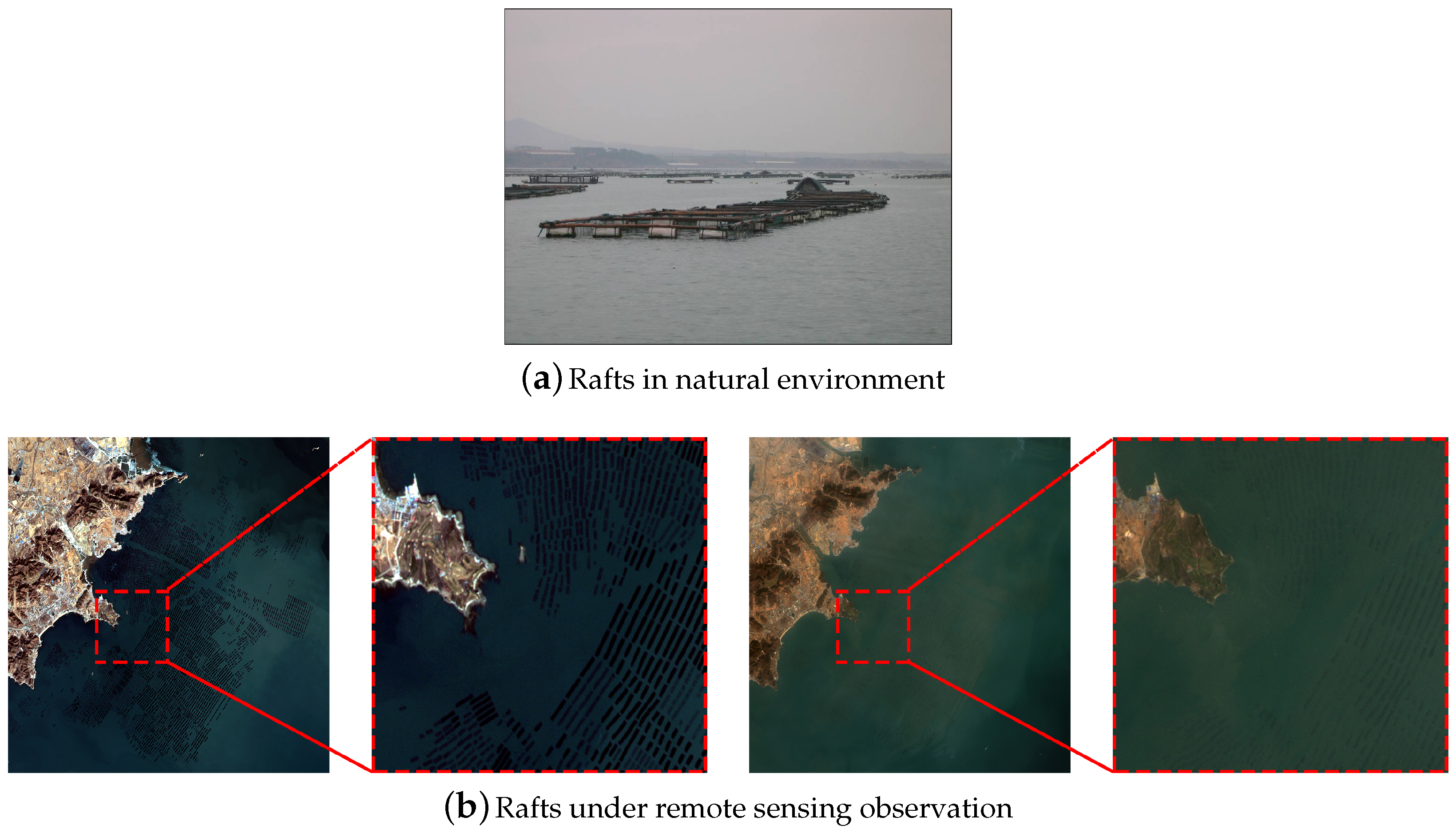
Raft-culture is a kind of aquaculture, where people use offshore waters to cultivate aquatic crops such as wakame, kelp and shellfish. The rafts are usually made up of floats and ropes, fixed to the seabed and neatly arranged on the water. With the fast development of optical remote sensing techniques, people nowadays are able to observe the states of rafts and control the growth of crops by remote sensing images. However, monitoring by manpower is extremely time-consuming and laborious. To obtain the accurate distribution and the area of these rafts, people have to manually label the large scale of the remote sensing image pixel by pixel. Usually, labeling one thousand square kilometers of sea area would take tens of hours of human work. Therefore, automatic raft-culture labeling by optical remote sensing is important for agricultural automation production and implementing effective management.
Rafts are usually small stripes with different lengths but the same width. The width of the strip is about 4–5 pixels (16-m spatial resolution).
Rafts are usually closely arranged near the coastline. The gap between adjacent stripes is about 2–5 pixels (16-m spatial resolution).
To tackle the raft-culture labeling problem, traditional methods start with the features of rafts and extract the shape, texture and color information. For optical remote sensing images, Liu et al. utilized the neighborhood statistics method by processing the blue band for remote sensing images [
1]. Wang et al. applied the region-line primitive association framework in raft-culture extraction [
2]. For SAR images, Fan et al. proposed joint sparse representation classification method based on the wavelet decomposition and gray-level co-occurrence matrix [
3]. Geng et al. combined the sparse representation classifier and the collaborative representation classifier with residual-based fusion strategy [
4]. However, the robustness of these methods cannot be guaranteed and their parameters have to be adjusted manually, especially when applied to complex ocean environments.
In recent years, Convolutional Neural Network (CNN) [
5] has played a very important role in the remote sensing field for image classification, detection, description and segmentation [
6,
7,
8,
9,
10,
11,
12], and it also has been widely used in many other fields [
13,
14,
15,
16]. CNN constructs multiple layers to learn high-level image features with better discrimination and robustness, as opposed to that in traditional methods [
17,
18,
19], where features have to be handcrafted. The rapid development of CNN gave birth to a new technology: Fully Convolutional Networks (FCN) [
20], which is specifically designed to predict a 2-D label map with the arbitrary-sized input image. FCN has greatly increased the processing flexibility and computational efficiency, and the image-to-image mapping process is naturally suitable for the pixel-wise image labeling tasks. In remote sensing image interpretation fields, such tasks include land structure segmentation, sea–land segmentation and others [
21,
22,
23]. However, raft labeling is different from the above labeling problems, where there is a huge difference between the semantic scales between them. In the former task, as rafts are always tiny and neatly arranged, one should mainly focus on some tiny structures and edges of the images, whereas in the latter task, one should pay more attention to the semantic information of a larger scale. This difference makes the traditional FCN based labeling method fail on this particular task. In fact, the key to tackling this problem is to explore and to take advantage of some important properties of an FCN model, e.g., invariance and equivariance, which is closely related to our problem.
Invariance is an important property for CNN and FCN, and it makes the network’s output stable to some changes of input of its scale and shape. Equivariance is another important property where the output of a network is sensitive to the input at the boundaries of different semantic classes. For a raft labeling task, both invariance and equivariance are needed. However, traditional FCN methods have strong invariance but lack equivariance. Thus, even the state of the art methods such as Deeplab [
24] cannot get clear and detailed labeling result of the rafts.
In this paper, we propose a new model called Homogeneous Convolutional Neural Network (HCN), which only consists of convolution and activation layers. In an HCN, all pooling layers are removed to retain all output details. The resolution of the output keeps the same as that of the input. As a result, all feature maps in an HCN share the same width and height to keep every details of an input image. In fact, in computer vision field, there are also some convolutional neural networks designed without pooling layers. Springenberg et al. replaced pooling layers by convolution layers with the same stride and the same kernel size to improve the network [
25]. He et al. proposed a residual network and also replaced the pooling layers by some residual blocks with strides [
26]. However, although pooling layers are removed in these methods, their output resolutions are still lower than the inputs, thus it is hard to obtain detailed raft labeling results.
Since rafts are usually located on the sea surface near land, it is crucial to remove land regions, which can mitigate the interference of some stripe-like objects. Note that, although one can easily generate the land mask by using geographical information and shore-line dataset, coastlines are frequently updated due to some human activations and it is hard for people to obtain an accurate and highly efficient coastline dataset. Therefore, in this paper, we further introduce a dual-scale version of HCN (DS-HCN), and this network can accomplish the sea–land segmentation task and the raft labeling task simultaneously in a semantic labeling fashion, i.e., label every pixel of the image into three classes, sea, land and rafts. The dual-scale structure of DS-HCN successfully addresses the huge scale gap between different classes, i.e., sea/land and rafts, and gives more accurate labeling results.
The contributions of our work are summarized as follows:
A new FCN based model, HCN, is proposed for the raft-culture labeling problem. HCN gives accurate and clear labeling results of tiny and densely arranged rafts with a noticeable performance improvement over the state of the art labeling methods.
We further propose a dual-scale version of HCN to tackle the sea–land segmentation and the rafts labeling in a uniform framework. Such approach gives further accuracy improvement of rafts recognition.
The rest of this paper is organized as follows. In
Section 2, we introduce Fully Convolutional Network and our proposed method in detail. In
Section 3, we further discuss our method based on some experimental results. Finally, conclusions can be found in
Section 4.
2. Methodology
In this section, we first give a brief review of the traditional FCN model and then give a detailed introduction for our proposed HCN and its dual-scale variant DS-HCN.
2.1. Fully Convolutional Network Framework
In general, the main calculations under the FCN framework include convolution, activation and pooling.
Convolution. A convolution layer is often made up of multiple kernels, which are used to separately convolute with the input data. This kind of layers aims at automatically extracting various local features from images, and these features can finally compose semantic information by layer stacking.
Activation. The non-linearity of a network is contributed by activation layers, and it ensures that the network is able to handle non-linear problems. Activation layers are usually attached to convolution layers with the element-wise operation, where the most popular activation functions are ReLU [
27] and its variants [
26,
28].
Pooling. A pooling layer can often be found after convolution and activation layers. This layer is designed to down-sample feature maps for speeding up the calculation, improving the invariance and the generalization ability of a network. Max-pooling is the most common operation to obtain results from each local region of the input.
FCN shares similar structural units to CNN, while their major difference is at the decision layer, where the fully connected layers in CNN are replaced by convolution layers with sized convolution kernel. Since convolution operation would not limit the input image size, FCN allows arbitrary-sized input image, which brings the concept of the receptive field.
The receptive field plays a key role in the FCN, and it limits the range of input pixels involved in the calculation, when predicting the semantic label for a pixel. Obviously, a small receptive field will make it difficult for a network to perceive global information. Generally, the receptive field is expanded by introducing convolution layers and pooling layers, so the classical fully convolution networks tend to use a deep structure with several pooling layers.
For a pixel-wise labeling task, a softmax loss is usually chosen as the loss function at the end of a network, which is equivalent to the pixel-wise accumulation of negative log-likelihood of the output class-probability.
2.2. Homogeneous Convolutional Network
Traditional semantic segmentation methods in computer vision field usually apply down-sampling operations to improve the invariance, and final full-sized outputs are usually enlarged by interpolation or deconvolution [
20,
24,
29,
30,
31]. Similar to a sampling problem in the signal processing field [
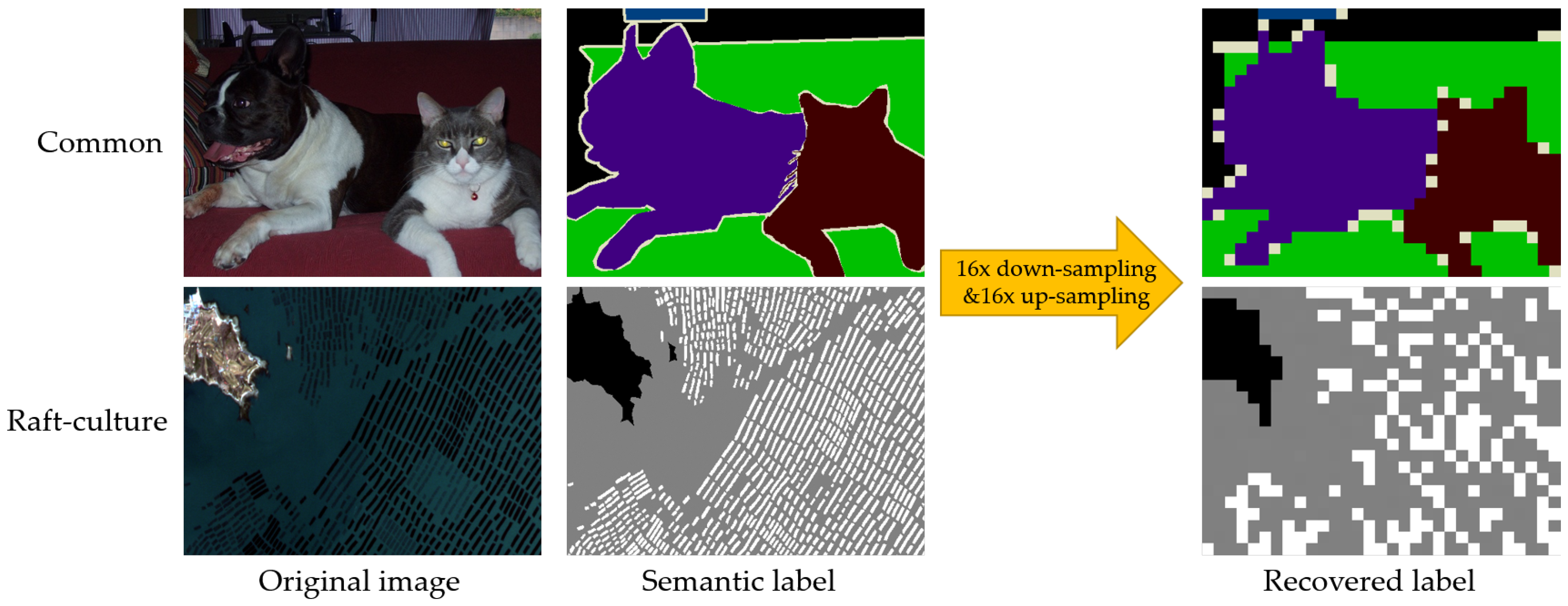
32,
33], the times of down-sampling has an upper limit for an FCN method to recover every detail of the input. For natural images, the foreground objects are usually large in size, which allows the neural networks to have some pooling layers or other similar structures to balance the equivariance and invariance. However, raft-culture remote sensing images contain rich semantic details. Thus, when applying multiple down-sampling operations, the original semantic information of those rafts will be difficult to recover, as shown in
Figure 2.
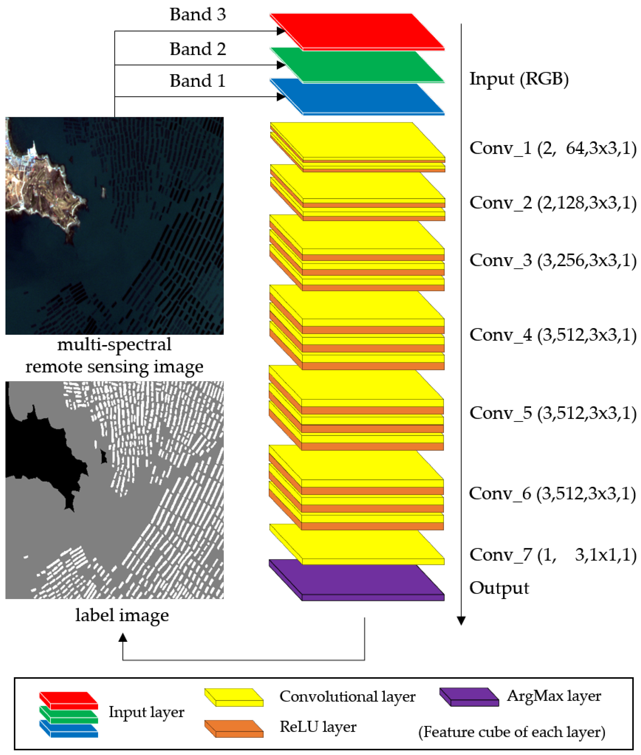
Based on the above analysis, we chose a high-performance 16-layer classification network (VGG-16 [
35]) as the backbone of our HCN model, and then all the pooling layers and fully connected layers are removed. As shown in
Figure 3, HCN contains only convolution and activation operations, which keeps the full resolution of all feature maps the same as the input image.
For a neural network, a deeper structure (more convolution layers) is helpful to further abstract features and improve the expression ability [
36], and a wider structure (more convolution filters) means that various features can be extracted. In the raft-culture labeling task, there are only three kinds of category required to recognize, so the depth is more important than the width. Therefore, we add two additional convolution layers to the end of the VGG-16, where the filter number is set to 512, half as much as that of VGG-16, for controlling the number of parameters.
As a comparison, the down-sampling times of Long’s FCN [
20] and DeepLab [
24], the classical semantic labeling methods, are 32 and 8, respectively, which are much larger than the width of rafts. Thus, the direct application of these networks in raft-culture would have difficulty obtaining accurate labeling results.
2.3. Dual-Scale HCN
Another difference between natural images and remote sensing images is about the scale. The objects in natural images are diverse, even those that are in the same category. In contrast, in remote sensing images, the intra-class objects are always in a similar size and shape, but the scales of inter-class objects are quite different, e.g., sea/land and rafts. Therefore, it is feasible to sacrifice the intra-class invariance introduced by pooling layers to get all detailed information.
However, a disadvantage of removing all pooling layers is the decrease of the receptive field. For example, the receptive field of the homogeneous convolutional network is only . In this case, there are some raft-like shapes in images miss-labeled as positive samples. Therefore, we further introduce an extra branch with a large receptive field, which is designed to integrate functions of the raft-culture distribution detection and the sea–land segmentation. That is, the improved HCN becomes a unified framework to tackle multiple tasks on different scales.
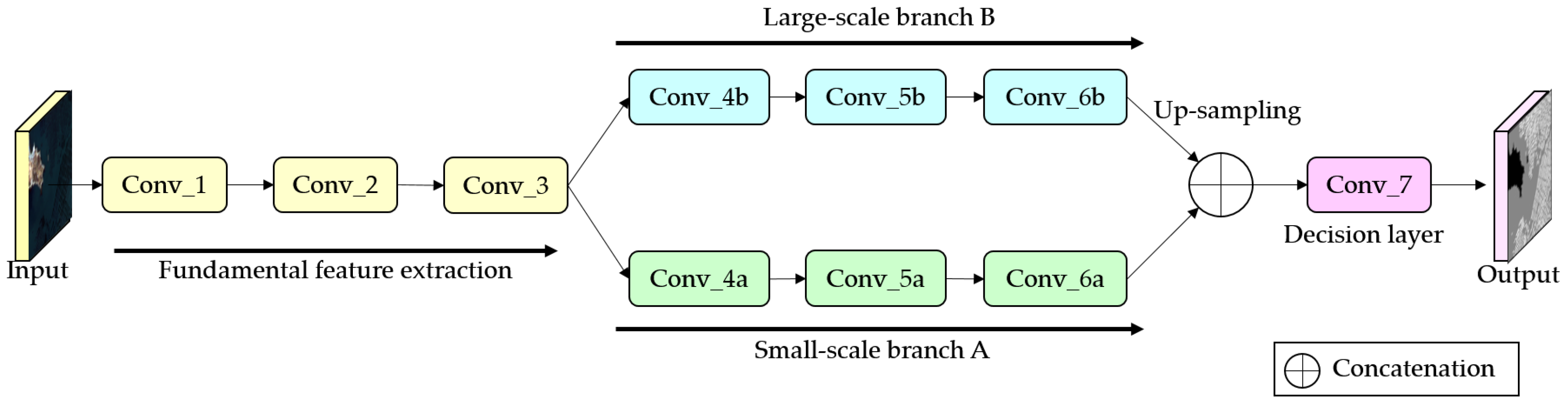
As shown in
Figure 4 and
Table 1, DS-HCN has two branches. Branch A is the same as the single-scale version with a small receptive field, as we have introduced in
Section 2.2. Branch B is improved from VGG-16 with some dilated convolutions [
24] for a larger receptive field, which could extract large-scale spatial information such as sea–land distribution and rafts distribution. Thus, when the features of the two branches are combined, the false-positives of Branch A will be suppressed by Branch B, and the features from Branch B can be regarded as a kind of prior information of the rafts’ distribution.
As for the structure of dual-scale version, the new branch includes three groups which, respectively, have 3, 3 and 1 convolution layers with 512 convolution kernels. Besides, for the first layers in Conv_4b and Conv_5b, the stride of these layers are set to 2 for enlarging the receptive field. Finally, outputs of two branches are resized to the same size and concatenated to a 1024-dimensional feature cube, and then the final output will be generated by Conv_7.
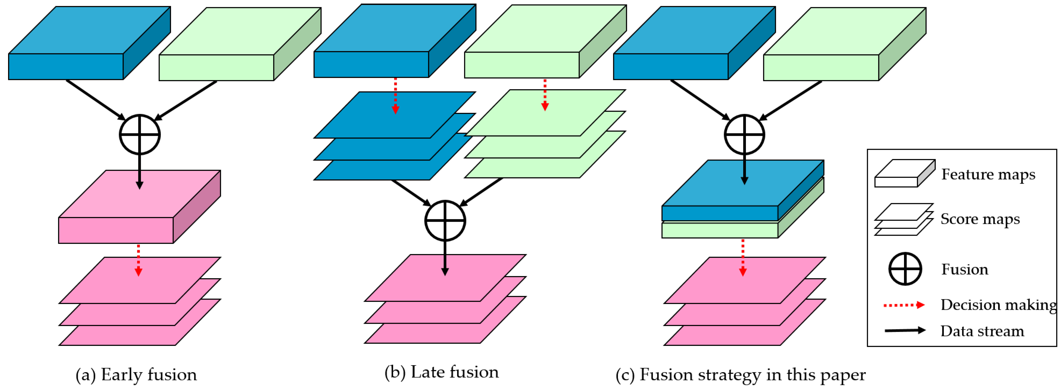
2.4. Fusion Strategy
For the fusion operation of different features in a convolutional neural network, some classical fusion strategies are early fusion and late fusion, as shown in
Figure 5.
Early fusion is feature-level, which refers to merging kinds of features into stronger ones. There are two classical early fusion methods: high-level and low-level fusion by skip connections [
37,
38] and multi-scale fusion by constructing feature pyramid [
20,
24,
39].
Late fusion is used in decision-level, which combines several decision results by voting, finding maximum, or counting mean value [
40,
41,
42,
43]. Generally, it takes multiple loss functions to build multiple multi-task optimization problems, and the final output consists of every weighted decision scores.
In this paper, we utilize the early fusion strategy to further improve the performance of our proposed network. By setting dual branches, we construct two different scales to extract texture information (small scale) and environmental information (large scale) for remote sensing images. As for the raft-culture labeling task, texture information refers to the edges of rafts, and environmental information means the regions of sea–land.
However, different from classical early fusion methods, the fusion strategy in DS-HCN is to concatenate dual-scale feature rather than adding them together. Suppose that
and
are the weight matrices and the bias vector of the decision layer,
and
represent the features extracted by each branch, and
means the concatenation of
and
, then the output sore map
can be split into two parts
and
which represent the decisions of Branch A and Branch B, respectively. Then, these three decisions have the following relations:
where
and
are the first and last part of
, respectively;
and
are the weighting coefficients; and the asterisk (*) represents the convolution operation.
DS-HCN has a good interpretability. As the above relations, this kind of fusion strategy is equivalent to the weighted mean (late fusion) of each branch’s decision result, but the weighted factors are learnable. That is, our method takes advantage of both fusion strategies. Therefore, it is easy to visualize the decision result of each branch.
3. Experiment, Results and Discussion
We designed three experiments to verify the effectiveness of our method. The first experiment was used to evaluate the performance of the classical adaptive threshold method (AT) [
1], a state-of-the-art semantic labeling method DeepLab [
24], HCN and its dual-scale version DS-HCN. The second experiment was designed to explore the effect of different scales on raft labeling. We further designed an experiment to parse and visualize the outputs of each branch of DS-HCN, which is helpful to analyze how the branches cooperate with each other in our task.
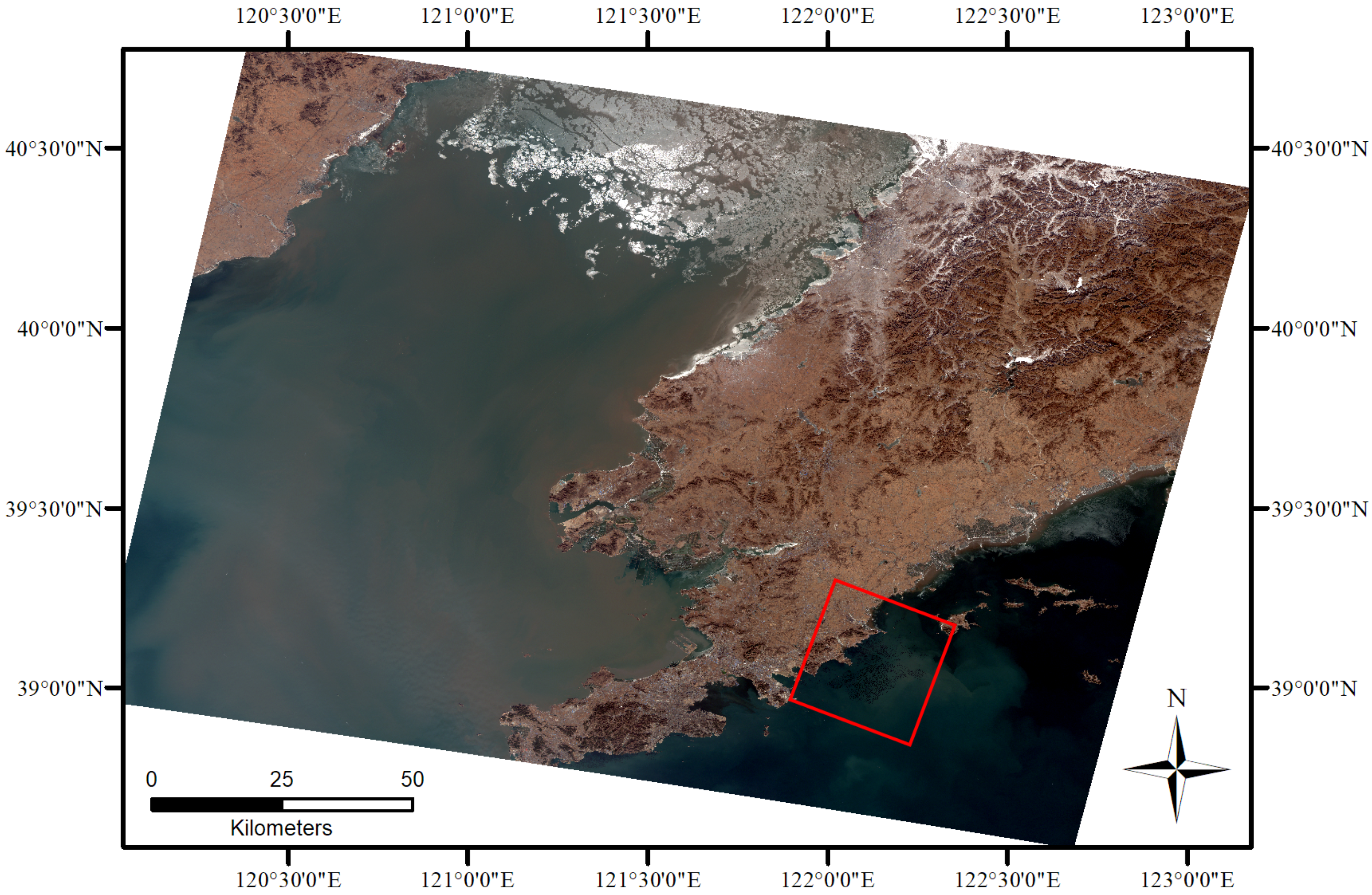
3.1. Dataset and Evaluation Criteria
A raft-culture dataset is built for experiments. Our dataset contained 56 remote sensing image slices and corresponding pixel-wise ground truth labels. We used 40 of them for training and the rest for testing. Images of our dataset were captured by the Gaofen-1 Wide field of view camera at different times with 16-m spatial resolution and the size of
pixels. The geographical location of the images is near Dalian, China, as shown in the red rectangle in
Figure 6. It should be noted that, since the original Gaofen-1 image (original Gaofen-1 images were provided by China Centre For Resources Satellite Data and Application (
http://www.cresda.com/)) is a 16-bit depth and 4-band image, all images were converted to 8-bit RGB images before being fed into the networks.
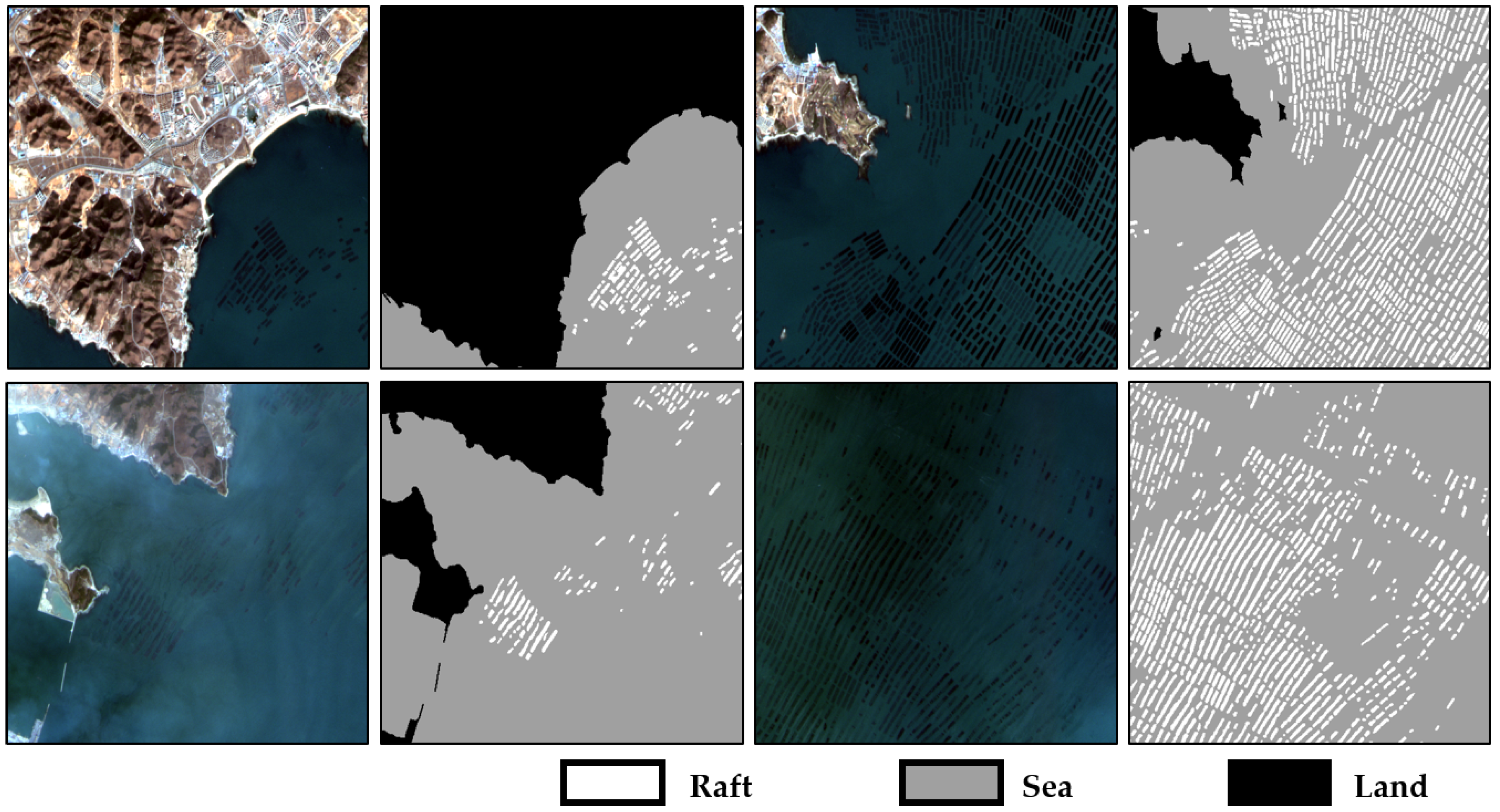
Figure 7 shows some examples and corresponding ground truth labels of our dataset.
The ground truth labels of our dataset contain three categories representing land, sea and raft, respectively.
In our experiments, we used softmax-loss and weighted-softmax-loss for pixel-wise computing the distance between outputs and labels. Our primary task was that the accuracy of rafts’ labeling is as high as possible, and the secondary task was to obtain a good result of sea–land segmentation.The formulas of softmax, softmax-loss and weighted-softmax-loss for a single pixel are shown as Equations (
2)–(
4).
where
and
are an output vector and the corresponding probability vector,
is the
k-th weight parameter and its value is inversely proportional to the pixel number of the corresponding category,
is the one-hot label,
L is the loss and
K is the number of categories. Furthermore, we used intersection over union (IOU) as our core evaluation criterion, which is defined as Equation (
5).
where
is the area ratio of overlap and union between pixel-wise labeling result (
) and ground truth (
). Similarly, precision (
P) and recall (
R) can be defined as:
3.2. Accuracy
In this experiment, we mainly verified the performance of the proposed method and choose HCN and DeepLab as comparisons. Each image of the training set was augmented by rotation, gamma transformation, contrast and saturation transformation for better generalizability. In addition, the three networks were initialized by pre-trained models. Particularly, we fine-tuned HCN by VGG-16 pre-trained on Imagenet, DeepLab by the provided model and DS-HCN by combining trained models of HCN and VGG-16. The training method is the stochastic gradient descent method with momentum and the hyper-parameters are set as follows: the learning rate is , the decay of learning rate is 0.9 per 5000 steps, the maximum number of iterations is 40,000, the momentum is 0.9 and the batch size is 8. Furthermore, due to the down-sampling process, it is hard for DeepLab to learn the details as rafts, so we used the weighted-softmax-loss when training DeepLab.
For further comparison, we adopt the adaptive threshold method (AT) as the baseline. There are three steps: (1) Convert test images to gray ones. (2) Orderly apply the adaptiveThreshold() and medianBlur() in OpenCV [
44] to process gray images. (3) Repeatedly adjust the parameters of those functions until achieving the best IOU. Finally, the optimal parameter settings are shown in
Table 2.
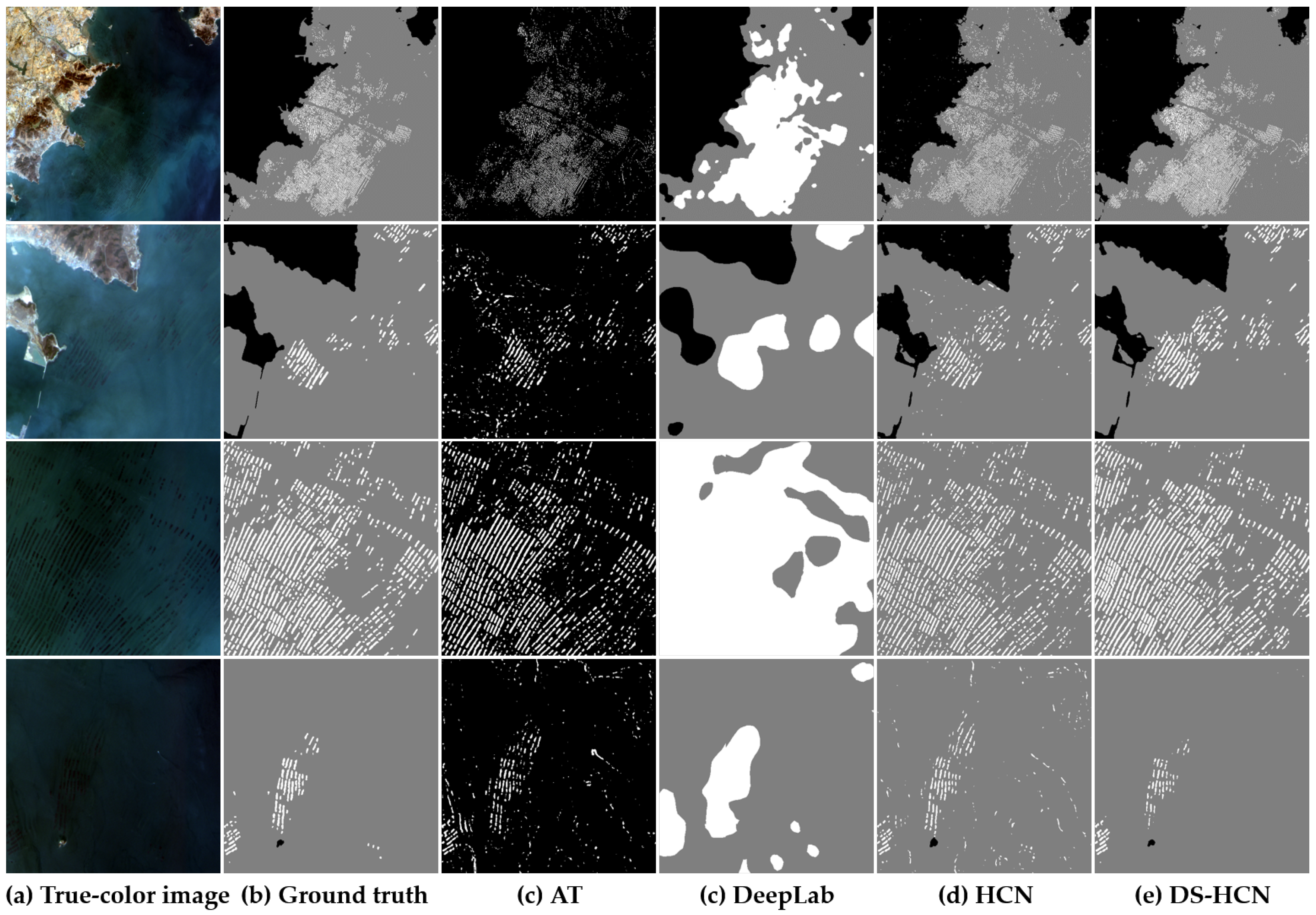
As shown in
Figure 8, because of the complex marine environment, the baseline method cannot fit all possible situations, so there are many errors in the binary results. As for deep learning methods, the robustness and automaticity are greatly improved, which is mainly because the neural network can learn and extract good features instead of manual ones. Nevertheless, based on the experimental results, HCN-based methods are superior to classical neural network (DeepLab) in rafts extracting. Generally, pooling layer is used to overcome tiny deformation by shrinking the size of feature maps, but it can also lead to a lower spatial resolution, and then the network will lose a lot of boundary information. Therefore, the results extracted by DeepLab are area-based, and then densely arranged rafts are treated as a whole. On the contrary, HCN has no pooling layer; each pixel of output can be directly mapped to input other than obtained by interpolation, so the boundary information of rafts can be kept as much as possible, which means HCN framework is suitable for the raft extraction task with remote sensing images.
Although HCN shows its good ability to extract rafts, there are still many false-positive errors in its results, and those error-pixels are located around the coastline and on the sea, where the places have complex texture. This phenomenon indicates that the basic HCN with a small receptive field overly focuses on small-scale features and ignores the large-scale information. Thus, DS-HCN combines a large receptive field to overcome this shortcoming and makes it possible to mine the association between multiple targets. Based on
Figure 8 and
Table 3, DS-HCN achieves the best performance and suppresses most of the false-positive errors by using prior information that rafts densely gather together and only exist on the sea.
As for the speed of extraction, DS-HCN can reach a million pixels every three seconds under NVIDIA Titan X Pascal by using deep the learning framework Caffe [
45]. In summary, to label a 2000 × 2000 remote sensing image including a whole raft-culture area only needs 12 seconds which is much faster than artificial labeling speed.
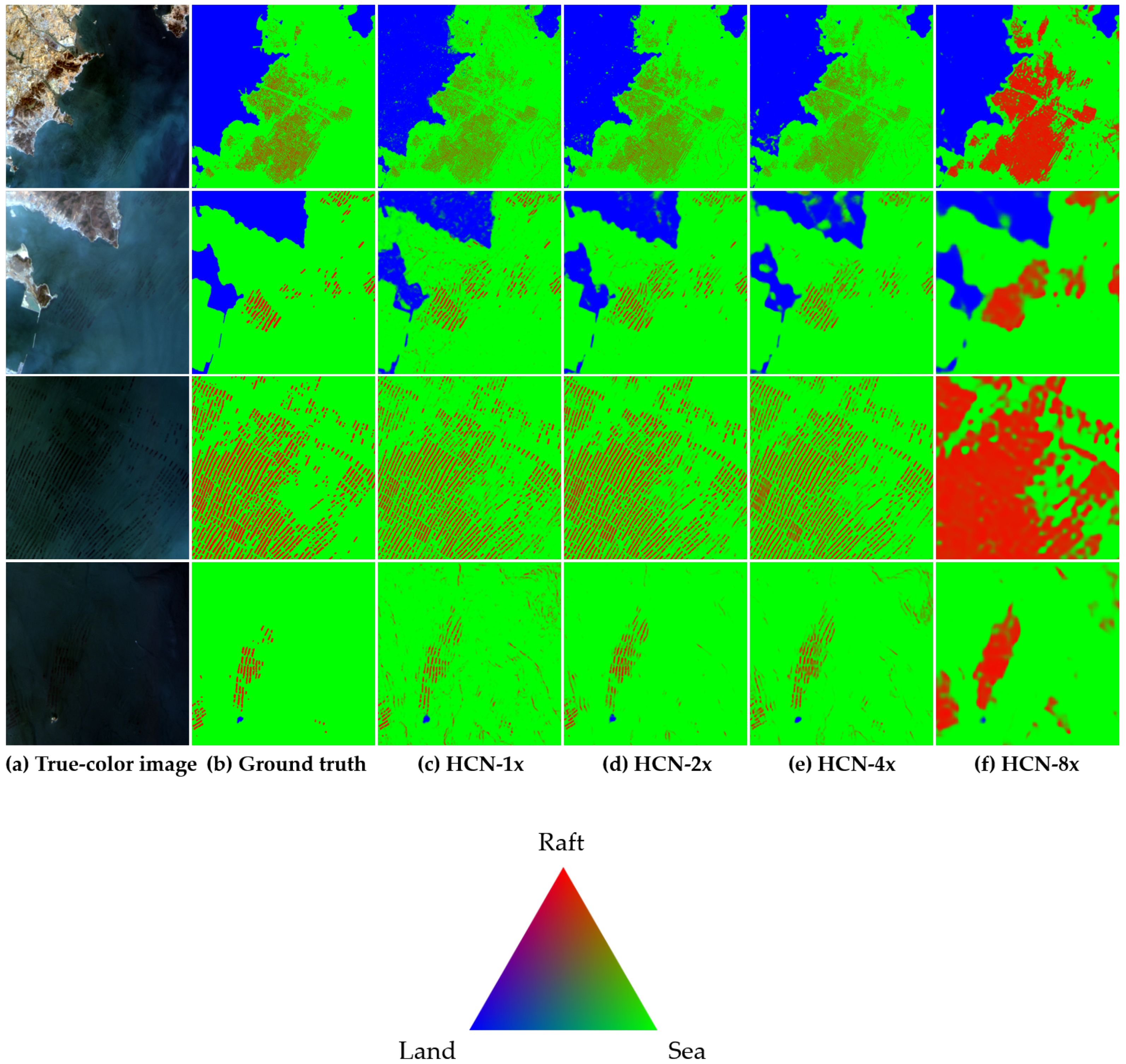
3.3. Scale Experiment
In this experiment, we aimed to study the effect of different scales on raft labeling. To achieve this goal, we added pooling layers at the end of the first few convolution groups in HCN, and the stride of each pooling layer was set to 2. By controlling the number of pooling layers, we can obtain four networks with different scales: 1× (original HCN), 2×, 4× and 8× (with weighted-softmax-loss), e.g., 8× represents that there are three pooling layers added to the back of Conv_1, Conv_2 and Conv_3, respectively. Then, we trained these four networks as the training strategy in the first experiment. Besides, we normalized the labeling results of these networks as the probability form (non-negative and sum-to-one) by employing soft-max function as Equation (
2). Since the probability vector
is three-dimensional, we further visualize the probability map in
Figure 9, of which color follows
and
. Finally, for each network, we present its precisions, recalls and IOUs of pixel-wise predicting results in
Table 4.
According to
Figure 9, as the down-sampling multiple increases, the loss of the small-scale information becomes more and more serious, but the large-scale information gradually plays an important role, so the corresponding probability maps become more and more blurred. This phenomenon is similar to the sampling theorem in the signal processing field, that is, the high-frequency information (small-scale semantic information) needs a high sampling frequency (few pooling layers) to guarantee that the original semantic information can be restored.
Since the interval and the width of most rafts are more than two pixels, the minimum period of the raft-related semantic signal can be considered to be greater than 4 pixels, which is exactly twice the sampling period of HCN-2×. That is, as long as the sampling period is less than that of HCN-2×, all the detailed information can be captured. However, the environmental information is also important and helpful for suppressing false-alarms, thus HCN achieves the best performance at the double down-sampling scale with a relatively large receptive field, as shown in
Table 4.
Based on this experiment, it can be found that the networks usually focus on their own scales, which means that the multi-branch structure can receive more information from different scales. Therefore, we chose the sharpest one and the smoothest one to structure the dual-scale neural network. Compared with HCN-2×, DS-HCN significantly improves the IOU of rafts with a 4.7% increase (
Table 3 and
Table 4).
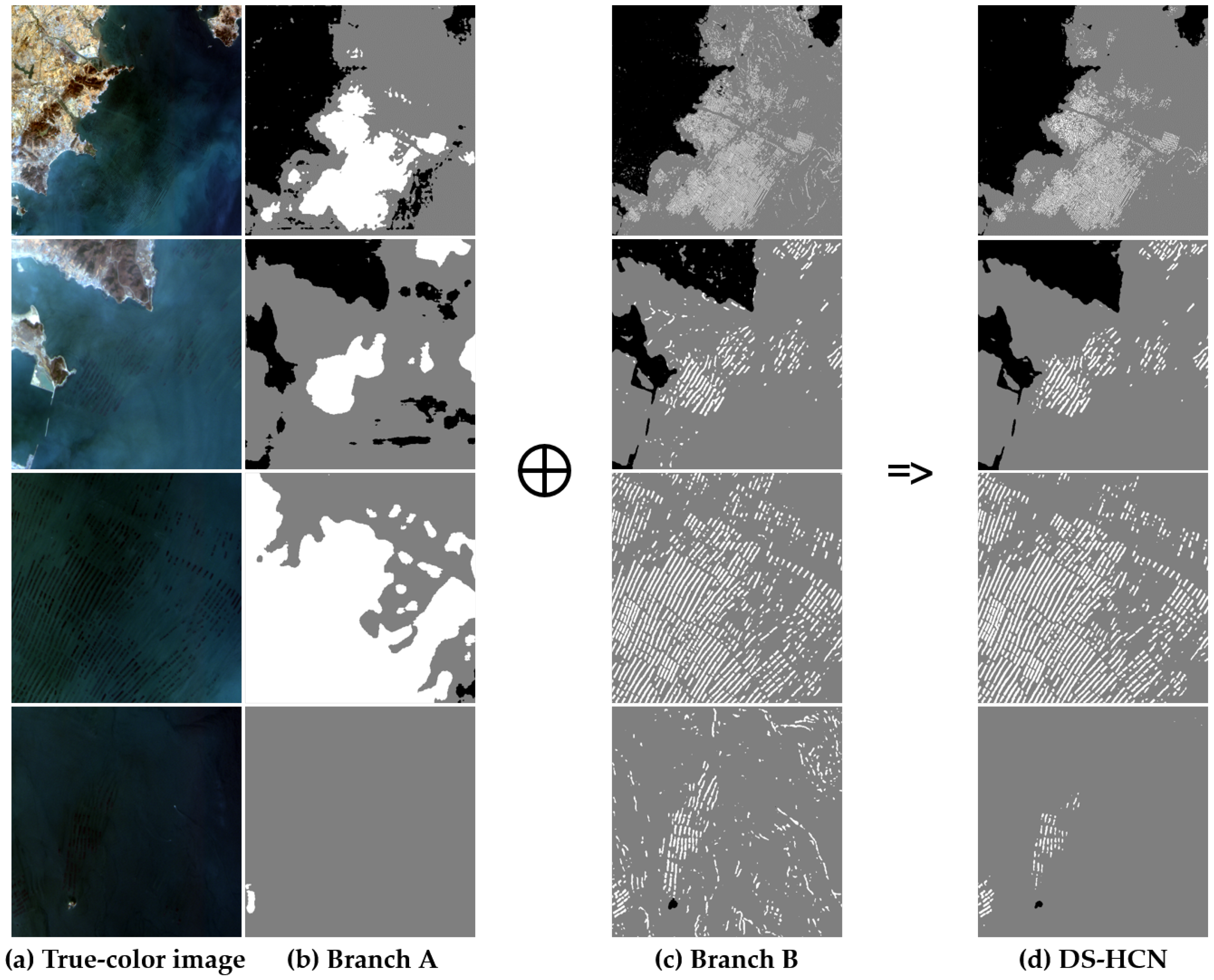
3.4. Interpretability Experiment
In this experiment, we tried to glimpse the internal working of our proposed method based on the first experiment. In detail, each branch in DS-HCN contributes to output, so we can split the final result by using each branch’s features. Based on Equation (
1), we set the output features of Branches A and B to
and
as
and
, respectively; split the convolution kernels in Conv_7 of DS-HCN to corresponding two parts
and
; and suppose that each branch has the same contribution, which means
. Then, we can get the following formulas in Equation (
8):
Finally, after sending the three score maps to the ArgMax layer, isolated decision maps are shown in
Figure 10.
It is worth mentioning that formulas in Equation (
8) are approximate calculations for two branches, so images in
Figure 10b,c are only sketches. Nonetheless, benefitting from the dual-scale structure, it can be found that the proposed network did successfully learn two different information scales, and the behaviors of the branches in our network are similar to the original ones. Besides, the fusion process of these dual branches can be found in
Figure 10.
Branch A, a small-scale HCN-like branch, contributes to the clear boundary for each raft, as shown in the third column in
Figure 10. However, in a complexly practical situation, many other objectives would be identified by mistake. To overcome this weakness, Branch B is used to contribute to the general distribution of each category. Further, when combining the two contributions, spatial relations will become apparent. For instance, if a pixel is considered as raft by Branch A but sea by Branch B, then this pixel will be confirmed as the sea with high probability in the end, since this pixel is out of rafts’ range, as shown in the fourth row of
Figure 10. Therefore, by integrating dual branches, it makes our method possible to learn some prior information about spatial relations, and then each branch will have its specifically practical meaning.
Based on this experiment, our proposed method shows good interpretability, and the decisions of each branch can be easily visualized. This is very useful to analyze the behavior of the neural network and further improve it. In addition, benefiting from the fusion strategy used in this paper, the neural network can automatically learn the fusion weights of different scales according to the training samples to obtain the end-to-end labeling results under a uniform framework.
4. Conclusions
In this paper, we propose the homogeneous convolutional network (HCN) to solve the problem of raft-culture remote sensing image labeling. This network consists of 17 convolution layers and corresponding ReLU layers, which has the largest spatial resolution and can distinguish tiny rafts in images. Furthermore, we introduce dual-scale version (DS-HCN), and it contains two branches with different receptive fields. The bigger one aims to extract the distribution of each category, and the smaller one only aims to catch every detail. Based on the three experiments, we can obtain the following three conclusions: (1) The network without down-sampling can capture the very small rafts, and the dual-scale structure will contribute to suppressing the false-positive errors. This structure may also be used in labeling other small objects, e.g., ships, buildings and roads, especially when using the relatively low-resolution remote sensing images. (2) Different scales represent different semantic information, and small objects need a high-resolution network to be distinguished, such as HCN. (3) The fusion strategy (concatenation) in this paper can help a multi-scale network more easily visualize its decisions from different scale features. In summary, our DS-HCN has high precision and good interpretability, and it is suitable to solve the raft-culture labeling problem.


