Article

High-Resolution Remote Sensing Image Classification Method Based on Convolutional Neural Network and Restricted Conditional Random Field

1
School of Computer & Information Technology, Changchun Institute of Technology, Changchun 130012, China
2
The Key Laboratory of Changbai Mountain Historical Culture and VR Technology Reconfiguration, Changchun 130012, China
*
Author to whom correspondence should be addressed.
Remote Sens. 2018, 10(6), 920; https://doi.org/10.3390/rs10060920
Submission received: 18 April 2018 / Revised: 25 May 2018 / Accepted: 8 June 2018 / Published: 10 June 2018
(This article belongs to the Special Issue Recent Advances in Neural Networks for Remote Sensing)

Abstract

:
Convolutional neural networks (CNNs) can adapt to more complex data, extract deeper characteristics from images, and achieve higher classification accuracy in remote sensing image scene classification and object detection compared to traditional shallow-model methods. However, directly applying common-structure CNNs to pixel-based remote sensing image classification will lead to boundary or outline distortions of the land cover and consumes enormous computation time in the image classification stage. To solve this problem, we propose a high-resolution remote sensing image classification method based on CNN and the restricted conditional random field algorithm (CNN-RCRF). CNN-RCRF adopts CNN superpixel classification instead of pixel-based classification and uses the restricted conditional random field algorithm (RCRF) to refine the superpixel result image into a pixel-based result. The proposed method not only takes advantage of the classification ability of CNNs but can also avoid boundary or outline distortions of the land cover and greatly reduce computation time in classifying images. The effectiveness of the proposed method is tested with two high-resolution remote sensing images, and the experimental results show that the CNN-RCRF outperforms the existing traditional methods in terms of overall accuracy, and CNN-RCRF’s computation time is much less than that of traditional pixel-based deep-model methods.

Graphical Abstract

1. Introduction

With the rapid development of remote sensing technology, a large volume of high-resolution remote sensing images is now available. Using classification algorithms, land cover information can be extracted automatically from remote sensing images, allowing the massive amounts of remote sensing data already obtained from satellites to be fully utilized. In recent years, many algorithms have been introduced in the field of high-resolution image classification [1].
High-resolution remote sensing images contain abundant detailed land cover information, which can lead to considerable internal variability in a land cover category, resulting in low accuracy classification images when utilizing classification algorithms if they rely on only the band values of pixels [2]. To improve the results, algorithms should consider a pixel’s neighborhood as the context to discover the deeper characteristics of land cover from images [3]. When using classification trees, support vector machines (SVMs) and other traditional shallow classification models, object-oriented segmentation techniques, which can obtain relatively homogeneous areas and reduce the classification difficulty, are usually adopted [4]. However, segmentation algorithms typically rely on several pre-determined parameters. Because of the different scales involved in the different land covers in an image, these algorithms might result in both over- and under-segmentation within the same image [5]. This problem can be partially solved by introducing multi-scale technology such as hierarchical selection or supervised evaluation selection [6]; however, in these methods, multiple iterations of segmentation, evaluation, and parameter selection must be executed in subsequent steps, thereby further increasing the difficulty of model implementation and utilization. Meanwhile, along with improvement of the image resolution, single segmentation can hardly represent the characteristics of land cover category due to internal variability. Considering all the above limitations, it is imperative to introduce new technologies for classifying high-resolution remote sensing images.
In recent years, deep learning technology has achieved considerable success in such fields as signal processing, image identification, speech identification, and Go board position evaluation [7,8,9,10]. In the field of remote image processing, auto-encoders (AEs) and convolutional neural networks (CNNs) are the main focuses. AEs can reconstruct input data via encoding and decoding processes and obtain more optimized feature expressions, and the ability of an algorithm to filter noise from signals and identify objects in the image can be significantly improved through AE processing [11,12,13]. By integrating the spectral-spatial information of hyperspectral images, features with greater classification value can be constructed to improve classification accuracy [14]. The pan-sharpening method for remote sensing images is realized by an AE and achieves better results [15]. The features are extracted using the AE and the image classification quality is improved [16,17,18,19]. The hyperspectral data can be projected to a higher dimension using the AE to improve data separability, or attributes can be reconstructed and reduced to improve the classification quality [20,21]. An AE-based classification framework was created for land cover mapping over Africa [22]. A fuzzy AE is used to conduct cloud detection from ETM+ images [23]. For CNNs, convolutional layers and max-pooling layers are adopted to strengthen the image classification ability. CNNs can achieve favorable classification results, especially in the fields of object detection and scenario classification. Vehicles can be detected from remote sensing images using CNNs. The target recognition accuracy has been enhanced in SAR images by improving the CNN training method [24]. A pre-trained CNN from ImageNet was used to conduct object recognition [25], and a CNN was used to extract road networks [26]. The region-based CNN was improved to increase the precision of detecting geospatial objects [27]. The rotation-invariant characteristics of a CNN were enhanced by improving the objective function [28]. For scenario classification from remote sensing images, experimental results show that CNNs achieve higher classification accuracies compared to the bag of visual words (BOVW) and other traditional algorithms [29]. A pre-trained neural network extracts spatial attributes and can achieve higher accuracy than traditional feature representation algorithms [30]. CNNs describe multi-scale spatial patterns and improve the BOVW algorithm’s classification accuracy [31].
In the common CNN structure, the input is a feature map set and the output is a category label. Directly applying this structure to pixel-based remote sensing image classification will lead to boundary and outline distortions of the land covers in the result image [32]. To overcome this drawback of CNNs, three types of CNN-based strategies exist for performing pixel-based image classification. (1) The pixel-based classification can be realized by transforming the CNN input or output. For example, a central point enhancement layer can be introduced to weaken the translational invariance characteristics of the CNN to achieve pixel-based classification [32]. Integrating CNN output results and MLP output results can also improve the classification accuracy of the land cover boundary [33]. Nevertheless, algorithms of this type have a typical weakness: during classification, for every pixel in the image, an input feature map (or image patch) must be constructed and classified. When the image is large (e.g., a 6000 × 6000 image involves reading and classifying 36,000,000 image patches), this requirement constitutes a serious computational burden, causing the classification speed to be very slow. (2) Pixel-based segmentation can be realized by introducing fully convolutional networks (FCNs) into the CNN as a deconvolution output layer [3,34]. However, this type of algorithms requires a large amount of training data (e.g., training data obtained from many images) to train the neural network, and the model training stage requires multiple days or even weeks, even on a high-performance computer [35,36]. (3) The CNN first classifies the entire image to obtain rough superpixel classification results; then, it semantically segments the superpixel image using conditional random fields (CRFs) and refines the results into pixel-based classifications [37]. Land covers in remote sensing images have many categories and have different sizes. Different categories that have similar spatial band values will lead to excessive expansion or shrinking of partial land covers during the CRF segmentation process. Therefore, CRF segmentation is seldom utilized in the remote sensing classification field.
The motivation of this paper is to fully utilize the CNN’s classification ability, avoiding traditional CNN drawbacks of boundary or outline distortions of land cover, reducing computational time, and achieving the goal of realizing “reasonable training sample set size- > acceptable model training time- > acceptable entire image classification time- > higher classification accuracy” in high-resolution remote sensing image classification. This paper proposes a high-resolution remote sensing image classification method based on CNN and the restricted conditional random field algorithm (CNN-RCRF). CNN-RCRF adopts CNN superpixel classification instead of pixel-based classification and uses the restricted conditional random field algorithm (RCRF) to refine the superpixel result image into a pixel-based result. The proposed method not only takes advantage of the classification ability of CNNs but can also avoid boundary or outline distortions of the land cover and greatly reduce computation time in classifying images. The effectiveness of the proposed method is tested with two high-resolution remote sensing images, and the experimental results show that the CNN-RCRF outperforms the existing traditional methods in terms of overall accuracy, and CNN-RCRF’s computation time is much less than that of traditional pixel-based deep-model methods.

2. Methods

2.1. CNN and Image Classification

A convolutional neural network (CNN) is a multi-layer neural network different from general neural networks, CNN introduces convolutional layers and subsampling layers into its structure. Via the kernel, the convolutional layer performs a convolution calculation of the feature map input by the previous layer. Then, the transmission function can be calculated to obtain the output feature map. The formula for calculating the output feature map can be written as follows:
ξ j l = f ( i T ξ i l 1 × k i j l + b j l ) ,
where f is the transmission function, l corresponds to the current layer, ξ j l denotes the jth output feature map at the lth layer, T denotes all the input feature maps, k i j l corresponds to the weights of the kernels of the ith input feature map, and b j l is the bias of layer l [32]. The subsampling layer can realize the down-sampling of the input feature map, and the output feature map is smaller than the input feature map. The formula for calculating the output feature map can be written as follows:
ξ j l = f ( δ j l d o w n ( ξ j l 1 ) + b j l ) ,
where down is a down-sampling function that returns the maximum or minimum value within an n × n block (the maximum value is currently more widely used). A layer that uses the maximum value as a down-sampling function is called a max-pooling layer, and δ j l is the multiplier deviation of the jth feature map at the lth layer [38].
The CNN input is a feature map set (or an image patch). The CNN first uses multiple groups of convolutional layers and max-pooling layers to extract critical characteristics and reduce the number of neurons. Next, the feature maps are converted into a one-dimensional vector. Finally, a multi-layer fully connected neural network is used to determine the CNN output, which is a category label. This structure can effectively perform scene classification and land object detection. When this structure is used for pixel-based remote sensing image classification, if the category label is directly adopted as the category label for all pixels from the input feature map set, superpixel classification results will be obtained; this reduces the resolution of the original image [37]. If each pixel from the image is considered as a center point, and each center point and all its neighboring pixels are used to construct the feature map set, then the CNN determines the pixel’s category label based on this feature map set, which leads to boundary and outline distortions of the land covers in the result image [32]. Therefore, accurate pixel-based remote sensing image classification results are difficult to obtain via a CNN with a traditional structure.

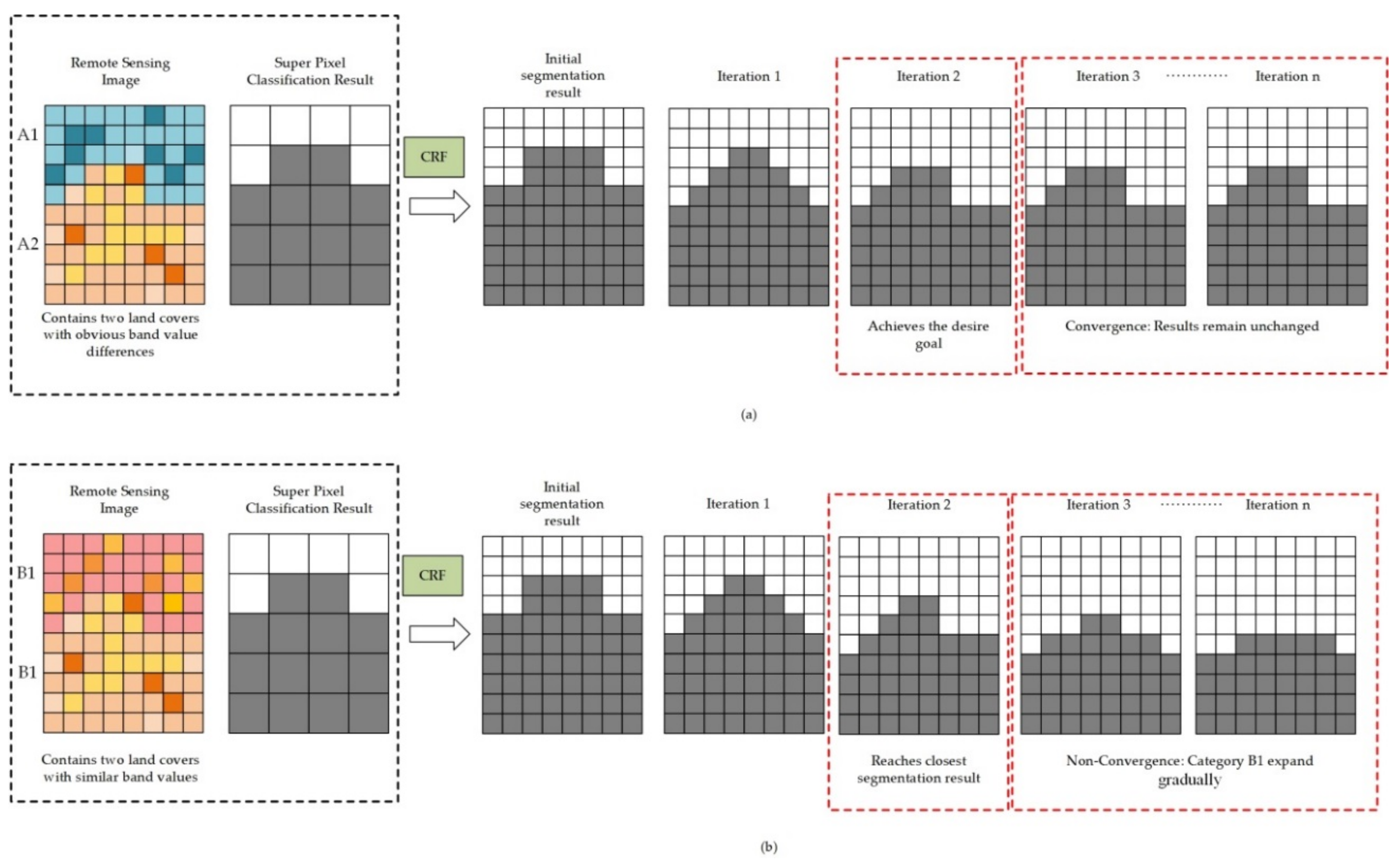
2.2. Fully Connected CRF

In the field of object identification, CRF is a classical segmentation method that can segment rough superpixel classification results into pixel-based classification results [39]. Consider a remote sensing image that contains N pixels and a random field I with random variables {I1, I2,…, IN}, where Ii is the vector constituted by the spatial-feature values of pixel i. Suppose another random field X with random variables {x1, x2,…, xN} exists, where xi is the category label of pixel i, whose value is a set of labels L = {l1, l2,…, lk}. A conditional random field (I,X) can be defined as follows:
P ( X | I ) = 1 Z ( I ) exp ( c C g log ( X C | I ) ) ,
where Z(I) is a normalizing factor that guarantees that the distribution sums to one:
Z ( I ) = X exp ( c C g log ( X C | I ) ) ,
where g = (ν,ε) is a graph on X, c is a clique in a set of cliques Cg in g induces a potential φc [40]. In each CRF iteration, the mutual interaction between pixels is calculated using the energy function [41]. The superpixel classification results obtained by the CNN are usually processed using the fully connected CRF. The fully connected CRF energy function can be expressed as follows:
E ( x ) = i θ i ( x i ) + i j θ i j ( x i , x j ) ,
where the unary potential θ i ( x i ) = log P ( x i ) and P ( x i ) represents the probability of pixel i belonging to the category label. The pairwise potential θ i j ( x i , x j ) can be written as follows:
θ i j ( x i , x j ) = μ ( x i , x j ) K i j ,
If xixj, then μ ( x i , x j ) = 1; otherwise, μ ( x i , x j ) = 0. The formula for Kij can be expressed as follows:
K i j = ω 1 exp ( p i p j 2 2 σ α 2 I i I j 2 2 σ β 2 ) + ω 2 exp ( p i p j 2 2 σ γ 2 ) ,
where pi and pj correspond to the positions of pixel i and pixel j, respectively. The first part of the formula describes the degree to which adjacent pixels with similar band values belong to the same category. Here, σа and σβ are used to control the weights of the position and the band value. The second part of the formula is used to eliminate relatively isolated areas in the image. Through the JointBoost algorithm, the values of ω1, σа, σβ, ω2 and σγ can be obtained from the image [42]. Using CRFs, the pixels affect one another through their energies, their category labels may change during iteration, and the rough superpixel results can be segmented into pixel-based classification results. The process of obtaining the pixel-based segmentation result via CRF is shown in Figure 1:
As shown in Figure 1a, in an ideal situation, the remote sensing image contains two land cover areas, A1 and A2 with obvious band value differences. In the segmentation process, CRF takes the super-pixel result as the initial segmentation result. According to the value of the image pixel bands and the category of neighborhood pixels, CRF using formula (3) is used to iteratively modify the category of each pixel in the segmentation result. This iterative process achieves the desired goal in the second iteration. Because there is an obvious difference between A1 and A2, the segmentation result is no longer changed during subsequent iterations; thus, convergence results are obtained. In this situation, CRF achieves good segmentation results easily. However, the spatial band values of adjacent land covers might be approximately equal, thereby making it difficult to confirm the boundary between them. Moreover, the areas of different land covers might differ greatly, or a land cover that belongs to a certain category might be too small or too large compared with other land covers. An example is shown in Figure 1b, in which the remote sensing image contains relatively similar categories B1 and B2. During the CRF iteration process, the second iteration reaches the closest segmentation result. Unfortunately, because the two categories are similar, in the subsequent iterative process, category B1 may expand gradually, causing the pixels at the boundary to be misclassified. In this situation, the number of iterations of the CRF should be assigned a suitable value, which is a challenge in the traditional CRF process (resulting in non-convergence). When the number of CRF iterations is inadequate, the obtained results will be too rough to obtain the entire image pixel-based classification results. In contrast, when the number of CRF iterations is too large, certain land covers might be excessively expanded, while others might be excessively reduced, thereby leading to a decrease in the classification accuracy. Therefore, when using a CRF segment method on remote sensing images, it is imperative to develop a new mechanism that resolves all the above problems of the traditional fully connected CRF.

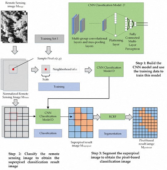
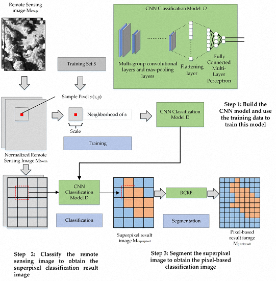
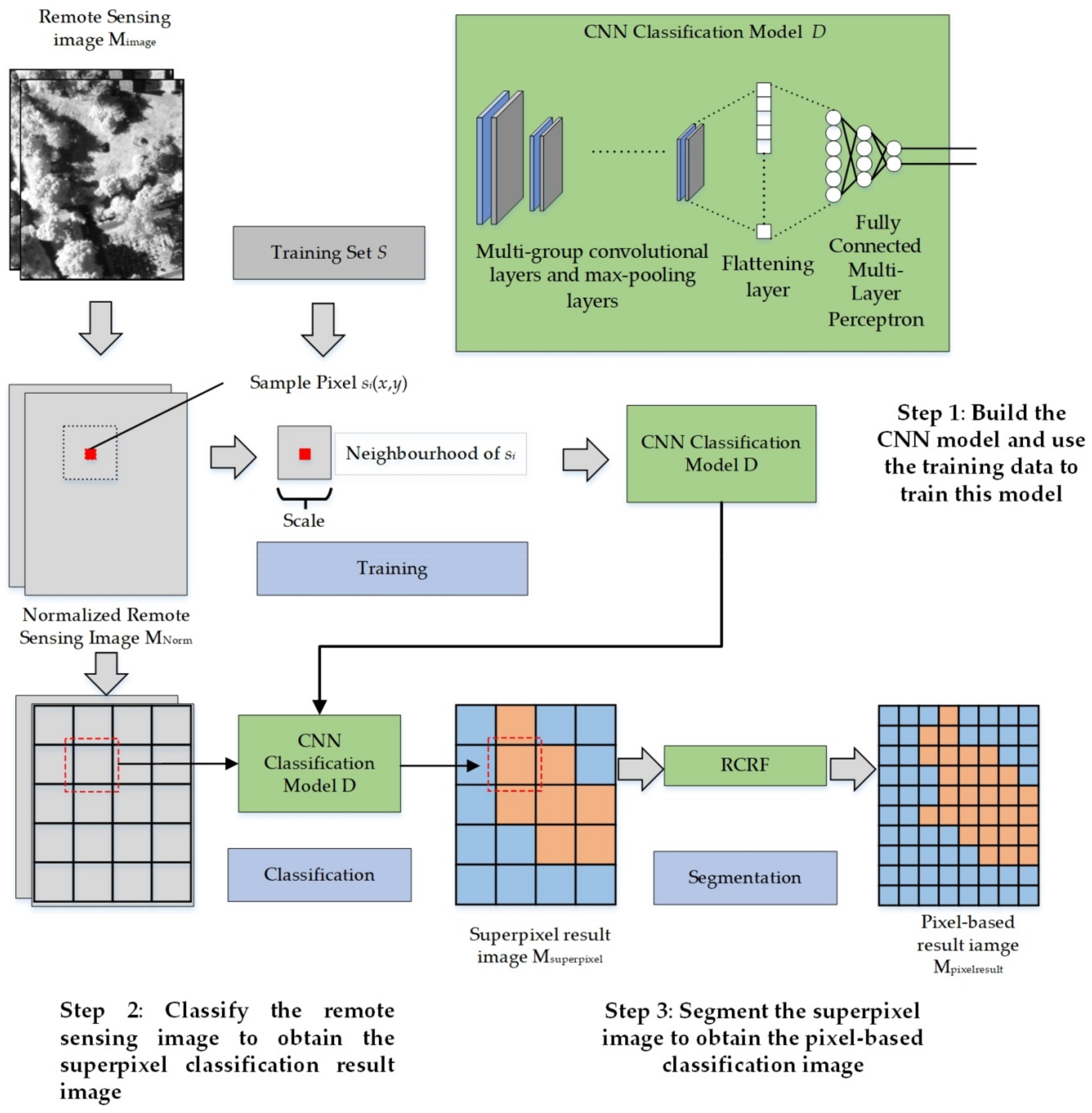
2.3. High-Resolution Remote Sensing Image Classification Method Based on Convolutional Neural Network and Restricted Conditional Random Field

As mentioned above, when a CNN with a traditional structure is directly used for pixel-based classification, boundary and outline distortions might occur, and when employing a CRF for remote sensing image segmentation, certain land covers might be excessively expanded or reduced. To address these limitations, this paper proposes a high-resolution remote sensing image classification method based on the convolutional neural network and restricted conditional random fields (CNN-RCRF). Figure 2 shows the process of the CNN-RCRF.
As shown in Figure 2, the CNN-RCRF involves three main steps.
Step 1: Build the CNN model and use the training data to train this model
Every spatial band of remote sensing image Mimage to be classified is normalized to the interval [0,1] to construct a normalized remote sensing image MNorm. Then, the CNN model D is created. The detailed information of this CNN model is shown in Table 1:
As shown in Table 1, this model contains the following components.
(1) Multi-group convolutional layers and max-pooling layers: The convolutional layer adopts ReLu as the transmission function. The scale of the convolutional kernel is 3 × 3, and convolution processing adopts the “padding = same” method, which ensures that the size of the feature map remains the same after convolutional processing. The max-pooling layer adopts 2 × 2 as the down-sampling size. The group number of convolutional layers and max-pooling layers can be written as the following:
N g r o u p n u m = { 1 , R o u n d ( log 2 ( S c a l e S c a l e target ) ) , S c a l e S c a l e t arg e t < 2 S c a l e S c a l e t arg e t 2 ,
where Scale is the input feature map size, and Scaletarget is the minimum target size after multi-group convolutional layer and max-pooling layer processing. Through Ngroupnum group convolutional layers and max-pooling layers input feature map size can be reduced and deeper representative characteristics can be extracted.
(2) Flattening layer: This layer converts the feature maps into a one-dimensional neural structure to improve the convenience of decision making.
(3) Fully Connected Multi-Layer Perceptron (MLP): The MLP is composed of three layers. An input layer connects to the previous flattening layer; the input and middle layer both adopt ReLu as the transmission function; and the output layer adopts softmax as the transmission function.
After creating the CNN model D, a sample set S = {s1, s2, s3,…,sN} containing N samples is introduced. Every sample si consists of the sample position (x, y) on the image and the corresponding category label L. Each sample at (x, y) and the surrounding square area with size Scale cuts an image patch from MNorm. The samples’ corresponding image patches and category labels are used as training data and input to D to obtain the trained CNN model D which can then determine a new image patch’s category label.
Step 2: Classify the remote sensing image to obtain the superpixel classification result image
As shown in Figure 2, the feature map size Scale is used to split MNorm into image patches. If the feature map exceeds the boundary of MNorm, boundary pixel mirroring is conducted to fill the image patch to ensure that the image patch’s size is equal to Scale. Every image patch is classified by the CNN model D to obtain a category label. In the result image Msuperpixel, this category label is assigned to every pixel in the area of the corresponding image patch. Msuperpixel is the superpixel image, and its resolution is lower than that of the original image. Therefore, follow-up processing must be performed to obtain a pixel-based classification result image.
Step 3: Segment the superpixel image to obtain the pixel-based classification image
In Step 3, Msuperpixel, which was obtained through Step 2, is segmented to obtain the pixel-based result Mpixelresult. To obtain a good segmentation result and avoid land cover expansion or reduction problems caused by inadequate or excessive iterations of traditional CRF, this paper proposes an algorithm (described as Algorithm 1) that controls the number of CRF iterations based on the training samples:
Algorithm 1 Sample-Based Iteration Control Algorithm (SBIC)
Input: Remote sensing image Mimage, superpixel image Mtarget with two categories (“target” and “background”), sample set Sobject with two categories (“target” and “background”), maximum number of iterations Nmax
Output: Result image Mresult after segmentation
Begin
ResultArray[Nmax] = based on Mtarget and Mimage, conduct Equation (3) in Nmax iterations, save each iteration’s result into ResultArray;
previousAccuracy = 0;
pos = 0;
for i in 1:Nmax {
  accuracy = Use Sobject to calculate the classification accuracy in ResultArray[i];
  if previousAccuracy ≤ accuracy {
   previousAccuracy = accuracy;
   pos = i;
  else
   break;
  }
}
Mresult = ResultArray[pos];
 return Mresult;
End
Based on this algorithm, every sample in Sobject contains both a sample position and category label. Calculating the number of samples that are correctly classified can help obtain the classification accuracy of Mresult. The SBIC algorithm can be used to conduct continuous segmentation of Mtarget, which is composed of two categories (target and background), to obtain the pixel-based result. In each iteration of the SBIC, Mtarget is segmented by the fully connected CRF in one iteration. Then, Sobject is used to test the classification accuracy. If the classification accuracy remains the same or has improved after the iteration, excessive expansion or shrinking has not occurred; consequently, the fully connected CRF can proceed with the next iteration. In contrast, if the classification accuracy has been impaired after an iteration, iteration should be halted, and the result of the previous iteration should be adopted as the final result. The SBIC algorithm uses the test samples to limit the number of fully connected CRF iterations. Based on the SBIC, this paper further proposes the RCRF algorithm. The process of the RCRF algorithm is shown in Figure 3.
As shown in Figure 3, the RCRF algorithm can be described as Algorithm 2.
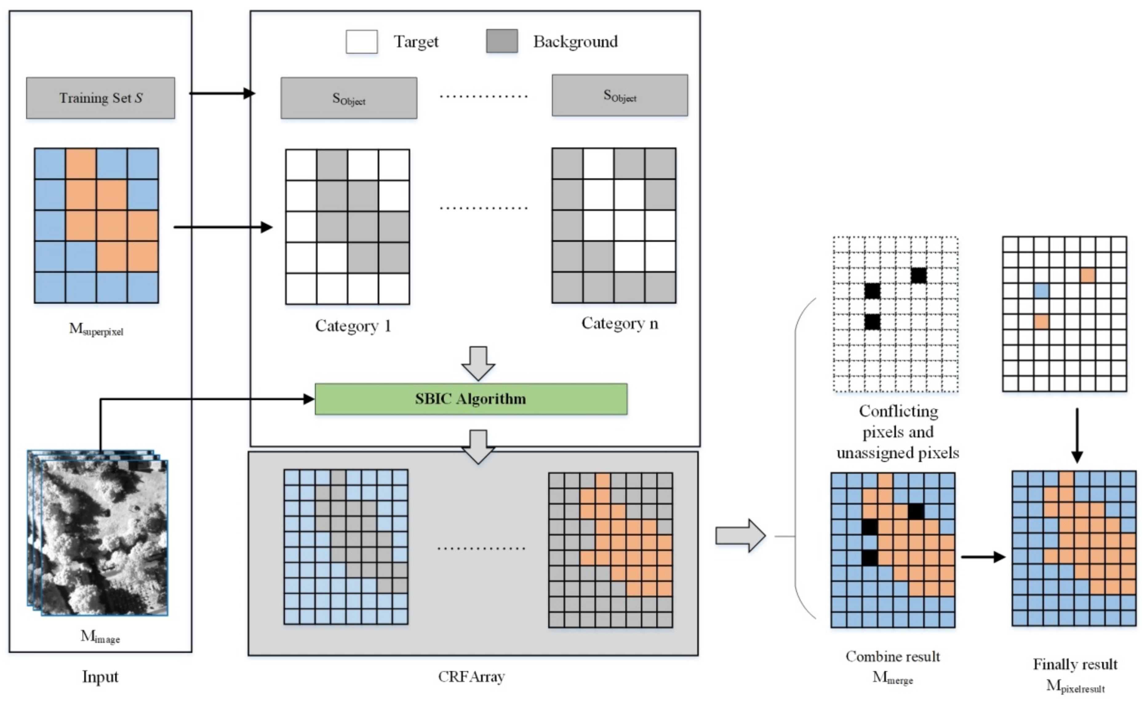
Algorithm 2 Restricted Conditional Random Field (RCRF)
Input: the remote sensing image Mimage; the superpixel classification result Msuperpixel; the sample set S; the maximum number of iterations Nmax; and the number of categories Ncategory.
Output: The segmented result Mpixelresult
CRFArray[Ncategory] = Initialize the array with Ncategory elements;
 for i in i: Ncategory {
  Define the ith category as the “target” and the other category as the “background”;
  Mlabel = transform Msuperpixel into a two-category superpixel image with “target” and “background” categories;
  Sobject = transform S into a two-category training set with “target” and “background” categories;
  Mresult = SBIC (Mimage, Mlabel, Sobject, Nmax);
  CRFArray[i] = fetch all the “target” category pixels in Mresult and change their category labels into the ith category;
 }
Mcrfresult = Use the fully connected CRF to segment Msuperpixel in Nmax iterations;
Mmerge = Combine all pixels and their category labels in CRFArray into a result image, and remove all conflicting pixels;
CPixels = Obtain conflicting pixels in CRFArray and assign each pixel’s category using the category of the Mcrfresult’s corresponding position pixel;
UPixels = Obtain unassigned pixels according to CRFArray (position in the result image and no corresponding category pixel in CRFArray) and assign each pixel’s category using the category of Msuperpixel’s corresponding position pixel;
Mpixelresult = Mmerge + (CPixels + UPixels);
 return Mpixelresult;
End
The RCRF algorithm exhibits two main characteristics when applied to remote sensing superpixel classification results. First, it can convert multi-category segmentation tasks into multiple two-category “target” and “background” segmentation tasks, thereby reducing the difficulty of determining the number of iterations for the CRF. Second, the SBIC algorithm is introduced to effectively control the segmentation output. The SBIC can effectively prevent excessive expansion or reduction of land covers in specific categories and overriding of small land covers.
Through these three main steps, when classifying a high-resolution remote sensing image, the CNN-RCRF not only takes full advantage of the CNN’s classification ability but also obtains a pixel-based remote sensing image classification result image.

3. Experiments

3.1. Algorithm Realization and Test Images

In this study, all the tested algorithms were implemented using Python 2.7. The deep learning algorithm was implemented based on the Keras extension package for Python, and the fully connected CRF algorithm was implemented based on the PyDenseCRF extension package for Python. An Intel-i5 2300/16 G/GeForce GT 730 computer was used to execute all the programs. To test the algorithms, this study adopts the “Semantic labelling contest of ISPRS WG III/4” dataset from the ISPRS and selects the two study images shown in Figure 4 from the dataset.
As shown in Figure 4a, an image from Vaihingen is adopted as study image 1. Its size is 1388 × 2555 and its spatial resolution is 9 cm. This image includes three bands: near-infrared (NIR), red (R) and green (G). As shown in Figure 4b, an image from Potsdam is adopted as research study image 2. Its size is 6000 × 6000 and its spatial resolution is 5 cm. This image includes: red (R), green (G), blue (B), infrared (I) and digital surface models (DSM) as test spatial features. Figure 4c,d present the corresponding ground truths for six categories: Impervious surfaces (IS), Building (B), Low vegetation (LV), Tree (T), Car (C), and Clutter/background (C/B). 400 samples are selected from each category based on the ground truth. Then, in these 400 samples, 200 samples are randomly selected as the training data and another 200 as the test data. Study image 1 contains five categories (study image 1 does not include the C/B category). The corresponding training dataset and test dataset each contain 200 × 5 = 1000 samples. Test image 2 contains six categories, and its corresponding training dataset and test dataset each contain 200 × 6 = 1200 samples.

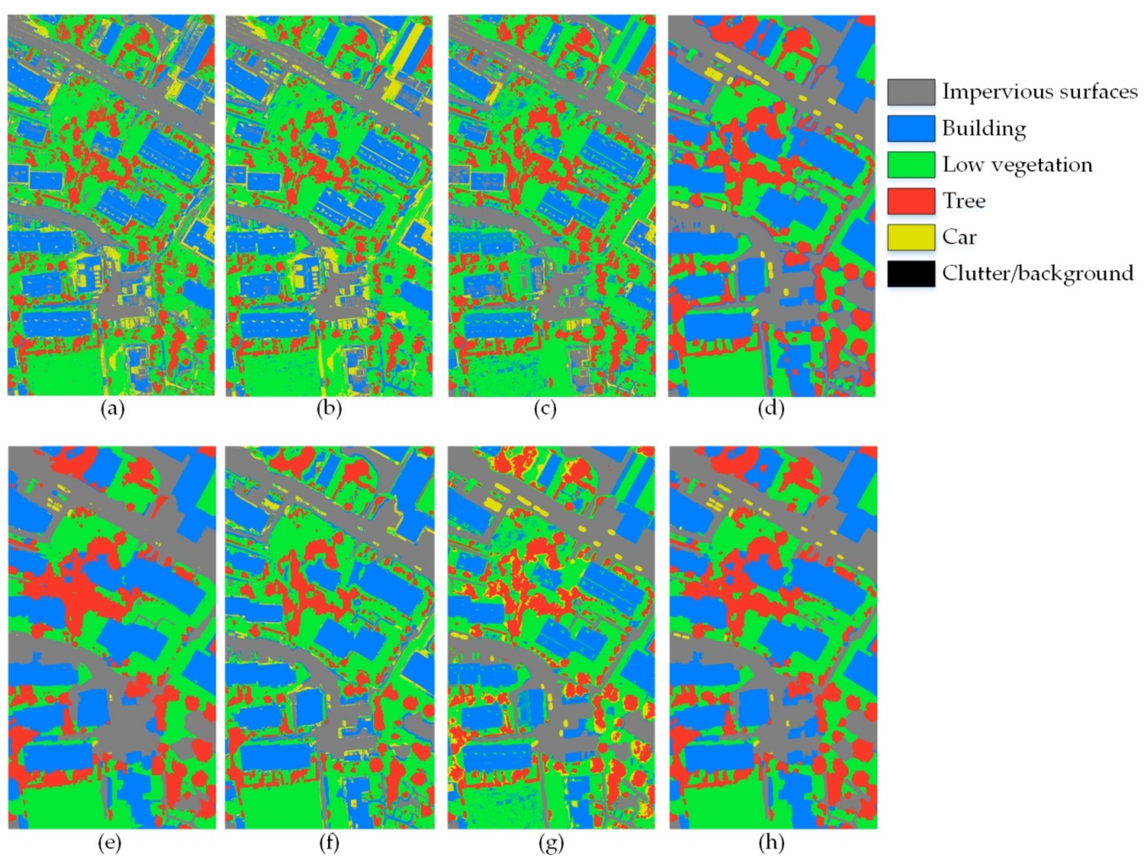
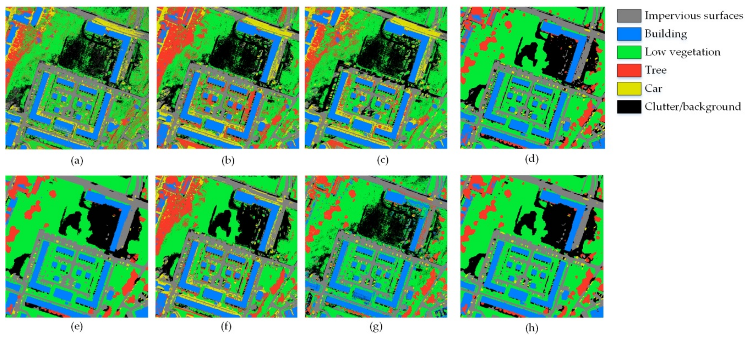
3.2. Comparison of Classification Results of Two Study Images

To evaluate the classification ability of the CNN-RCRF, this paper compares eight methods.
  • k-NN: In this algorithm, the number of neighbors is varied from 2 to 20, and the classification result with the best accuracy is selected as the final classification result.
  • MLP: MLP is composed of an input layer, a hidden layer, and an output layer. The input and hidden layers adopt ReLu as the transmission function, while the output layer adopts softmax as the transmission function.
  • SVM: The RBF function is adopted as the kernel function of the SVM.
  • Pixel-based CNN: For this algorithm, we adopt the same input feature map size and the same CNN model as are used for the CNN-RCRF. During image classification, each pixel in the image is taken as a central point and an image patch is obtained based on this central point. The CNN model obtains the image patch’s category label as the corresponding pixel’s category label.
  • CNN + CRF: This algorithm adopts the same input feature map size and the same CNN model as in CNN-RCRF to obtain the superpixel classification result image. The fully connected CRF segments the superpixel image into the pixel-based result.
  • CNN fusion MLP: This algorithm introduces the outputs of MLP and Pixel-based CNN, and then uses a fuzzy fusion decision method (proposed by reference [33]) to integrate the two algorithms’ results into a result image.
  • CNN features + MLP: This algorithm adopts the last layer of the CNN’s softmax output as the spatial features. Then, it uses MLP to obtain classification result based on the image original bands and these spatial features.
  • CNN-RCRF: The parameter Scaletarget is set to 5. The parameter Nmax is set to 10. To further test the relationship between the CNN input feature map size and classification result, the parameter Scale is set to: 9 × 9, 15 × 15, 21 × 21, 27 × 27, 33 × 33, 39 × 39, 45 × 45, and 51 × 51. Adopt best accuracy result among eight feature map size as CNN-RCRF‘s result.
k-NN, MLP and SVM are traditional shallow-model methods, and the pixel-based CNN, CNN + CRF, CNN fusion MLP, CNN feature + MLP, and CNN-RCRF are deep-model methods. The classification result images obtained by the eight methods for study image 1 are shown below.
As shown in Figure 5, there is a significant difference between the shallow-model methods and the deep-model methods in terms of the overall classification effect. Because the shallow-models take only the pixel band value into consideration, many misclassified pixels appear in the classification result images of the k-NN, MLP and SVM methods (which correspond to Figure 5a–c, respectively), the “salt-and-pepper effect” is obvious, and the land covers that have similar band values but different textures are poorly classified. For the deep models, the pixel-based CNN, CNN + CRF, CNN fusion MLP, CNN features + MLP and CNN-RCRF all adopt 33 × 33 as the input feature map size, and the continuity is significantly improved. As shown in Figure 5d, some details are missing from the land cover border, small land cover areas tend to be round, and some incorrect classifications are exaggerated, such as the trees surrounded by buildings in the lower-left part of result image. This result means that if the CNN is directly applied to the pixel-based classification, land cover deformation may occur. In Figure 5e, due to the excessive expansion of certain land covers during the CRF segmentation process, some small land covers are wrongly classified by the surrounding land covers. In Figure 5f, the classification errors in the MLP’s land cover boundary are still retained in the result, and the classification result shows no improvement compared to that of the pixel-based CNN. In Figure 5g, the fragmentation is more severe than in other deep-model methods, and there are still many errors at the boundary of the land cover. The classification result of CNN-RCRF is presented in Figure 5h. The classification results of the CNN-RCRF are the best among the eight algorithms, and it correctly classified almost all the land cover. In Figure 6, a feature map size of 33 × 33 is adopted as an example to compare the superpixel result image, the traditional fully connected CRF segmentation result image and the RCRF segmentation result image.
The fully connected CRF uses 10 iterations. The maximum number of iterations (Nmax) for RCRF is 10. Figure 6b shows the fully connected CRF result image and Figure 6c shows the RCRF result image. After segmentation by these two algorithms, the superpixel classification result image is refined. The algorithms both reduce the degree of roughness of the superpixel image; the boundaries of buildings and roads become smoother and the land cover shapes become clearer. In Figure 6d, four typical regions are chosen for a comparative analysis: the isolated superpixels misclassified as Building that appear at Region 1, Region 2 and Region 4 are rectified by both the fully connected CRF and RCRF. This result means that during the segmentation process, certain misclassified isolated superpixels can be rectified. However, the fully connected CRF segmentation has a series of problems: In Region 1, the excessive expansion of the low-vegetation area overrides some trees and some cars are covered by impervious surfaces, In Region 2, the small plots of low-vegetation area at the centre are covered by trees. In Region 3, the buildings whose colours are similar to the colours of the impervious surfaces are covered by impervious surfaces. In Region 4, the low-vegetation area covers two trees in the image. Compared with the CRF, the RCRF largely avoids such incorrect segmentations.
For study image 2, the classification results of the eight algorithms are compared in Figure 7.
In Figure 7a–c, the three shallow-model methods clearly distinguish buildings from other land covers based on the spatial features of test image 2; however, their classifications of other land cover types are poor: many low-vegetation, trees, clutter/background areas, cars and impervious surfaces are misclassified. These problems impair the overall classification results of the three shallow-model methods. CNN-RCRF adopts 39 × 39 as the input feature map size. As shown in Figure 7d–g, the result images of the five deep-model methods are significantly superior to those of the three shallow-model methods in terms of continuity. Nevertheless, boundary deformations and classification mistake due to exaggeration are still unavoidable in the pixel-based CNN, and some misclassified clutter/backgrounds surround other land covers. In the CNN + CRF result image, excessive expansion phenomena are observed, trees are misclassified as low-vegetation areas, and many cars are misclassified. The CNN fusion MLP and CNN features + MLP still cannot solve the problem of misclassification of land cover boundaries. Compared with the other methods, the CNN-RCRF achieves the best classification results.

4. Discussion

4.1. Comparison of Classification Accuracy

The classification accuracy of the eight methods for study image 1 and study image 2 is compared in Table 2:
As shown in Table 2, for study image 1, because only pixel band values are considered rather than pixel neighborhood information, the three shallow-model methods are unable to distinguish the land covers successfully, and they achieve lower classification accuracies. In particular, the accuracy of car classifications is very low. The k-NN’s classification accuracy is 67.6%, that of MLP is 68.3%, and SVM achieves 70.8%. The accuracy of the pixel-based CNN is 85.4%; boundary and outline distortions limit its accuracy to some extent. The accuracy of CNN + CRF reaches only 82.1%, which is lower than that of the pixel-based CNN. This result is due to the excessive expansion or reduction of some land covers during the CRF segmentation process. Compared to pixel-based CNN, the accuracy of CNN fusion MLP and CNN features + MLP did not change significantly (83.6% and 84.2%, respectively). Compared with the other methods, the CNN-RCRF achieves the highest accuracy, 90.1%. For test image 2, the spatial band values of buildings are significantly different from those of the other land covers; therefore, all the methods can identify them correctly. The building classification accuracy of the pixel-based CNN is slightly lower than that of the other algorithms because the boundaries of the land covers are slightly distorted. Consistent with test study image 1, the accuracies of the three shallow-model methods are lower than those of the deep models, and the CNN-RCRF achieves the highest accuracy of 90.3%.
Shallow-models cannot effectively classify high-resolution remote sensing images; it is very difficult to classify land cover with similar band values by single pixels. Thereby their classification accuracy is low. Deep models have better classification ability than shallow models, especially in the car category. These findings prompted us to utilize deep learning methods in the remote sensing classification field. Traditional pixel-based CNNs and CNN + RCRFs cannot handle land-cover boundaries well, leading to relatively low classification accuracy. CNN fusion MLP and CNN features + MLP rely on both the CNN’s and MLP’s classification ability. The land cover boundary problem still influences the classification result when the classification accuracy of the MLP at the land cover boundary is low. CNN-RCRF not only can take advantage of the CNN’s classification ability but can also avoid boundary or outline distortions, so CNN-RCRF outperforms the other algorithms in terms of classification accuracy.

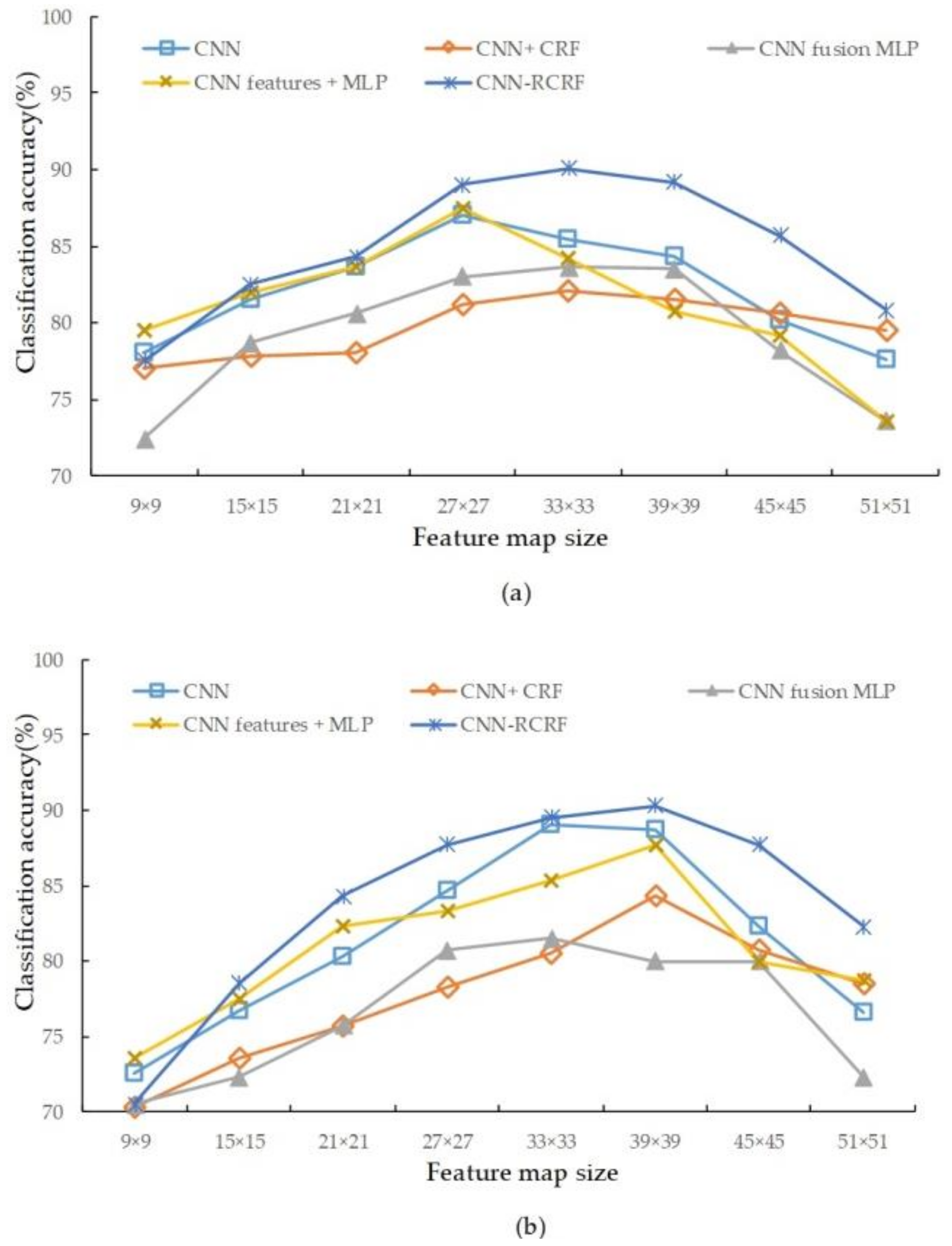
4.2. Comparison of Scale

For the five deep-model methods (CNN, CNN + CRF, CNN fusion MLP, CNN features + MLP and CNN-RCRF), the classification accuracy for the eight input scales is shown in Table 3:
The comparison of the classification accuracy of the three methods is shown in Figure 8.
According to Table 3 and Figure 8, the classification accuracies of the three deep-model methods are closely related to the scale of the input feature map; as the scale increases, the classification accuracy of the algorithms increases. After reaching a maximum point, the scale continues to increase (leading to an input feature map that contains more land covers), which leads to a decrease in classification accuracy. For the two study images, the accuracy of the CNN-RCRF is higher than those of the other two methods except for the smallest case (9 × 9), indicating that CNN-RCRF has a greater ability to improve classification accuracy. CNN + CRF has low classification accuracy in most cases, which means that CRF can hardly improve classification accuracy without solving the problem of traditional CRF; the curves of CNN fusion MLP and CNN features + MLP are similar to that of pixel-based CNN. Furthermore, in Figure 8a,b, the decrease in the CNN’s classification accuracy occurs at smaller scale than that for CNN-RCRF and CNN + CRF, which means that with increasing feature map scale, the land cover boundary deformation has an increasingly larger influence on classification accuracy. Moreover, as shown in Figure 8, the resolution of the image also influences the selection of the scale. The resolution of study image 1 is lower than that of study image 2; thus, the best scale for study image 1 is smaller than that of study image 2 for all three methods.
From the above analysis, it can be seen that the classification ability of a CNN is affected by the input feature map scale, too small and too large scale will negatively affect classification accuracy. Finding the best input scale of a remote image usually entails a trial and error strategy, which always requires a large number of classification experiments. The classification accuracy curve of CNN-RCRF gradually increases and then decreases. This characteristic can guide us in finding the best scale of CNN-RCRF. In future research, we plan to take the gradient of the CNN-RCRF classification accuracy curve into account and find the best scale of an image in relatively few experiments.

4.3. Comparison of Computation Time

In terms of computation time, each method was executed three times on the two study images, and the average execution time is adopted as the computation time for the method. The computation time of each method is separated into the training stage and classification stage. Because the pixel-based CNN and CNN + CRF adopt the CNN-CRF’s classification model, so CNN and CNN + CRF training time are same as that of CNN + CRF’s. The computation time of the CNN fusion MLP is composed of pixel-based CNN’s computation time, the MLP’s computation time and the image fusion time. The computation time of CNN features + MLP is composed of the pixel-based CNN’s computation time, spatial features construction time, and the new MLP model training and classification time. The computation time of the eight methods are shown in Table 4:
As shown in Table 4, the training and classification stages of the three shallow-model methods are notably shorter than those of the three deep models. k-NN does not require model training; therefore, its training stage consists only of reading and constructing the training dataset, and its computation time is the shortest among all the methods. The MLP and SVM methods are more complex than the k-NN, and their computation time are slightly longer. The pixel-based CNN’s image classification stage’s computation time is significantly longer than those of the other methods because it constructs an input feature map set and classifies it for every pixel in the image. For study image 1, the pixel-based CNN performs 1388 × 2555 = 3,546,340 classifications, and for study image 2, it performs 6000 × 6000 = 36,000,000 classifications, which is an enormous computational burden. On test image 2, the pixel-based CNN requires 163,138 s (more than two days); thus, the pixel-based CNN method cannot efficiently fulfil the task of classifying larger remote sensing images. Both CNN fusion MLP and CNN features + MLP are based on the pixel-base CNN’s result, so their computation time are slightly longer than that of a pixel-based CNN. The CNN + CRF and CNN-RCRF both adopt superpixel classification rather than pixel-based classification. On study image 1, they only need to perform ceil(1388/33) × ceil(2555/33) = 3354 classifications, and on study image 2 they need perform ceil(6000/39) × ceil(6000/39) = 23,716 classifications. Both are significantly lower than the pixel-based CNN. For the two study research images, the CNN + CRF takes 419 s and 1583 s, respectively, and the CNN-RCRF takes 506 s and 1744 s, respectively.
Based on the above comparisons, using a CNN to classify each pixel of a remote-sensing image will lead to a very large computational burden. With respect to computation time, the pixel-based CNN, CNN fusion MLP and CNN features + MLP have low application value because users would need to wait a very long time to classify an image. Conversely, CNN-RCRF can obtain a result in a relatively short time, and its computation times are more acceptable, indicating that the CNN-RCRF is more applicable to real-world remote sensing image classification tasks.

5. Conclusions

High-resolution remote sensing images usually contain large amounts of detailed information. Obtaining favorable classification results is difficult when relying only on the pixel band values; consequently, it is necessary to introduce neighborhood information into the classification process as context information. CNN’s convolutional layers and max-pooling layers give it the ability to consider a pixel’s neighborhood as context information, allowing it to discover deeper image characteristics. However, a CNN’s input is a feature map set, while its output is a category label; therefore, applying this structure directly to pixel-based remote sensing image classification will lead to boundary and outline distortions of the land covers in the result image. To classify high-resolution remote sensing images more effectively, this paper proposes the CNN-RCRF, which has two advantages. First, the CNN-RCRF uses a superpixel classification image, which can significantly reduce the number of classifications required to classify the entire image; hence, the classification speed of the CNN-RCRF is considerably faster than that of the pixel-based CNN method. Second, the CNN-RCRF adopts the RCRF algorithm to segment the superpixel classification result image. This approach avoids the boundary and outline distortions caused by pixel-based CNNs and the excessive expansion or shrinking of land covers caused by traditional fully connected CRFs. Thus, even small land cover areas (such as cars) can be correctly recognized by the CNN-RCRF. The experimental results show that the CNN-RCRF achieves higher classification accuracy compared to the k-NN, MLP, SVM, pixel-based CNN, CNN + CRF, CNN fusion MLP, and CNN features + MLP algorithms. Furthermore, the CNN-RCRF’s total time for classifying remote sensing images is also acceptable. These advantages give the CNN-RCRF algorithm a wider application range in high-resolution remote sensing classification fields.

Author Contributions

X.P. and J.Z. conceived and designed the experiments; J.Z. performed the experiments and analyzed the data; X.P. wrote the paper.

Acknowledgments

This research was jointly supported by the National Natural Science Foundation Youth Fund of China (61503044); Foundation of Jilin Provincial Science & Technology Department (20180101020JC; 20180622006JC); Foundation of Jilin Province Education Department (JJKH20170516KJ).

Conflicts of Interest

The authors declare no conflict of interest.

References

  1. Pan, X.; Zhang, S.Q.; Zhang, H.Q.; Na, X.D.; Li, X.F. A variable precision rough set approach to the remote sensing land use/cover classification. Comput. Geosci. 2010, 36, 1466–1473. [Google Scholar] [CrossRef]
  2. Tuia, D.; Pasolli, E.; Emery, W.J. Using active learning to adapt remote sensing image classifiers. Remote Sens. Environ. 2011, 115, 2232–2242. [Google Scholar] [CrossRef]
  3. Maggiori, E.; Tarabalka, Y.; Charpiat, G.; Alliez, P. Convolutional neural networks for large-scale remote-sensing image classification. IEEE Trans. Geosci. Remote Sens. 2017, 55, 645–657. [Google Scholar] [CrossRef]
  4. Blaschke, T. Object based image analysis for remote sensing. ISPRS J. Photogramm. 2010, 65, 2–16. [Google Scholar] [CrossRef]
  5. Liu, D.S.; Xia, F. Assessing object-based classification: Advantages and limitations. Remote Sens. Lett. 2010, 1, 187–194. [Google Scholar] [CrossRef]
  6. Johnson, B.; Xie, Z.X. Classifying a high resolution image of an urban area using super-object information. ISPRS J. Photogramm. 2013, 83, 40–49. [Google Scholar] [CrossRef]
  7. Hinton, G.E.; Osindero, S.; Teh, Y.W. A fast learning algorithm for deep belief nets. Neural Comput. 2006, 18, 1527–1554. [Google Scholar] [CrossRef] [PubMed]
  8. Long, J.; Shelhamer, E.; Darrell, T. Fully convolutional networks for semantic segmentation. In Proceedings of the Computer Vision and Pattern Recognition (CVPR), Boston, MA, USA, 7–12 June 2015; pp. 3431–3440. [Google Scholar]
  9. Sainath, T.N.; Kingsbury, B.; Saon, G.; Soltau, H.; Mohamed, A.R.; Dahl, G.; Ramabhadran, B. Deep convolutional neural networks for large-scale speech tasks. Neural Netw. 2015, 64, 39–48. [Google Scholar] [CrossRef] [PubMed]
  10. Silver, D.; Huang, A.; Maddison, C.J.; Guez, A.; Sifre, L.; van den Driessche, G.; Schrittwieser, J.; Antonoglou, I.; Panneershelvam, V.; Lanctot, M.; et al. Mastering the game of go with deep neural networks and tree search. Nature 2016, 529, 484–489. [Google Scholar] [CrossRef] [PubMed]
  11. Xiong, P.; Wang, H.R.; Liu, M.; Zhou, S.P.; Hou, Z.G.; Liu, X.L. ECG signal enhancement based on improved denoising auto-encoder. Eng. Appl. Artif. Intell. 2016, 52, 194–202. [Google Scholar] [CrossRef]
  12. Ijjina, E.P.; Mohan, C.K. Classification of human actions using pose-based features and stacked auto encoder. Pattern Recognit. Lett. 2016, 83, 268–277. [Google Scholar] [CrossRef]
  13. Wang, Y.Q.; Xie, Z.G.; Xu, K.; Dou, Y.; Lei, Y.W. An efficient and effective convolutional auto-encoder extreme learning machine network for 3D feature learning. Neurocomputing 2016, 174, 988–998. [Google Scholar] [CrossRef]
  14. Ma, X.R.; Wang, H.Y.; Geng, J. Spectral-spatial classification of hyperspectral image based on deep auto-encoder. IEEE J. Sel. Top. Appl. Earth Obs. Remote Sens. 2016, 9, 4073–4085. [Google Scholar] [CrossRef]
  15. Huang, W.; Xiao, L.; Wei, Z.H.; Liu, H.Y.; Tang, S.Z. A new pan-sharpening method with deep neural networks. IEEE Geosci. Remote Sens. Lett. 2015, 12, 1037–1041. [Google Scholar] [CrossRef]
  16. Chen, Y.S.; Lin, Z.H.; Zhao, X.; Wang, G.; Gu, Y.F. Deep learning-based classification of hyperspectral data. IEEE J. Sel. Top. Appl. Earth Obs. Remote Sens. 2014, 7, 2094–2107. [Google Scholar] [CrossRef]
  17. Romero, A.; Gatta, C.; Camps-Valls, G. Unsupervised deep feature extraction for remote sensing image classification. IEEE Trans. Geosci. Remote Sens. 2016, 54, 1349–1362. [Google Scholar] [CrossRef]
  18. Geng, J.; Fan, J.C.; Wang, H.Y.; Ma, X.R.; Li, B.M.; Chen, F.L. High-resolution SAR image classification via deep convolutional autoencoders. IEEE Geosci. Remote Sens. 2015, 12, 2351–2355. [Google Scholar] [CrossRef]
  19. Zhao, W.Z.; Du, S.H. Spectral-spatial feature extraction for hyperspectral image classification: A dimension reduction and deep learning approach. IEEE Trans. Geosci. Remote Sens. 2016, 54, 4544–4554. [Google Scholar] [CrossRef]
  20. Liu, Y.Z.; Cao, G.; Sun, Q.S.; Siegel, M. Hyperspectral classification via deep networks and superpixel segmentation. Int. J. Remote Sens. 2015, 36, 3459–3482. [Google Scholar] [CrossRef]
  21. Lv, Q.; Niu, X.; Dou, Y.; Xu, J.Q.; Lei, Y.W. Classification of hyperspectral remote sensing image using hierarchical local-receptive-field-based extreme learning machine. IEEE Geosci. Remote Sens. 2016, 13, 434–438. [Google Scholar] [CrossRef]
  22. Li, W.J.; Fu, H.H.; Yu, L.; Gong, P.; Feng, D.L.; Li, C.C.; Clinton, N. Stacked autoencoder-based deep learning for remote-sensing image classification: A case study of African land-cover mapping. Int. J. Remote Sens. 2016, 37, 5632–5646. [Google Scholar] [CrossRef]
  23. Shao, Z.F.; Deng, J.; Wang, L.; Fan, Y.W.; Sumari, N.S.; Cheng, Q.M. Fuzzy autoencode based cloud detection for remote sensing imagery. Remote Sens. 2017, 9, 311. [Google Scholar] [CrossRef]
  24. Chen, S.Z.; Wang, H.P.; Xu, F.; Jin, Y.Q. Target classification using the deep convolutional networks for SAR images. IEEE Trans. Geosci. Remote Sens. 2016, 54, 4806–4817. [Google Scholar] [CrossRef]
  25. Marmanis, D.; Datcu, M.; Esch, T.; Stilla, U. Deep learning earth observation classification using imageNet pretrained networks. IEEE Geosci. Remote Sens. 2016, 13, 105–109. [Google Scholar] [CrossRef]
  26. Wang, J.; Song, J.W.; Chen, M.Q.; Yang, Z. Road network extraction: A neural-dynamic framework based on deep learning and a finite state machine. Int. J. Remote Sens. 2015, 36, 3144–3169. [Google Scholar] [CrossRef]
  27. Han, X.B.; Zhong, Y.F.; Zhang, L.P. An efficient and robust integrated geospatial object detection framework for high spatial resolution remote sensing imagery. Remote Sens. 2017, 9, 666. [Google Scholar] [CrossRef]
  28. Cheng, G.; Zhou, P.C.; Han, J.W. Learning rotation-invariant convolutional neural networks for object detection in VHR optical remote sensing images. IEEE Trans. Geosci. Remote Sens. 2016, 54, 7405–7415. [Google Scholar] [CrossRef]
  29. Xia, G.S.; Hu, J.W.; Hu, F.; Shi, B.G.; Bai, X.; Zhong, Y.F.; Zhang, L.P.; Lu, X.Q. Aid: A benchmark data set for performance evaluation of aerial scene classification. IEEE Trans. Geosci. Remote Sens. 2017, 55, 3965–3981. [Google Scholar] [CrossRef]
  30. Qayyum, A.; Malik, A.S.; Saad, N.M.; Iqbal, M.; Abdullah, M.F.; Rasheed, W.; Abdullah, T.A.B.R.; Bin Jafaar, M.Y. Scene classification for aerial images based on CNN using sparse coding technique. Int. J. Remote Sens. 2017, 38, 2662–2685. [Google Scholar] [CrossRef]
  31. Zhao, W.Z.; Du, S.H. Scene classification using multi-scale deeply described visual words. Int. J. Remote Sens. 2016, 37, 4119–4131. [Google Scholar] [CrossRef]
  32. Pan, X.; Zhao, J. A central-point-enhanced convolutional neural network for high-resolution remote-sensing image classification. Int. J. Remote Sens. 2017, 38, 6554–6581. [Google Scholar] [CrossRef]
  33. Zhang, C.; Pan, X.; Li, H.; Gardiner, A.; Sargent, I.; Hare, J.; Atkinson, P.M. A hybrid MLP-CNN classifier for very fine resolution remotely sensed image classification. ISPRS J. Photogramm. Remote Sens. 2017, 140, 133–144. [Google Scholar] [CrossRef]
  34. Liu, Y.; Nguyen, D.; Deligiannis, N.; Ding, W.R.; Munteanu, A. Hourglass-shapenetwork based semantic segmentation for high resolution aerial imagery. Remote Sens. 2017, 9, 522. [Google Scholar] [CrossRef]
  35. Fu, G.; Liu, C.J.; Zhou, R.; Sun, T.; Zhang, Q.J. Classification for high resolution remote sensing imagery using a fully convolutional network. Remote Sens. 2017, 9, 498. [Google Scholar] [CrossRef]
  36. Shelhamer, E.; Long, J.; Darrell, T. Fully convolutional networks for semantic segmentation. IEEE Trans. Pattern Anal. Mach. Intell. 2017, 39, 640–651. [Google Scholar] [CrossRef] [PubMed]
  37. Liu, F.Y.; Lin, G.S.; Shen, C.H. CRF learning with CNN features for image segmentation. Pattern Recognit. 2015, 48, 2983–2992. [Google Scholar] [CrossRef] [Green Version]
  38. Bouvrie, J. Notes on Convolutional Neural Networks. 2014, pp. 1–9. Available online: http://people.csail.mit.edu/jvb/papers/cnn_tutorial.pdf (accessed on 10 December 2017).
  39. Alam, F.I.; Zhou, J.; Liew, A.W.C.; Jia, X.P. CRF learning with CNN features for hyperspectral image segmentation. In Proceedings of the 2016 IEEE International Geoscience and Remote Sensing Symposium (IGARSS), Beijing, China, 10–15 July 2016; pp. 6890–6893. [Google Scholar]
  40. Lafferty, J.D.; McCallum, A.; Pereira, F.C.N. Conditional random fields: Probabilistic models for segmenting and labeling sequence data. In Proceedings of the Eighteenth International Conference on Machine Learning (ICML 2001), Williams College, MA, USA, 28 June‒1 July 2001; pp. 282–289. [Google Scholar]
  41. Chen, L.C.; Papandreou, G.; Kokkinos, I.; Murphy, K.; Yuille, A. Semantic Image Segmentation with Deep Convolutional Nets and Fully Connected CRFs. In Proceedings of the International Conference on Learning Representations 2015 (ICLR 2015), San Diego, CA, USA, 7–9 May 2015; pp. 1–14. [Google Scholar]
  42. Krähenbühl, P.; Koltun, V. Efficient Inference in Fully Connected CRFs with Gaussian Edge Potentials. In Proceedings of the Advances in Neural Information Processing Systems 24 (NIPS 2011), Granada, Spain, 12–15 December 2011; pp. 1–9. [Google Scholar]
Figure 1. Process of obtaining pixel-based segmentation result via conditional random fields (CRF). (a) The results of CRF under ideal conditions; (b) The results of CRF under real conditions.
Remotesensing 10 00920 g001
Figure 2. Basic process of the convolutional neural network-restricted conditional random field algorithm (CNN-RCRF).
Remotesensing 10 00920 g002
Figure 3. Process of the RCRF algorithm.
Remotesensing 10 00920 g003
Figure 4. Two study images and their corresponding ground truth. (a) study image 1; (b) study image 2; (c) ground truth of study image 1; (d) ground truth of study image 2.
Remotesensing 10 00920 g004
Figure 5. Comparison of the classification result images of eight methods for study image 1. (a) k-NN; (b) MLP; (c) SVM; (d) Pixel-based CNN; (e) CNN + CRF; (f) CNN fusion MLP; (g) CNN features + MLP; (h) CNN-RCRF.
Remotesensing 10 00920 g005
Figure 6. Comparison of the superpixel result image, traditional fully connected CRF segmentation result image and RCRF segmentation result image. (a) superpixel result image; (b)traditional fully connected CRF result; (c) RCRF result; (d) Comparison of four typical positions.
Remotesensing 10 00920 g006
Figure 7. Comparison of the classification result images of eight methods for study image 2. (a) k-NN; (b) MLP; (c) SVM; (d) Pixel-based CNN; (e) CNN + CRF; (f) CNN fusion MLP; (g) CNN features + MLP; (h) CNN-RCRF.
Remotesensing 10 00920 g007
Figure 8. Comparison of the five deep-model methods in in eight feature map size. (a) Study image 1; (b) Study image 2.
Remotesensing 10 00920 g008
Table 1. Detailed information of the CNN model.
ComponentsLayersDetail Information
InputModel inputInput = A image patch which size is Scale × Scale and band number (channel number) is Nchannel
Ouput = Scale × Scale × Nchannel
1Group 1Convolutional layer 1Kernel = size is 3 × 3 with Nchannel channels
Kernel Number = 64 Transmission Function = Relu
Output = Scale × Scale × 64
Max-pooling layer 1Down-sampling size = 2 × 2
Output = Scale/2 × Scale/2 × 64
Group 2Convolutional layer 2Kernel = size is 3 × 3 with 64 channels
Kernel Number = 64 Transmission Function = Relu
Output = Scale/2 × Scale/2 × 64
Max-pooling layer 2Down-sampling size = 2 × 2
Output = Scale/4 × Scale/4 × 64
Ngroupnum groups of convolutional layers and max-pooling layers
2Flattening layerOutput = converts the previous layer’s feature maps into a one-dimensional neural structure
3MLPInput LayerNumber of Neurons = 128
Transmission function = Relu
Middle layerNumber of Neurons = 32
Transmission function = Relu
Output layerNumber of Neurons = Image’s category number
Transmission function = softmax
Table 2. Classification accuracy comparison of eight methods.
Study ImageMethodISBLVTCC/BOverall Accuracy (%)
Study Image 1k-NN78.580.580.570.028.5/67.6
MLP80.575.581.570.533.5/68.3
SVM82.582.082.579.527.5/70.8
Pixel-based CNN83.587.590.583.582.0/85.4
CNN + CRF85.590.593.582.558.5/82.1
CNN fusion MLP84.588.590.084.570.5/83.6
CNN features + MLP83.586.589.579.582.0/84.2
CNN-RCRF87.591.592.589.589.5/90.1
Study Image 2k-NN70.593.072.074.024.080.569.0
MLP72.093.070.079.527.082.570.7
SVM73.593.073.575.539.584.573.3
Pixel-based CNN90.591.589.585.587.587.588.7
CNN + CRF89.593.090.583.560.588.584.3
CNN fusion MLP89.593.081.587.040.588.580.0
CNN features + MLP90.593.084.582.588.087.587.7
CNN-RCRF90.593.090.587.589.590.590.3
Table 3. Classification accuracy comparison of deep-model methods for eight feature map sizes.
Study ImageFeature Map SizeClassification Accuracy (%)
Pixel-Based CNNCNN + CRFCNN Fusion MLPCNN Features + MLPCNN-RCRF
Study Image 19 × 9787772.479.577.5
15 × 1581.577.878.78282.5
21 × 2183.67880.683.684.3
27 × 278781.28387.589
33 × 3385.482.183.684.290.1
39 × 3984.381.583.580.789.2
45 × 4580.280.678.279.285.7
51 × 5177.679.573.673.680.8
Study Image 29 × 972.570.370.573.570.5
15 × 1576.773.572.377.578.5
21 × 2180.375.775.782.384.3
27 × 2784.778.380.783.387.7
33 × 3389.080.581.585.389.5
39 × 3988.784.380.087.790.3
45 × 4582.380.780.080.087.7
51 × 5176.678.572.378.782.3
Table 4. Comparison of the computation times of the eight methods.
Study ImageMethodComputation Time (Seconds)
TrainingClassificationTotal
Study Image 1k-NN73648
MLP183149
SVM27182209
Pixel-Based CNN17515,35215,527
CNN + CRF175244419
CNN fusion MLP19315,44315,635
CNN features + MLP17515,42415,599
CNN-RCRF175331506
Study Image 2k-NN13321334
MLP29374403
SVM41702743
Pixel-Based CNN243162,895163,138
CNN + CRF24313401583
CNN fusion MLP272163,815164,087
CNN features + MLP243163,565163,808
CNN-RCRF24315011744

