Aircraft Type Recognition in Remote Sensing Images Based on Feature Learning with Conditional Generative Adversarial Networks

Abstract

Aircraft type recognition plays an important role in remote sensing image interpretation. Traditional methods suffer from bad generalization performance, while deep learning methods require large amounts of data with type labels, which are quite expensive and time-consuming to obtain. To overcome the aforementioned problems, in this paper, we propose an aircraft type recognition framework based on conditional generative adversarial networks (GANs). First, we design a new method to precisely detect aircrafts’ keypoints, which are used to generate aircraft masks and locate the positions of the aircrafts. Second, a conditional GAN with a region of interest (ROI)-weighted loss function is trained on unlabeled aircraft images and their corresponding masks. Third, an ROI feature extraction method is carefully designed to extract multi-scale features from the GAN in the regions of aircrafts. After that, a linear support vector machine (SVM) classifier is adopted to classify each sample using their features. Benefiting from the GAN, we can learn features which are strong enough to represent aircrafts based on a large unlabeled dataset. Additionally, the ROI-weighted loss function and the ROI feature extraction method make the features more related to the aircrafts rather than the background, which improves the quality of features and increases the recognition accuracy significantly. Thorough experiments were conducted on a challenging dataset, and the results prove the effectiveness of the proposed aircraft type recognition framework.

1. Introduction

With the rapid development of remote sensing technology, the quality and quantity of remote sensing images have improved significantly, which greatly promotes the progress of remote sensing image interpretation. Aircraft type recognition is one of the important issues in this field, and it has been widely used in both civil and military applications. However, due to the complex backgrounds, shadows, illumination changes, and other factors in remote sensing images, this task still has many challenges.

In recent years, many effective methods have been proposed to tackle the aircraft type recognition task. Some methods are designed based on handcrafted features. For example, Hsieh et al. [1] proposed a hierarchical classification algorithm based on four different features: wavelet transform, Zernike moment, distance transform, and bitmap. In Reference [2], a coarse-to-fine method is built to integrate the high-level information for aircraft type recognition. A method using artificial bee colony algorithm with an edge potential function is proposed in Reference [3] to deal with this problem. Although these methods achieve good results, they rely heavily on handcrafted features, and thus lack generalization and representation ability, which confines the effectiveness of these algorithms.

Deep learning methods have also been introduced to aircraft type recognition in recent studies. Wang et al. [4] proposed a self-organizing neural network cooperating with a support vector machine (SVM) to recognize aircrafts. Fang et al. [5] adopted a back propagation neural network and a series of preprocessing methods to deal with this problem. Additionally, multi-layer perception [6] and the deep belief net (DBN) [7] have been applied to recognition tasks. However, the networks used in the aforementioned methods are not deep enough to learn robust features for recognizing various aircrafts in complex backgrounds. Meanwhile, many deep convolutional neural networks (CNNs) [8,9,10,11] have achieved outstanding performance on image classification tasks, but these models must be trained on large-scale datasets [12,13] with category labels. It is quite expensive and time-consuming to acquire such large-scale datasets, since it requires a great deal of expertise to label aircrafts of different types.

There are also many template matching methods designed to tackle the recognition problem, since each type of aircraft has a fixed and unique shape in remote sensing images. Wu et al. [14] proposed a jigsaw reconstruction method to extract aircrafts’ shapes, and then match them with standard templates. Zhao et al. [15] designed a keypoint detection model based on CNNs, and a keypoint matching method to recognize aircrafts. Furthermore, Zuo et al. [16] built a template matching method using both aircrafts’ keypoints and segmentation results, which provided more detailed information to improve recognition accuracy. Although these methods have achieved good performance on certain datasets, they cannot effectively tackle images without resolution, which severely limits their practicality.

Currently, many aircraft images have been accumulated in remote sensing, but only a small portion of them are labeled with type information. Although template matching methods can work without type labels, they lack practicality in actual applications. The end-to-end deep models achieve good performance in natural image classification, however, they always require a large amount of data labeled with types. Given the current situation of remote sensing data, they cannot perform at their full potential. Therefore, it is necessary to build a model to learn robust representative features from unlabeled data for aircraft recognition. A generative adversarial network (GAN) is a potential option.

GANs, first proposed in Reference [17], train both a generator and a discriminator together, adversarially. To make GANs more suitable for image processing, Radford et al. [18] designed a deep convolutional generative adversarial network (DCGAN), and they applied it to image classification tasks. Driven by the effectiveness of GANs, several methods [19,20] based on conditional GANs have been proposed to tackle image-to-image tasks. These methods usually take pixel-wise semantic labels of images as the GANs’ conditional input. Benefiting from semantic labels, the conditional GANs can obtain more information about targets than ones which only take random noise as input. Thus, conditional GANs can generate images with higher quality and learn more robust and distinctive features to represent targets, which are potentially useful in classification tasks. However, there are still some obstacles to applying conditional GANs to aircraft type recognition tasks. First, pixel-wise semantic labels are too expensive to be acquired. Additionally, the learned features need to be further refined to distinguish similar aircrafts.

In this paper, we propose an aircraft type recognition framework based on a conditional GAN and SVM [21]. The proposed framework can learn representative features from images without type labels, allowing it to generate features more related to aircrafts. This significantly improves the recognition accuracy. Experiments show that our method outperforms state-of-the-art methods on a challenging dataset without using image resolution. The main contributions of this paper are as follows:

• We propose a framework to deal with the aircraft type recognition problem, which can learn distinctive features for aircraft recognition from abundant data without type labels. Only a modest number of labeled samples are required to build the recognition model with strong generalization ability.
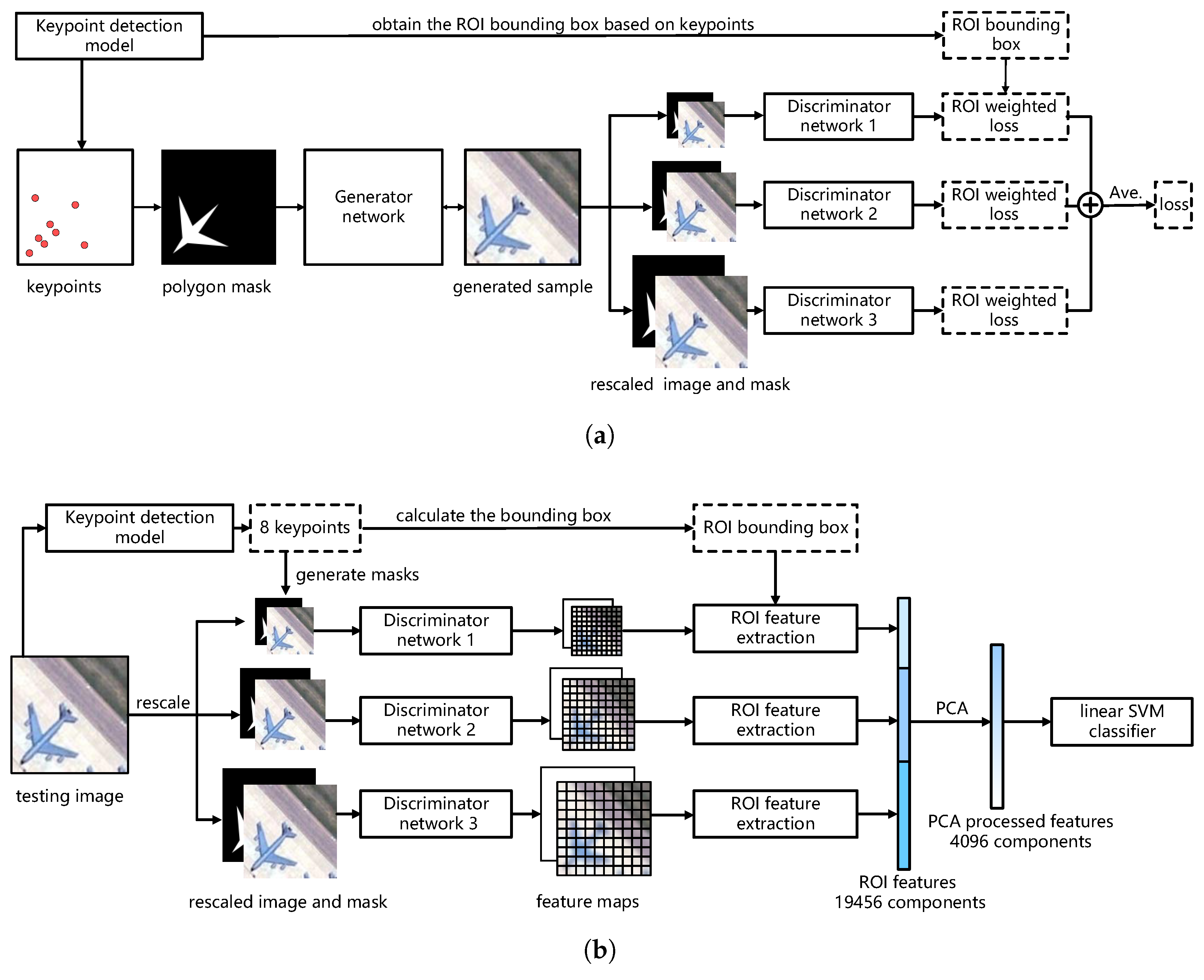
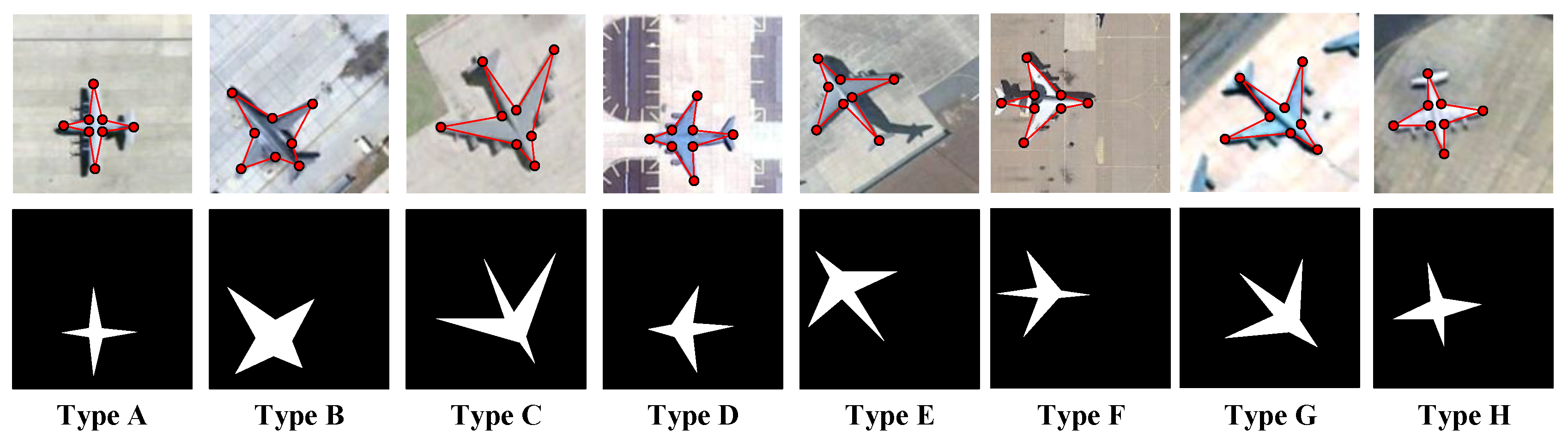
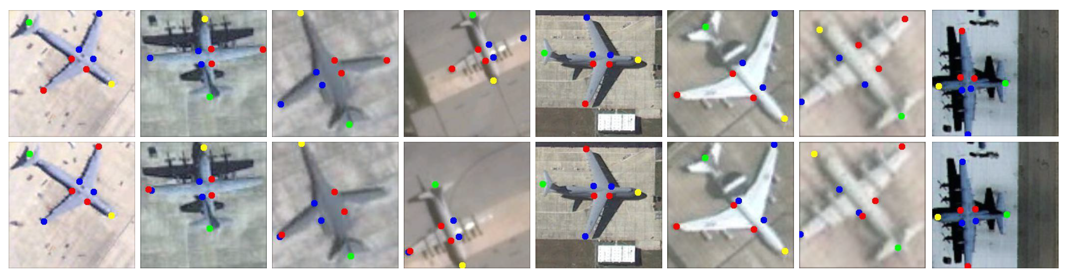
• We build a model to detect aircraft keypoints in $256\times 256$ images by generating heat maps. This improves the keypoints’ precision significantly by integrating both local and global features. Meanwhile, we design a strategy to correct the incorrect detections between symmetric keypoints (e.g., left and right wingtips), which further refines the model’s performance.
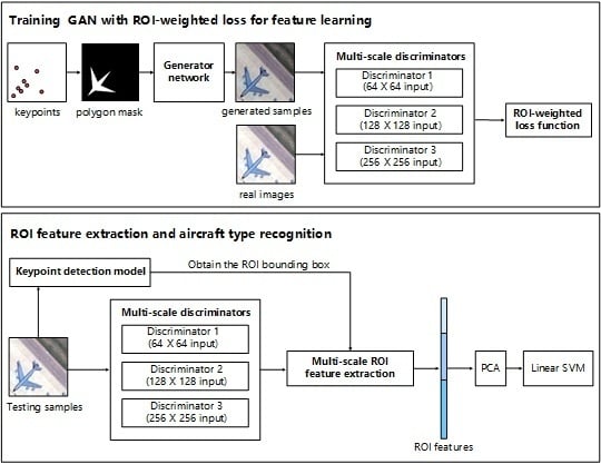
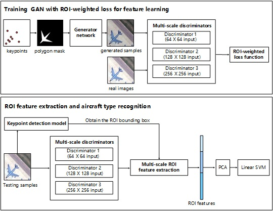
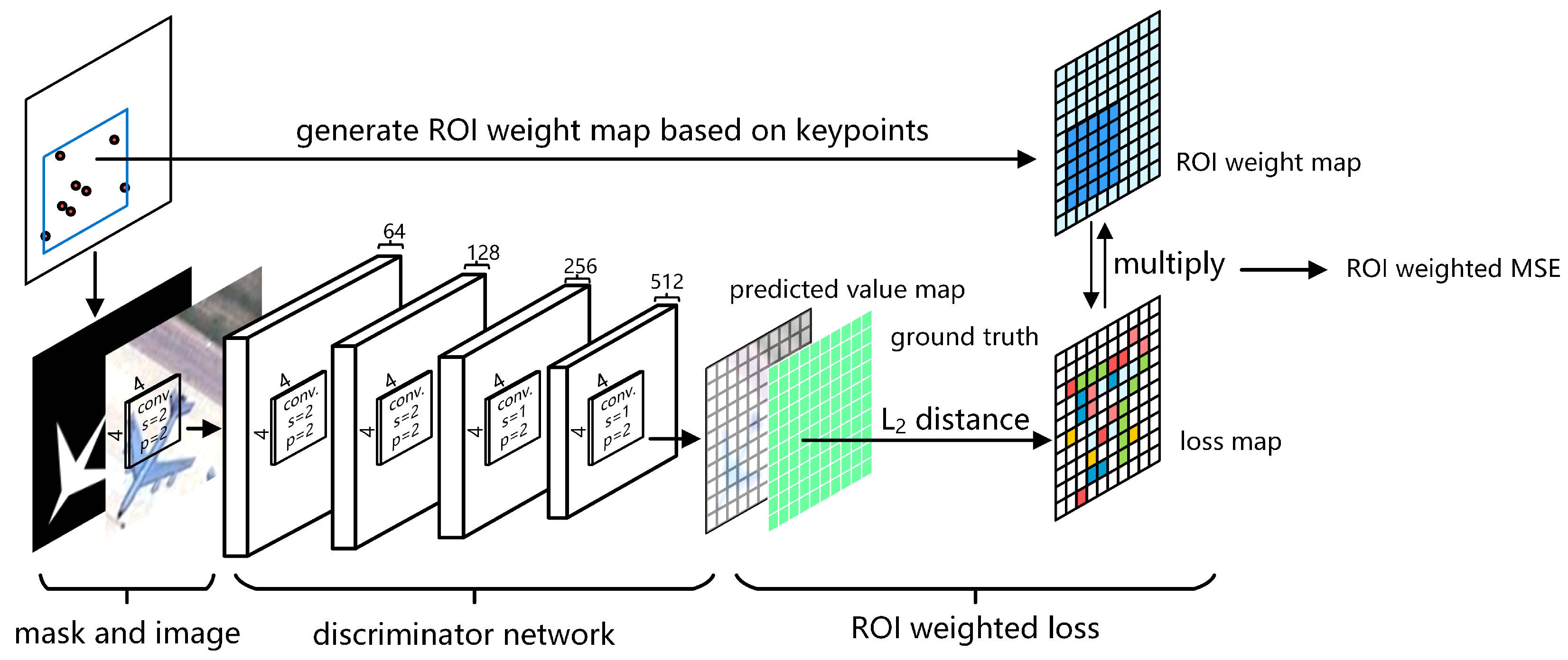
• We build a conditional GAN model based on Reference [20] to learn aircraft features. First, we replace the pixel-wise semantic labels with the masks generated by keypoints as the conditional input, which avoids the heavy labeling work. Then, to learn more representative features, an region of interest (ROI)-weighted loss function is designed to make the model focus on the regions of aircrafts instead of the background.
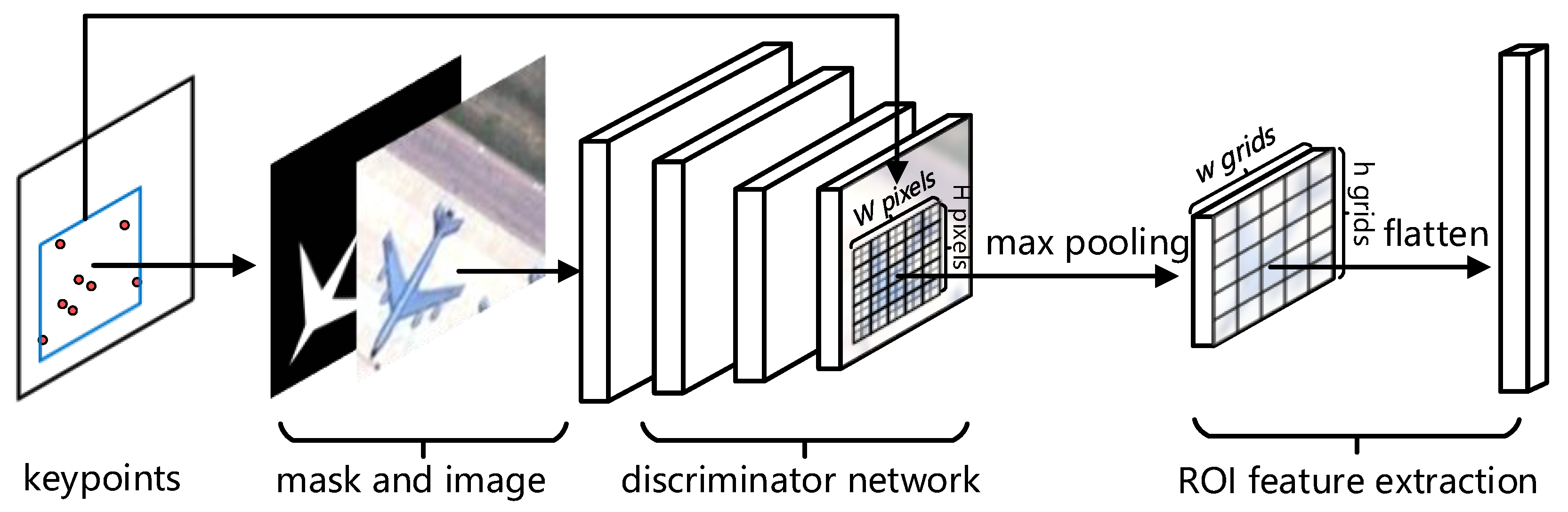
• To promote the quality of features, we design a method named ROI feature extraction to extract multi-scale features in the exact regions of the targets, which can eliminate the effects of complex backgrounds and deal with aircrafts of different scales and resolutions.

The rest of this paper is organized as follows: the framework and important parts of our method are detailed in Section 2. Section 3 outlines the experimental test of our approach and related analyses. Section 4 discusses some noteworthy issues of our work, based on the experimental results. Finally, the paper concludes in Section 5.

2. Proposed Method

The framework of our method is presented in Figure 1. First, we build a keypoint detection model based on an hourglass network [22] to detect an aircraft’s eight keypoints, consisting of the nose, tail, left wingtip (LW), right wingtip (RW), and the four joints of the wings and fuselage, as shown in Figure 2. The keypoint detection results play an important role in both GAN feature learning and the feature extraction stage.

Then, as shown in Figure 1a, a conditional GAN based on Reference [20] is trained to learn relevant aircraft features. The GAN’s generator takes aircraft masks generated by the keypoints as input and produces generated samples, while the GAN’s discriminators learn features by distinguishing generated samples from real images. To deal with aircrafts of different scales and resolutions, three different discriminators are established to learn multi-scale features. The generator and discriminators are trained jointly by minimizing the ROI-weighted loss function, which is designed based on the ROI bounding boxes generated by the keypoints, and enhances the correlation between the features and the aircrafts.

Finally, as shown in Figure 1b, we extract features from the GAN’s discriminators and build an SVM classifier to identify aircraft types. Specifically, the input images are rescaled and conveyed to the three trained discriminators to get the feature maps. Then, based on the ROI bounding boxes, the ROI feature extraction method processes the feature maps and produces representative features. Then, we adopt principal component analysis (PCA) to reduce the features’ dimensions and train an SVM classifier with the reduced features for aircraft recognition. The important parts of the framework are detailed in the following sub-sections.

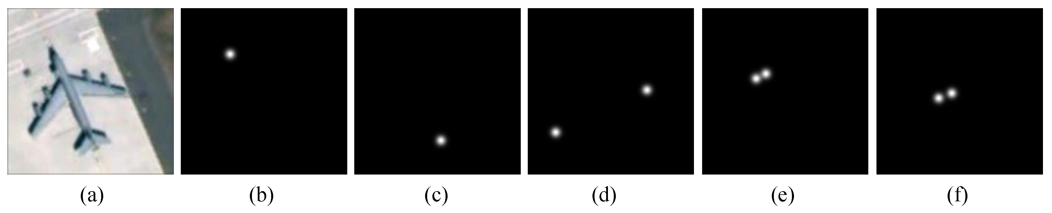
2.1. Aircraft Keypoint Detection

Aircraft keypoint detection methods are proposed in Reference [15,16]. Specifically, they first resize images to $40\times 40$, and then regress the keypoint coordinates directly using CNN models. Then, the keypoints are transformed back to the original images and used to recognize aircraft types. However, the methods in References [15,16] use pooling layers to process the whole feature maps from the previous layers. This operation ignores the local features learned by low layers, which are important to keypoint detection tasks. Although the method in Reference [16] adopts shortcut connections, it can only deliver local features to nearby higher layers. Thus, many of the local features from the low layers are still lost in the final layer, which affects the precision of the keypoints. Additionally, the resizing and transformation steps lead to inevitable errors.

As mentioned above, we make extensive use of aircraft keypoints in our GAN feature learning and feature extraction, so accuracy in locating the keypoints is crucial to our work. To avoid resizing and transformation errors, we detect aircraft keypoints directly in $256\times 256$ images instead of the $40\times 40$ images used in the previous methods. Since regression networks neglect the local features of low layers, we adopt the hourglass model of Reference [22] as the basic keypoint detection network. It uses a number of convolutional layers and residual blocks to build an encoder-decoder network. Then, it makes use of skip layers to combine the features of the low and high layers. Because the network preserves the spatial information on different scales, it provides more detailed features to locate keypoints precisely. For more details about the structure of the hourglass model, we refer the reader to Reference [22].

Instead of regression, the hourglass network first generates one heat map for each keypoint, and then finds the location of the maximum value in each heat map as the keypoint’s coordinates. For aircrafts in remote sensing images (which are highly symmetric), the model sometimes makes incorrect detections between symmetric points. Taking wingtips as an example, when we detect the left wingtip, the heat map may predict the maximum value at the position of the right wingtip, because they are very similar. To deal with this problem, we detect the pair of symmetric keypoints in a single heat map. An example of the ground truths of the keypoint heat maps are shown in Figure 3. The nose and tail are predicted in different heat maps separately, while the wingtips and symmetric joints are predicted together in the same heat maps. The values of a ground truth map are generated by:

$$S_{i,j}=exp\left(-\frac{{∥p-x_{i,j}∥}_2^2}{{\sigma }^2}\right),$$

(1)

where $∥.∥$ represents 2-norm, p presents the position of the keypoints, $x_{i,j}$ is the coordinate of a pixel in the heat map, $S_{i,j}$ is the value of that pixel, and we use $\sigma$ to control the activating area of a keypoint in the heat map (the white area in Figure 3). For the symmetric keypoints, the values are the sum of the $S_{i,j}$ calculated for the two keypoints separately. To avoid the overlap between symmetric keypoints’ activating areas, we calculate the minimum distance between two symmetric joints of all samples in the training dataset, and we set $\sigma$ to about half of this minimum distance, which in our case leads to $\sigma =5$ pixels.

Next, we get the keypoint positions from the heat maps following Algorithm 1. For a single keypoint, the maximum activating location of the heat map is predicted as the keypoint’s position. For symmetric keypoints, we first find the max activating location as the first keypoint. Then, we set the values of the heat map near this first keypoint to 0, where the neighborhood of the keypoint is taken to be a circle centered on the found keypoint with a radius of $r=5$ pixels, in accordance with the $\sigma$ value. After that, we find the other maximum activating location, which is taken as the location of the second keypoint.

Since we predict symmetric keypoints together, we must distinguish which is the right or left keypoint relative to the fuselage. We make use of the vector cross-product to distinguish them. Specifically, we calculate the vector cross-product between the vector from tail to nose and the vector from a keypoint to its symmetric keypoint. If the result is positive, the second vector is from the right to the left, and if the result is negative, the direction of the second vector is reversed.

Experiments show that the accuracy of keypoints improves greatly compared with previous methods, which builds a solid foundation for the GAN feature learning and feature extraction methods.

Algorithm 1 The procedure of obtaining keypoints from heat maps.

Input: Five heat maps Output: The eight aircraft keypoint coordinates  1: Nose heat map: Find the position of the maximum value as the nose’s coordinate $(p_x^n,p_y^n)$.  2: Tail heat map: Find the position of the maximum value as the tail’s coordinate $(p_x^t,p_y^t)$.  3: Calculate the standard direction vector $\overrightarrow{d_0}$= $(p_x^n-p_x^t,p_y^n-p_y^t)$  4: for each heat map of symmetric keypoints do  5:  Find the position of the maximum value as the left coordinate $(p_x^l,p_y^l)$.  6:  Set the value to 0 in a circle whose center is $(p_x^l,p_y^l)$ and radius is 5 pixels.  7:  Find the position of the maximum value as the right coordinate $(p_x^r,p_y^r)$.  8:  Calculate the direction vector $\overrightarrow{d_i}$= $(p_x^l-p_x^r,p_y^l-p_y^r)$.  9:  if $\overrightarrow{d_0}\times \overrightarrow{d_i}$ < 0 then 10:   Swap the left and right coordinates. 11:  end if 12: end for

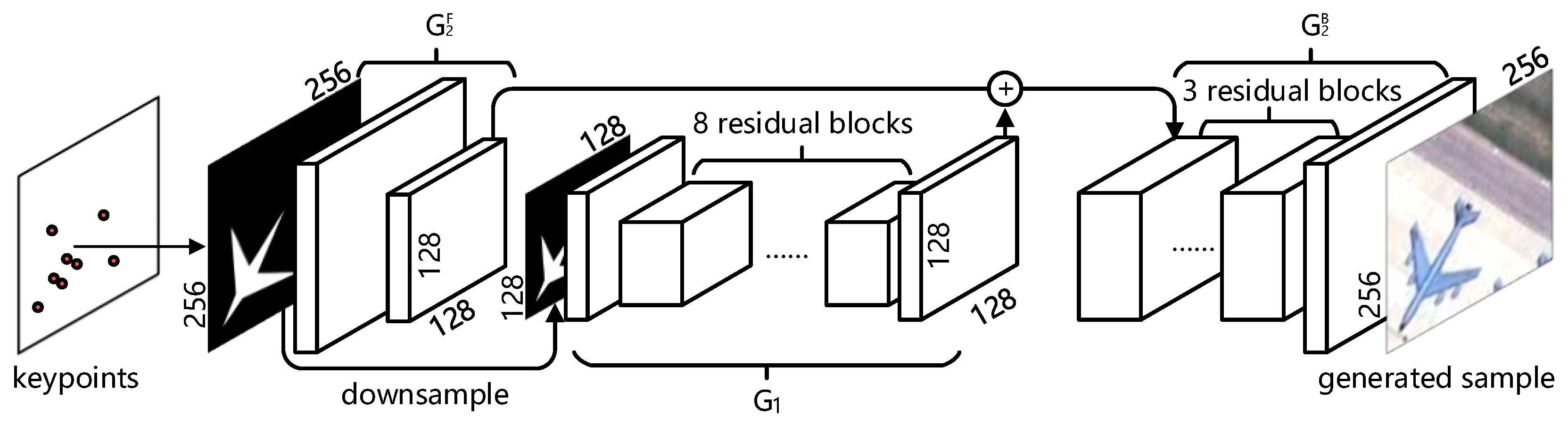
2.2. Conditional GAN with ROI-Weighted Loss Function

GANs were previously proposed in Reference [17]. In contrast to other deep learning methods, GANs train two networks, called the discriminator D and the generator G, at the same time and adversarially. The generator is used to capture the data distribution, and the discriminator aims to estimate the probability that a sample comes from the data rather than G.

To learn a generator distribution $p_g$ over data x, the generator builds a mapping function $G(z,{\theta }_g)$ from a prior noise distribution $p_z\left(z\right)$ to the data space. The discriminator $D(\widehat{x},{\theta }_d)$ takes either raw data x or the generated samples $G(z,{\theta }_g)$ as the input $\widehat{x}$, and outputs the probability that $\widehat{x}$ comes from training data rather than from $p_g$. During training, the parameters of D and G are updated separately. Specifically, we adjust the parameters of D to assign correct labels to both the training data and samples from G and we adjust the parameters of G to minimize $log(1-D(G\left(z\right)\left)\right)$. The training procedure is formulated as:

$$\underset{G}{min}\underset{D}{max}V\left(G,D\right)=E_{x\sim p_{\mathrm{data}}\left(x\right)}\left[logD\left(x\right)\right]+E_{z\sim p_z\left(z\right)}\left[log\left(1-D\left(G\left(z\right)\right)\right)\right].$$

(2)

where $V(G,D)$ is the loss function of the GAN, and $E(.)$ is the expectation.

Based on this basic idea, many improved GANs have been proposed to deal with different problems, such as the conditional GAN [23], improved GAN [24], DCGAN [18], and WGAN [25]. In image-to-image tasks [19,20], an image-conditional GAN is the most popular choice. This method aims to translate an input image from one domain into another domain given input–output image pairs as the training dataset.

In this paper, in contrast to previous methods, we pay more attention to learning robust features of aircrafts using discriminators rather than generating samples. Thus, we build an image-conditional GAN based on that of Reference [20]. The proposed GAN consists of a generator and three discriminators. The generator takes aircrafts’ masks as input, and generates high-quality aircraft samples. The discriminators take both images and masks as input, and learn representative features by distinguishing samples generated by the generator from the real images. Note that the discriminators do not need to identify each aircraft’s type, so type labels are not used in the GAN training procedure.

In image-to-image tasks, pixel-wise semantic labels are often taken as input. The pixel-wise semantic labels are acquired by precisely assigning a class label for every pixel in the training images. This kind of label can represent the refined shapes and outlines of objects, but they are quite expensive and time-consuming to obtain. In this paper, we replace the pixel-wise semantic labels with coarse labels generated by the aircrafts’ keypoints. Figure 2 shows some examples of the coarse labels. To obtain them automatically, a polygon is generated based on the keypoints, on an empty image with the same size as the corresponding aircraft image. The values inside the polygon are set to 1, while the values outside are set to 0. Since the coarse labels we use are quite different from the widely used pixel-wise semantic labels, we name the coarse labels as masks to avoid ambiguity. Although the binary masks are coarse, they still provide a great deal of important information about the aircrafts, such as basic shapes, berthing locations, and directions, which are all helpful for the generator to control generative sample patterns and improve their quality.

The architecture of the generator is shown in Figure 4. The generator consists of two components, marked as $G_1$ and $G_2$. $G_1$ is responsible for learning global features, while $G_2$ focuses more on local features. $G_1$ takes a downsampled mask of size $128\times 128$ as input, and produces $128\times 128$ feature maps. $G_2$ is decomposed into two sub-networks: $G_2^F$ and $G_2^B$. $G_2^F$ takes the original masks of size $256\times 256$ as input and produces feature maps of size $128\times 128$. Then, we add the $128\times 128$ feature maps from $G_1$ and $G_2^F$ together, and convey the sum to $G_2^B$ to produce the final generated samples. Such a multi-resolution pipeline has been widely used in GAN architectures [20,26,27,28,29]. In our work, we also use this strategy to improve the performance of the generator. Benefiting from the cooperation of $G_1$ and $G_2$, which concentrate on features of different resolution, the generator can produce samples with higher quality.

To deal with aircrafts of different scales and resolutions, the proposed GAN contains multiple discriminators, which have an identical network architecture as shown in Figure 5. Each discriminator contains five convolutional layers with a kernel size of $4\times 4$ and a padding size of 2. The first three layers have strides of 2 and others have strides of 1. All of the layers are equipped with batch normalization and a rectified linear unit (ReLU) except for the last layer. The discriminators take images of different sizes and their corresponding masks as input. To increase the distinctiveness of features, we set the input images’ sizes as different integer powers of 2. To avoid heavily mixing the aircraft and background information in the feature maps of the discriminators, we only downsample the input twice. Therefore, we build three different discriminators and set the input image sizes to $256\times 256$, $128\times 128$, and $64\times 64$. The discriminator with the larger input will focus more on the local features, while the discriminator with smaller input is inclined to learn global features. Benefiting from the cooperation of the three discriminators, the learned features are strong enough to represent aircrafts of different scales and resolutions.

As shown in Figure 2, some aircrafts only occupy small regions in the images. They can be easily ignored by the discriminator networks. Therefore, we input the images along with the masks to make the networks concentrate on the aircrafts rather than the background. To further deal with this problem, an ROI-weighted loss function is carefully designed based on the loss function proposed in LSGAN [30]. Specifically, as shown in Figure 5, for an input image, we first create a matrix with the same size as the outputs of the discriminators which is initialized to the value 1 at all locations. Then, we set the values of the ROI in the matrix to $\lambda$, where the ROI is obtained by finding the minimum outer rectangle of the detected keypoints and adjusting according to the appropriate scaling ratio. The result of this process is the ROI weight map in Figure 5, where the ROI is annotated with the deep blue color. Finally, we multiply the matrix with the calculated loss map element-by-element, and calculate the average. The loss function is formulated as:

$$L=\frac{1}{MN}\sum _{i=1}^M\sum _{j=1}^N{w}_{ij}{\left(p_{ij}-{\widehat{p}}_{ij}\right)}^2,$$

(3)

where M and N are the width and height of the matrix, $p_{ij}$ represents the value of the predicted value map, ${\widehat{p}}_{ij}$ represents the values of the ground truth, and $w_{ij}$ represents the values of the ROI weight map matrix, all at the point $i,j$. Finally, $w_{ij}$ takes a value of either 1 or $\lambda$.

In particular, we adopt rectangular regions rather than polygon masks in the weight computation. Since the values of feature maps are calculated by convolution, many feature values around the position of an aircraft are also related with the aircraft. Besides, rectangular regions match with the ROI feature extraction method, which is detailed in Section 2.3.

We train the model end-to-end by minimizing the ROI weighted loss function following the procedure of Reference [20]. Experiments demonstrate that our model is able to extract representative features to distinguish different aircrafts.

2.3. Multi-Scale ROI Feature Extraction

Considering that the trained discriminators can distinguish real images from generated samples, the features learned by the discriminators can represent various aircrafts. However, the dimension of features is too large to be manipulated. Additionally, the features not only contain information about the aircrafts, but also contain redundant information related to the background. Therefore, it is necessary to refine the features before they are applied to aircraft type recognition.

In this section, we propose a method named ROI feature extraction to build a multi-scale feature vector of a modest size for aircraft type recognition. The method can extract representative information to distinguish aircrafts of different scales. In addition, it eliminates the effects of the background by using the ROIs generated by keypoints and makes the features more relevant to the aircrafts, which significantly improves the recognition accuracy.

First, to avoid explosive feature dimensions and large amounts of useless information, we must carefully select which feature maps (i.e., outputs of the convolutional layers) to extract features from. The low layers of CNNs learn the targets’ local features. On the contrary, the high layers focus more on global semantic features, which are more effective in recognition tasks. Thus, we choose to extract features from the last feature maps of the discriminators.

Second, we use max pooling to reduce the feature dimension and refine the features further, since it can keep the most distinctive values. However, if we directly pool all of the feature maps, the features we obtain contain not only the aircraft information, but also the background information. Since the background information is not related to aircrafts, it is redundant to aircraft recognition and decreases the distinctiveness of the features. Therefore, we design an ROI feature extraction method based on keypoints to obtain aircraft features and eliminate background information. Specifically, as shown in Figure 6, we first calculate the minimum outer rectangle containing the keypoints of an aircraft, and map it to the last feature map of the discriminator according to the appropriate scaling ratio. Then, we divide an ROI into $h\times w$ grids and each grid contains $\mathrm{H}/\phantom{\mathrm{H}h}h\times W/\phantom{Ww}w$ pixels, where H and W are the height and width of the ROI. In each grid, the maximum value is extracted and all of the maxima are combined into a vector. The values outside the ROI are abandoned. Then, we obtain a feature vector of size $h\times w$, which focuses on the aircrafts themselves rather than the background. Hence, they are much more distinctive for aircraft type recognition.

Third, to deal with various aircrafts of different scales, multi-scale information is necessary. In Section 2.2, we trained a GAN with three discriminators which take images of different scales as input. Different discriminators pay attention to features of different scales. The discriminator with small-scale input is inclined to learn global features, while local features are more noticeable for the discriminator with large-scale input. Hence, we extract features separately from the three discriminators using this ROI feature extraction method. Then, we concatenate the three vectors into one feature vector. Since the feature contains multi-scale aircraft information, it outperforms the feature extracted from a single discriminator in aircraft type recognition, which is proved by the experiments in Section 3.4.

2.4. Aircraft Type Recognition

Finally, we use the outputs of the previous methods to build a method for aircraft type recognition. For the purpose of avoiding unnecessary cost of time and overfitting, we adopt PCA to process the obtained features and further reduce their dimensions. Then, we train a linear SVM classifier to identify each aircraft’s type with the processed features. Benefiting from the modules that we designed to learn and refine features, a simple classifier can achieve good performance on a challenging dataset. We verify the effectiveness of our methods, through the experiments outlined in the following section.

3. Experiments and Results

3.1. Dataset

Our dataset was collected publicly from Google Earth. It contains 562 large-scale optical remote sensing images with size 16,393 × 16,393 × 3 at different airports around the world. We annotated each aircraft’s eight keypoints manually in large images. Then, we obtained the aircraft crops following the procedure in Algorithm 2.

Algorithm 2 The procedure of obtaining aircraft crops from large images.

Input: Large images with keypoint annotations Output: Aircraft crops with keypoint annotations  1: for each aircraft in large images do  2:  Calculate the minimum outer rectangle based on the keypoint annotation, whose size is $(w_0,h_0)$  3:  Calculate the minimum outer rectangle’s start point $(x_0,y_0)$  4:  Randomly select a scale ratio s in the range $[1.0,2.0]$  5:  Set the crop size $(w,h)$ tol$(max(w_0,h_0)\times s,max(w_0,h_0)\times s)$  6  Randomly select crop start point x in range $[x_0-(w-w_0),x_0]$, y in range $[y_0-(h-h_0),y_0]$  7:  Crop the image with start point $(x,y)$ and size $(w,h)$  8:  for each keypoint $(p_x,p_y)$ do  9:   $p_x=p_x-x$ 10:   $p_y=p_y-y$ 11:  end for 12: end for

From this, we obtained 40,000 optical satellite remote sensing image crops. Each crop contained one and only one complete aircraft. All crops were resized to $256\times 256$ to fit the keypoint detection network and GAN models. As shown in Figure 2, there were various kinds of aircrafts, berthing in random positions with different directions in the dataset. It is worth noting that there were 16,000 crops of eight types in the training dataset labeled with type information (2000 crops for each type), which were used to train the SVM classifier.

For the keypoint detection network, the dataset was divided into two sub-datasets for training and validation. The training dataset contained 30,000 crops and the validation dataset contained 10,000 crops. To increase the abundance of data, we augmented the training dataset by rotating $0^{\circ },\pm {90}^{\circ },$ and ${180}^{\circ }$, and also flipping horizontally and vertically. In total there were 18,000 crops for training.

For the GAN, the mask of each crop was generated based on the labeled keypoints. We randomly selected 35,000 image pairs to train the GAN. The other 5000 images were used to monitor the quality of the generated samples and evaluate the training of the network.

To evaluate the performance of our method, we built another testing dataset. The testing dataset contained eight types of aircrafts, and each type had 1000 crops. All crops were labeled with keypionts and type information. All of the experimental results were produced on this testing dataset in this paper. Note that none of the crops in this dataset participated in the training of the keypoint detection network, GAN model, or SVM classifier, and the aircraft crops in the testing dataset and training dataset are from different airports.

3.2. Implementation Details

For the aircraft keypoint detection model, we trained the network from scratch using Adam [31] with a mini-batch of 16. The learning rate started from 0.001, and was divided by 10 when the loss plateaued. The network was trained for up to 30 epochs in total. In the testing stage, we ran the original input image as well as flipped (horizontally and vertically) and rotated ($0^{\circ },\pm {90}^{\circ },{180}^{\circ }$) versions of the image through the network, then averaged the heat maps together to further improve the precision.

For the GAN model, we trained the network from scratch using Adam with a mini-batch of 16. The learning rate was set to 0.0002 and the network was trained for up to 50 epochs on the training dataset.

Both the keypoint detection network and the GAN were built on PyTorch. We trained and tested the networks on a NVIDIA K80 GPU with 24 GB of memory.

For the SVM classifier, we first used PCA to process the features extracted from GAN. Then, a linear SVM with $L_2$ regularization was adopted for classification. Both the PCA and SVM were built on scikit-learn [32], and we trained and tested the models on an Intel Xeon [email protected] GHz.

3.3. Aircraft Keypoint Accuracy Evaluation

We evaluated the performance of the keypoint detection network using the mean error [16]. Mean error is defined as the Euclidean distance between the predicted keypoints and the ground truths normalized by the length of the aircraft’s fuselage. We compared our methods with other methods, and the results are shown in

Table 1. Mean errors (%) of different keypoint detection methods. LW: left wingtip; RW: right wingtip.

Method	Nose	Joint-1	LW	Joint-2	Tail	Joint-3	RW	Joint-4	Mean
Method in Reference [16]	5.47	4.52	5.75	4.28	5.93	4.30	5.63	4.34	5.03
ResNet-18 Regression	4.43	3.77	4.64	3.85	4.97	3.59	4.33	3.58	4.13
Original Hourglass [22]	4.54	3.34	4.39	3.12	5.20	3.17	4.58	3.20	3.94
Proposed Method	3.85	3.25	3.95	3.14	4.67	3.13	3.87	3.17	3.63

and

Table 2. Euclidean distance (pixels) of different keypoint detection methods.

Method	Nose	Joint-1	LW	Joint-2	Tail	Joint-3	RW	Joint-4	Mean
Method in Reference [16]	8.84	7.35	9.15	6.93	9.89	6.96	8.93	7.09	8.10
ResNet-18 Regression	7.20	6.23	7.61	6.37	8.30	5.90	7.08	5.95	6.83
Original Hourglass [22]	7.57	5.46	7.18	5.02	8.80	5.16	7.42	5.26	6.48
Proposed Method	6.54	5.39	6.52	5.08	7.74	5.04	6.32	5.24	5.98

.

First, we compared our method with the original hourglass method [22]. The results in Table 1 show that our method outperforms the original hourglass method. The improvement on locating the wingtips is most significant, since our method is able to correct the incorrect detections between symmetric keypoints. Although the incorrect predictions between joints are also corrected by our method, as shown in Figure 7, the mean errors of these keypoints do not apparently decrease. The reason is that the distances between symmetric joints are very short, and a small amount of wrong detections do not have an obvious statistical impact on the entire dataset. More testing samples are shown in Figure 7, indicating that our method can distinguish right from left keypoints effectively, despite the similarity between symmetric keypoints. Additionally, since our method reduces the concussion of the loss caused by incorrectly detected symmetric keypoints during the training, the precision of the nose and tail also improved greatly compared with the original hourglass method.

Then, we compared our method with the state-of-the-art aircraft keypoint detection method [16], which builds a CNN model to regress keypoint positions directly. Following the procedure in Reference [16], the input images were first resized to $40\times 40$, then conveyed to the regression network to get the predictions. We transformed the predictions back to $256\times 256$, and compared them with the results of our method as shown in Table 1. Limited by the capability of the regression network and the inevitable errors caused by the resizing and transformation operations, the performance of the method in Reference [16] was worse than our method on all eight keypoints. To enhance the network and avoid the resizing and transformation errors, we built another regression model based on ResNet-18 [11] and compared its performance with that of our method. We trained the ResNet-18 regression model from scratch by minimizing the mean square error normalized by aircraft length as in Reference [16], and the results are shown in Table 1. Although the ResNet-18 regresses keypoints directly in $256\times 256$ images, its performance was still worse than ours since the regression network neglects crucial local features which are used to precisely locate keypoint positions.

We report the Euclidean distance errors of different methods in Table 2. It can be found that our method produced more accurate results than other methods. Compared with the state-of-the-art method [16], our method decreased the Euclidean distance error by more than 2 pixels on average.

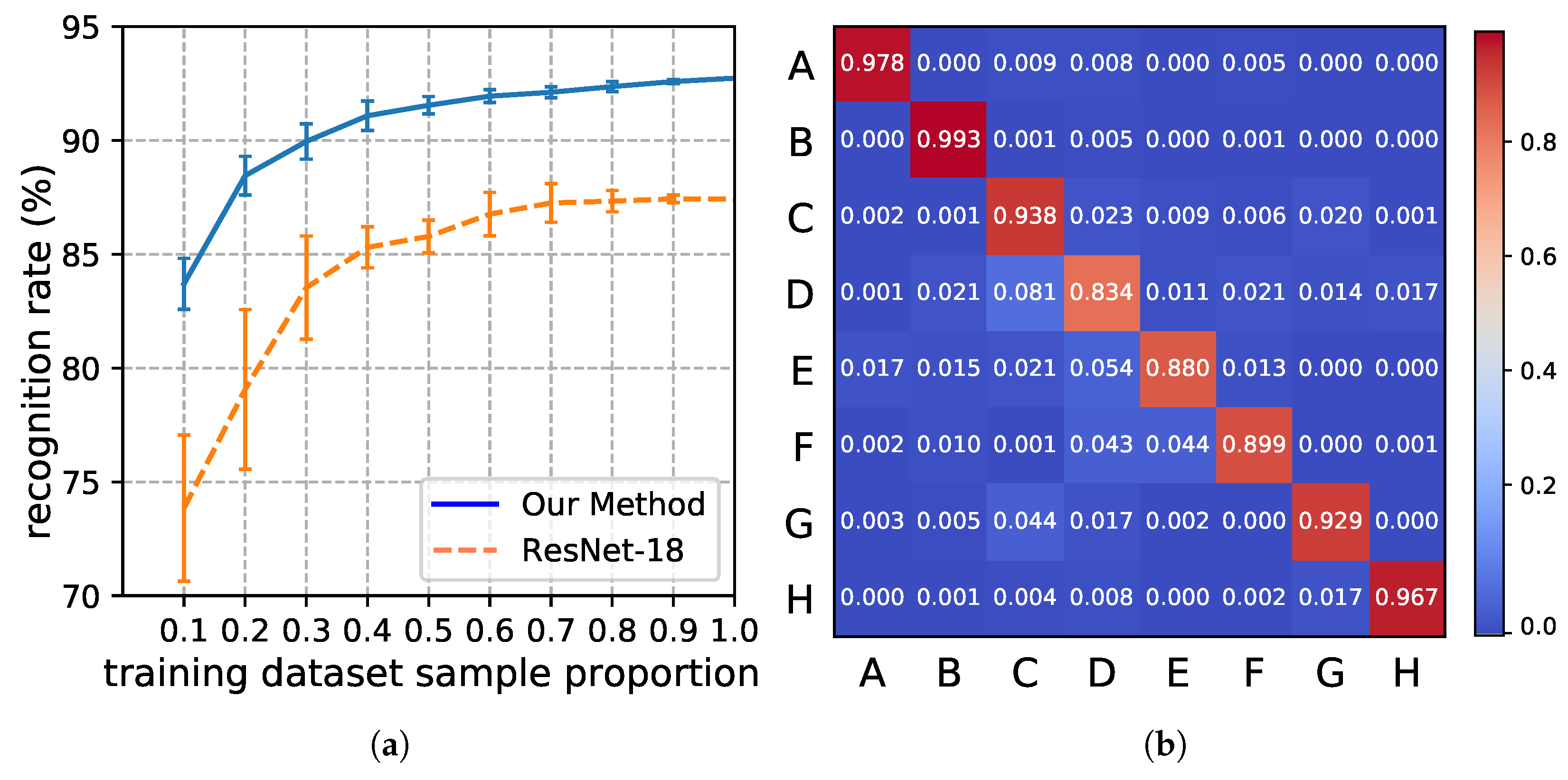
3.4. Aircraft Type Recognition Accuracy Evaluation

We conducted thorough experiments to evaluate our method’s performance in aircraft type recognition. In the experiments, the $\lambda$ of the ROI-weighted loss function was set to 8. We extracted features from the three discriminators, which take images of size $256\times 256$, $128\times 128$, and $64\times 64$ as input, using the ROI feature extraction method. We set the ROI grid sizes of the three discriminators to $5\times 5$, $3\times 3$, and $2\times 2$, respectively. Since the obtained feature contained 19,456 components (which is quite large for SVM), we adopted PCA to process the feature. Through experiments, we found that the first 4096 components contained almost all of the useful information, and its performance was comparable with the entire feature. In the interest of speed and accuracy, we retained 4096 components after the PCA transformation and we trained a linear SVM with $L_2$ regularization based on these features, to identify each aircraft’s type.

3.4.1. Evaluation of the ROI-Weighted Loss Function

To evaluate the effectiveness of the ROI-weighted loss function, we trained GAN models with the same structure by minimizing different loss functions. One of the GANs was trained with the LSGAN loss function [30], while the other GANs were trained with the ROI-weighted loss function using different weight values $\lambda$. We extracted features from those GANs using the same ROI feature extraction method with default parameters, and trained two linear SVM classifiers using the features processed by PCA.

Table 3. Recognition rates (%) of GANs with different loss functions. RWL: ROI-weighted loss function.

Method	Type A	Type B	Type C	Type D	Type E	Type F	Type G	Type H	Mean
LSGAN Loss	95.40	98.10	98.20	83.70	85.70	95.10	83.80	91.50	91.41
RWL $\lambda =2$	93.90	97.60	99.30	88.30	82.60	94.20	83.40	97.40	91.46
RWL $\lambda =4$	93.50	98.10	99.30	84.50	84.20	94.50	83.30	97.60	91.88
RWL $\lambda =8$	93.80	97.80	99.30	88.00	89.90	96.70	83.40	92.90	92.73
RWL $\lambda =10$	93.20	99.30	99.30	82.20	90.80	96.80	81.90	96.40	92.49
RWL $\lambda =16$	93.60	98.70	99.30	88.70	85.60	96.80	81.10	98.10	92.73

shows the results of the GAN models. Benefiting from the recognition framework we designed, our method can achieve 91.41% recognition accuracy on the challenging dataset with only the LSGAN loss function. After adopting the ROI-weighted loss function, the recognition accuracy of our method is further improved. The reason is that the ROI-weighted loss function causes the model to focus on the aircrafts rather than the background, and the features learned by the GAN model are thus more relevant to the aircrafts. Through experiments, we found that, when we set $\lambda =2$, the recognition accuracy is slightly better than the model without using the ROI-weighted loss function. By increasing the value of $\lambda$, the recognition rate increases gradually. However, when the $\lambda >8$, the recognition rate cannot be improved further. If we set $\lambda$ to a larger value, we would need to use a smaller learning rate in the training stage to ensure training stability, which slows down the speed of convergence. Given that, we set $\lambda =8$ in our experiments.

3.4.2. Evaluation of the ROI Feature Extraction Method

To prove the effectiveness of extracting features in the ROI rather than the entire feature map, we conducted experiments with two different feature extraction methods: (1) extracting features using the proposed extraction method on only the ROI; and (2) extracting overall features from the entire feature map with the same operations as Technique (1). In both methods, we extracted features from the three discriminators with grids sizes of $5\times 5$, $3\times 3$, and $2\times 2$ separately. Then, the features were flattened and concatenated to train the linear SVM classifier.

The results are shown in

Table 4. Recognition rate (%) of different feature extraction methods.

Method	Type A	Type B	Type C	Type D	Type E	Type F	Type G	Type H	Mean
Overall Features	91.80	94.90	96.60	83.10	88.00	94.10	66.60	89.60	88.09
ROI Features	93.80	97.80	99.30	88.00	89.90	96.70	83.40	92.90	92.73

. It can be seen that the recognition framework with the overall features achieves 88.09% accuracy on the testing dataset. Although the overall features can distinguish aircrafts of different types, the mixture of background and aircraft information still has a serious influence on the recognition accuracy. On the contrary, the ROI feature extraction method uses the keypoint detection results to locate ROIs and ignore background regions. Therefore, the ROI features abandon redundant information and preserve the most distinctive components. Compared with overall features, ROI features bring about a 4.64% accuracy gain. It is worth noting that the recognition accuracy of each aircraft type is improved by using the ROI features.

3.4.3. Evaluation of the Multi-Scale ROI Features

We compared the three level multi-scale features with other features extracted from different discriminators, including single-scale features and features obtained by combing two different scales. As the results in

Table 5. Recognition rates (%) of different scale features. $F_n$ represents the features extracted from the discriminator which has input image of size $n\times n$, and & represents concatenating features.

Features	Type A	Type B	Type C	Type D	Type E	Type F	Type G	Type H	Mean
$F_{256}$	87.40	93.10	98.30	85.10	81.40	94.20	77.60	92.00	88.64
$F_{128}$	87.30	94.10	95.50	83.30	82.00	96.20	71.30	91.60	87.66
$F_{64}$	74.90	90.00	91.10	64.10	76.30	94.10	53.90	64.10	79.20
$F_{256}$ & $F_{128}$	92.90	96.70	99.00	87.20	88.30	95.00	81.60	91.40	91.51
$F_{256}$ & $F_{64}$	93.00	96.20	98.80	83.00	86.70	95.90	78.40	92.90	90.53
$F_{128}$ & $F_{64}$	87.40	96.70	97.40	82.90	86.70	92.20	74.20	92.20	89.24
$F_{256}$ & $F_{128}$ & $F_{64}$	93.80	97.80	99.30	88.00	89.90	96.70	83.40	92.90	92.73

show, thanks to the recognition framework we designed, the features of single scales can achieve good recognition performance. With the single-scale feature $F_{256}$ or $F_{128}$, the recognition framework achieves more than 87% accuracy. After combining a single scale feature with another scale feature, the recognition accuracy improves significantly, since features from different discriminators contain information of different resolution and they complement each other to achieve better results. It is worth noting that the recognition accuracy decreases substantially with an input size of $64\times 64$, since the aircraft and background information is heavily mixed in the final feature maps of the discriminator. Therefore, we did not downsample the input further. Although the accuracy of $F_{64}$ is less than 80%, when combining $F_{64}$ with $F_{256}$ or $F_{128}$, it increases the accuracy by 1.89% and 1.58%, respectively. Compared with the features of two scales, the feature formed by combing three scales make further progress in the recognition accuracy of all aircraft types. The results show that every single scale feature contains unique information which cannot be replaced by others scale. Multi-scale features can make full use of the information, and thus they have the ability to accurately identify aircrafts of different sizes and resolutions.

3.4.4. Comparison with Other Methods

We conducted experiments to compare our method with other aircraft type recognition methods.

First, we compared our method with several end-to-end methods. In Reference [7], a DBN model was designed for aircraft recognition. We trained and tested the DBN model on our training dataset following the procedure in Reference [7], and the results are shown in

Table 6. Recognition rates (%) of different aircraft type recognition methods. +R represents cases where we make use of the remote sensing image’s resolution to transform the predictions and standard templates to the same scale. DBN, deep belief net.

Method	Type A	Type B	Type C	Type D	Type E	Type F	Type G	Type H	Mean
AlexNet [8]	75.60	97.80	95.90	70.40	69.80	98.00	64.30	91.00	82.85
VGG-16 [9]	82.30	98.40	89.80	87.30	67.50	96.90	74.60	90.20	85.88
ResNet-18 [11]	86.10	99.30	96.60	82.60	69.80	99.70	79.20	84.60	87.24
DBN [7]	83.40	93.60	92.60	80.40	68.80	93.60	78.50	85.64	84.56
Method in [16]	91.70	80.70	91.10	79.50	17.40	47.80	30.10	72.60	63.86
Method in [16] +R	99.70	88.00	96.10	99.60	99.90	88.60	99.90	75.70	93.44
Our Keypoints	92.60	98.00	87.50	97.50	34.10	97.10	43.00	71.10	77.61
Our Keypoints +R	99.70	99.50	92.00	99.10	99.40	99.80	99.60	76.20	95.66
Proposed Method	93.80	97.80	99.30	88.00	89.90	96.70	83.40	92.90	92.73

. Limited by the shallow network structure of the DBN, the features learned by the model lack robustness and representation ability. Therefore, the accuracy of the DBN method is lower than our method by more than 7%. Additionally, we trained some typical CNN models, including AlexNet [8], VGG-16 [9], and ResNet-18 [11], and compared their performance with our method. As the results in Table 6 show, although these methods can achieve good results on large classification dataset such as ImageNet [12] and MSCOCO [13], their performance is worse than our method on the aircraft recognition dataset. On the one hand, the performance of these methods relies on the quantity of labeled data. Limited by the amount of labeled aircraft samples in remote sensing images, these methods suffer from overfitting. On the other hand, these CNN models tend to learn global semantic features to classify different objects. However, since some aircrafts only occupy small regions of images, aircraft information is submerged in background information and ignored by these CNN models. Different from CNN models, our method adopts GAN to learn features from large amounts of data without type labels, which complements the shortage of labeled data. Besides, since our method extracts features from ROIs directly, the redundant background information is effectively eliminated. Therefore, our method outperforms the end-to-end models by more than 5%.

We also compared our method with the state-of-the-art template matching method in Reference [16]. Following the procedure described there, we trained the segmentation network and keypoint detection network on our training dataset, and then matched their predictions with the standard templates. Because the method requires resolution information to make the predictions and standard templates under the same scale condition, we made use of remote sensing image resolution to conduct the template matching experiments, as in Reference [16], on our testing dataset. The results are shown in Table 6, marked as Method in [16] +R. Since this method makes use of both scale and shape characteristics to distinguish aircrafts of different types, it can achieve 93.44% accuracy on the testing dataset. To evaluate this method’s performance without resolution, we resized all of their predictions and standard templates to $256\times 256$ and adopted the template matching method for recognition. The results are shown in Table 6, marked as Method in [16]. Without using resolution information, this method only achieves 63.86% accuracy.

In this paper, we propose a new method for aircraft keypoint detection which obtains more precise keypoints than the method in Reference [16]. Therefore, we also conducted experiments using the same procedure as in Reference [16], but replacing the keypoint detection module with ours. The results in Table 6, marked as Our keypoints +R, show that benefiting from the improvement of keypoints’ precision, the recognition rates are advanced substantially. However, without using resolution, the accuracy of this method is still less than 80%, marked as Our keypoints. These experiments prove that the performance of the template matching method in Reference [16] relies heavily on resolution information, which confines its practicability in actual applications. Without resolution information, the method loses important scale characteristics and it can only use shape characteristics to distinguish aircrafts of different types. On the contrary, the recognition framework we designed does not require resolution information, and is able to learn representative features from a large amount of aircraft samples. The multi-scale ROI features ensure that our method can deal with aircrafts of different shapes and scales effectively.

As we state above, one of the advantages of our method is that it can achieve a high recognition rate with only a small labeled training dataset. Therefore, we designed an experiment to evaluate the dependence of our method on the quantity of training data. Specifically, we randomly took samples from the training dataset in a certain proportion from 0.1 to 1 with a step of 0.1, and built some sub-datasets for training. Then, we used the sub-datasets to train different SVM classifiers and recognized aircrafts following the procedure we proposed. We built five sub-datasets for every proportion. Then, we calculated the mean value and the standard deviation of recognition rates. Additionally, we repeated the procedure using ResNet-18 as the baseline method. The results are shown in Figure 8a. The mean values of the proportions are drawn as lines, and values of error bars are calculated by:

$$\mathrm{value}\mathrm{of}\mathrm{error}\mathrm{bar}=\mathrm{mean}\mathrm{value}\pm \mathrm{standard}\mathrm{deviation}.$$

(4)

It is obvious that our method achieves a high recognition rate with small standard deviations using only a small training dataset. On the other hand, with the decrease of sampling proportion, the performance of ResNet-18 was greatly reduced and the standard deviations were much larger than our method’s. This indicates that our method is less dependent on the quantity of training samples compared with convolutional neural networks. Therefore, our method is more suitable for dealing with aircraft type recognition on the condition that there are large amounts of data but only a few samples are labeled with type information.

Finally, we report the confusion matrix of our method in Figure 8b, which shows our method’s performance on each type directly. The proposed method can effectively distinguish different types of aircrafts.

4. Discussion

In remote sensing image interpretation, there is a large amount of data available, but only some of the data are labeled with type information. Although some template matching methods can handle this situation, strict prerequisites make it difficult for them to be widely applied in practice. End-to-end methods can usually achieve good recognition rates, but they demand a large amount of labeled samples. However, limited by the quantity of labeled data in remote sensing images, they suffer from bad generation performance. It is obvious that the amount of labeled data has become an important factor blocking end-to-end classification method development in remote sensing image interpretation. Considering that, we designed a new framework to make full use of large amounts of unlabeled data. One of the important parts of this framework is the GAN model, which is used to learn features from images without supervision. Some examples of generated samples are shown in Figure 9. It can be seen that the generated samples have high quality and diversity, which provide abundant data for discriminators to learn strong features. The high performance of the GAN builds a solid foundation for our entire method.

Additionally, all of the previous methods process entire images directly regardless of the scales of the targets in the images. Large amounts of background features mislead the model and cause it to make incorrect classifications. Given that, we designed the ROI-weighted loss function and ROI feature extraction method to learn features from exactly where the targets are. A great deal of useless information is removed and the features are further refined. The experiments we conducted revealed the effectiveness of our method.

In our aircraft type recognition framework, we use keypoints to generate aircraft masks and obtain ROIs for the ROI-weighted loss function and the ROI feature extraction methods. Therefore, the performance of the keypoint detection network has a strong influence on our framework’s recognition accuracy. To evaluate our keypoints detection network’s impact on the recognition task, we conducted experiments with our method’s keypoint predictions and keypoint ground truths, respectively. As the results in

Table 7. Recognition rates (%) with or without keypoint ground truths.

Method	Type A	Type B	Type C	Type D	Type E	Type F	Type G	Type H	Mean
Ground Truth	93.60	98.50	99.40	89.40	91.00	96.60	84.30	96.50	93.65
Predicted Result	93.80	97.80	99.30	88.00	89.90	96.70	83.40	92.90	92.73

show, although our keypoint detection method outperforms the state-of-the-art method [16], it still decreases the recognition rate by almost 1% compared with the keypoint ground truths. Thus, the recognition rate of our framework can be further increased by using more accurate keypoint detection results. In the future, we will continue studying the keypoint detection model to improve its performance.

5. Conclusions

In this paper, we present an aircraft type recognition framework based on a conditional GAN. First, a new aircraft keypoint detection method was carefully designed to predict the eight keypoint positions precisely. The keypoint detection results provided an accurate mask and ROI information for the GAN and feature extraction methods. Then, a conditional GAN with an ROI-weighted loss function was proposed to learn features from a large dataset without type labels. Finally, we designed an ROI feature extraction method to extract multi-scale features in the regions of targets and eliminate the effects of complex background information. Experiments demonstrated that the proposed framework could effectively extract robust and distinctive features. Based on the features, our method was able to identify aircrafts of different types and scales, and it achieved good recognition performance on a challenging dataset.

Although our method is effective in aircraft recognition, it can still be improved further. In the future, we will explore how to build an unsupervised classification method to remove the need for data labeled with type information.

References

1. Hsieh, J.W.; Chen, J.M.; Chuang, C.H.; Fan, K.C. Aircraft type recognition in satellite images. IEE Proc. Vis. Image Signal Process. 2005, 152, 307. [Google Scholar] [CrossRef]
2. Liu, G.; Sun, X.; Fu, K.; Wang, H. Aircraft Recognition in High-Resolution Satellite Images Using Coarse-to-Fine Shape Prior. IEEE Geosci. Remote Sens. Lett. 2013, 10, 573–577. [Google Scholar] [CrossRef]
3. Xu, C.; Duan, H. Artificial bee colony (ABC) optimized edge potential function (EPF) approach to target recognition for low-altitude aircraft. Pattern Recognit. Lett. 2010, 31, 1759–1772. [Google Scholar] [CrossRef]
4. Wang, D.; He, X.; Zhonghui, W.; Yu, H. A method of aircraft image target recognition based on modified PCA features and SVM. In Proceedings of the 2009 9th International Conference on Electronic Measurement & Instruments, Beijing, China, 16–19 August 2009. [Google Scholar] [CrossRef]
5. Fang, Z.; Yao, G.; Zhang, Y. Target recognition of aircraft based on moment invariants and BP neural network. In Proceedings of the World Automation Congress, Puerto Vallarta, Mexico, 24–28 June 2012; pp. 1–5. [Google Scholar]
6. Wu, H.; Li, D.; Wang, H.; Liu, Y.; Sun, X. Research on Aircraft Object Recognition Model Based on Neural Networks. In Proceedings of the 2012 International Conference on Computer Science and Electronics Engineering, Hangzhou, China, 23–25 March 2012; Volume 1, pp. 160–163. [Google Scholar] [CrossRef]
7. Diao, W.; Sun, X.; Dou, F.; Yan, M.; Wang, H.; Fu, K. Object recognition in remote sensing images using sparse deep belief networks. Remote Sens. Lett. 2015, 6, 745–754. [Google Scholar] [CrossRef]
8. Krizhevsky, A.; Sutskever, I.; Hinton, G.E. ImageNet classification with deep convolutional neural networks. Commun. ACM 2017, 60, 84–90. [Google Scholar] [CrossRef] [Green Version]
9. Simonyan, K.; Zisserman, A. Very Deep Convolutional Networks for Large-Scale Image Recognition. arXiv, 2014; arXiv:1409.1556. [Google Scholar]
10. Szegedy, C.; Liu, W.; Jia, Y.; Sermanet, P.; Reed, S.; Anguelov, D.; Erhan, D.; Vanhoucke, V.; Rabinovich, A. Going deeper with convolutions. In Proceedings of the 2015 IEEE Conference on Computer Vision and Pattern Recognition (CVPR), Boston, MA, USA, 7–12 June 2015; pp. 1–9. [Google Scholar] [CrossRef]
11. He, K.; Zhang, X.; Ren, S.; Sun, J. Deep Residual Learning for Image Recognition. In Proceedings of the 2016 IEEE Conference on Computer Vision and Pattern Recognition (CVPR), Las Vegas, NV, USA, 26 June–1 July 2016; pp. 770–778. [Google Scholar] [CrossRef]
12. Deng, J.; Dong, W.; Socher, R.; Li, L.J.; Li, K.; Li, F.-F. ImageNet: A large-scale hierarchical image database. In Proceedings of the 2009 IEEE Conference on Computer Vision and Pattern Recognition, Miami, FL, USA, 20–25 June 2009; pp. 248–255. [Google Scholar] [CrossRef]
13. Lin, T.Y.; Maire, M.; Belongie, S.; Hays, J.; Perona, P.; Ramanan, D.; Dollár, P.; Zitnick, C.L. Microsoft COCO: Common Objects in Context. In Computer Vision—ECCV 2014; Fleet, D., Pajdla, T., Schiele, B., Tuytelaars, T., Eds.; Springer International Publishing: Cham, Switzerland, 2014; pp. 740–755. [Google Scholar]
14. Wu, Q.; Sun, H.; Sun, X.; Zhang, D.; Fu, K.; Wang, H. Aircraft Recognition in High-Resolution Optical Satellite Remote Sensing Images. IEEE Geosci. Remote Sens. Lett. 2015, 12, 112–116. [Google Scholar] [CrossRef]
15. Zhao, A.; Fu, K.; Wang, S.; Zuo, J.; Zhang, Y.; Hu, Y.; Wang, H. Aircraft Recognition Based on Landmark Detection in Remote Sensing Images. IEEE Geosci. Remote Sens. Lett. 2017, 14, 1413–1417. [Google Scholar] [CrossRef]
16. Zuo, J.; Xu, G.; Fu, K.; Sun, X.; Sun, H. Aircraft Type Recognition Based on Segmentation With Deep Convolutional Neural Networks. IEEE Geosci. Remote Sens. Lett. 2018, 15, 282–286. [Google Scholar] [CrossRef]
17. Goodfellow, I.J.; Pouget-Abadie, J.; Mirza, M.; Xu, B.; Warde-Farley, D.; Ozair, S.; Courville, A.; Bengio, Y. Generative Adversarial Nets. In Proceedings of the 27th International Conference on Neural Information Processing Systems—Volume 2, NIPS’14; MIT Press: Cambridge, MA, USA, 2014; pp. 2672–2680. [Google Scholar]
18. Radford, A.; Metz, L.; Chintala, S. Unsupervised Representation Learning with Deep Convolutional Generative Adversarial Networks. arXiv, 2015; arXiv:1511.06434. [Google Scholar]
19. Isola, P.; Zhu, J.Y.; Zhou, T.; Efros, A.A. Image-to-Image Translation with Conditional Adversarial Networks. In Proceedings of the 2017 IEEE Conference on Computer Vision and Pattern Recognition (CVPR), Honolulu, HI, USA, 21–26 July 2017; pp. 5967–5976. [Google Scholar] [CrossRef]
20. Wang, T.C.; Liu, M.Y.; Zhu, J.Y.; Tao, A.; Kautz, J.; Catanzaro, B. High-Resolution Image Synthesis and Semantic Manipulation with Conditional GANs. arXiv, 2017; arXiv:1711.11585. [Google Scholar]
21. Corres, C. Support vector networks. Mach. Learn. 1995, 20, 273–297. [Google Scholar]
22. Newell, A.; Yang, K.; Deng, J. Stacked Hourglass Networks for Human Pose Estimation. In Computer Vision—ECCV 2016; Leibe, B., Matas, J., Sebe, N., Welling, M., Eds.; Springer International Publishing: Cham, Switzerland, 2016; pp. 483–499. [Google Scholar]
23. Mirza, M.; Osindero, S. Conditional Generative Adversarial Nets. arXiv, 2014; arXiv:1411.1784. [Google Scholar]
24. Salimans, T.; Goodfellow, I.; Zaremba, W.; Cheung, V.; Radford, A.; Chen, X.; Chen, X. Improved Techniques for Training GANs. In Advances in Neural Information Processing Systems 29; Lee, D.D., Sugiyama, M., Luxburg, U.V., Guyon, I., Garnett, R., Eds.; Curran Associates, Inc.: Red Hook, NY, USA, 2016; pp. 2234–2242. [Google Scholar]
25. Arjovsky, M.; Chintala, S.; Bottou, L. Wasserstein GAN. arXiv, 2017; arXiv:stat.ML/1701.07875. [Google Scholar]
26. Fergus, R.; Fergus, R.; Fergus, R.; Fergus, R. Deep generative image models using a Laplacian pyramid of adversarial networks. In Proceedings of the International Conference on Neural Information Processing Systems, Montréal, QC, Canada, 7–12 December 2015; pp. 1486–1494. [Google Scholar]
27. Huang, X.; Li, Y.; Poursaeed, O.; Hopcroft, J.; Belongie, S. Stacked Generative Adversarial Networks. In Proceedings of the 2017 Conference on Computer Vision and Pattern Recognition, Honolulu, HI, USA, 21–26 July 2017. pp. 1866–1875.
28. Chen, Q.; Koltun, V. Photographic Image Synthesis with Cascaded Refinement Networks. arXiv, 2017; arXiv:1707.09405. [Google Scholar] [Green Version]
29. Zhang, H.; Xu, T.; Li, H. StackGAN: Text to Photo-Realistic Image Synthesis with Stacked Generative Adversarial Networks. arXiv, 2017; arXiv:1612.03242. [Google Scholar] [Green Version]
30. Mao, X.; Li, Q.; Xie, H.; Lau, R.Y.K.; Wang, Z.; Smolley, S.P. Least Squares Generative Adversarial Networks. In Proceedings of the IEEE International Conference on Computer Vision (ICCV), Venice, Italy, 22–29 October 2017; pp. 2813–2821. [Google Scholar] [CrossRef]
31. Kingma, D.P.; Ba, J. Adam: A Method for Stochastic Optimization. arXiv, 2014; arXiv:1412.6980. [Google Scholar]
32. Pedregosa, F.; Varoquaux, G.; Gramfort, A.; Michel, V.; Thirion, B.; Grisel, O.; Blondel, M.; Prettenhofer, P.; Weiss, R.; Dubourg, V.; et al. Scikit-learn: Machine Learning in Python. J. Mach. Learn. Res. 2011, 12, 2825–2830. [Google Scholar]
Figure 1. The framework of our proposed model training and recognition procedures. The boxes with solid lines are algorithm modules, while the boxes with dotted lines are the modules’ outputs. (a) Training of the generative adversarial network (GAN) model. The generator takes aircraft masks as input, which are generated based on keypoints, and the discriminators learn features by distinguishing generated samples from real images. Type labels are not used in the training procedure. (b) Outline of the recognition procedure. Abbreviations: ROI, region of interest; SVM, support vector machine; PCA, principal component analysis.
Remotesensing 10 01123 g001
Figure 2. Examples of the typical images in the dataset. (Top) Eight types of aircrafts labeled with keypoints (red points)—nose, tail, two wingtips, and the four joints of the wings and the fuselage. (Bottom) Polygon masks of the same aircrafts generated based on the keypoints. Different types of aircrafts are indicated with letters from A to H.
Remotesensing 10 01123 g002
Figure 3. An example of the keypoint heat map ground truths of our method. (a) Image; (b) Nose heat map; (c) Tail heat map; (d) Wingtips heat map; (e) Top Joints heat map; (f) Bottom Joints heat map.
Remotesensing 10 01123 g003
Figure 4. Architecture of the generator used in this paper. The generator contains two networks: G 1 and G 2 . G 2 is decomposed into two sub-networks: G 2 F and G 2 B .
Remotesensing 10 01123 g004
Figure 5. ROI weighted loss function. The ROI is the minimum outer rectangle, encompassing the keypoints. The light blue grid values of the ROI weight map are set to 1, while the deep blue grid values are set to λ . Additionally, the parameters of the discriminator are annotated, where s represents the size of stride and p represents the size of padding. MSE represents the mean square error.
Remotesensing 10 01123 g005
Figure 6. ROI feature extraction method. The ROIs are located by keypoints and mapped to the last feature map according the scale ratio. After that, the features are extracted from the ROIs by the method we designed.
Remotesensing 10 01123 g006
Figure 7. Examples of aircraft keypoint detection results on a testing dataset: (top) the results of our method; and (bottom) the results of the original hourglass model [22]. The noses are annotated with yellow dots and the tails are annotated with green dots. All of the left keypoints are annotated with blue dots, while all of the right keypoints are annotated with red dots.
Remotesensing 10 01123 g007
Figure 8. (a) The recognition rates of models trained on different proportions of the dataset with error bars. The solid blue line is the result of our aircraft type recognition method, while the dash orange line is the result of ResNet-18 model. (b) The confusion matrix of our method. The closer the color is to the red, the higher is the recognition rate, while the closer the color is to the blue, the lower is the recognition rate.
Remotesensing 10 01123 g008
Figure 9. Examples of generated samples on the testing dataset: (top) masks of aircrafts; (middle) real images; and (bottom) generated samples.
Remotesensing 10 01123 g009