A Compensation Method for Airborne SAR with Varying Accelerated Motion Error

Abstract

Motion error is one of the most serious problems in airborne synthetic aperture radar (SAR) data processing. For a smoothly distributing backscatter scene or a seriously speed-varying velocity platform, the autofocusing performances of conventional algorithms, e.g., map-drift (MD) or phase gradient autofocus (PGA) are limited by their estimators. In this paper, combining the trajectories measured by global position system (GPS) and inertial navigation system (INS), we propose a novel error compensation method for varying accelerated airborne SAR based on the best linear unbiased estimation (BLUE). The proposed compensating method is particularly intended for varying acceleration SAR or homogeneous backscatter scenes, the processing procedures and computational cost of which are much simpler and lower than those of MD and PGA algorithms.

1. Introduction

Space-borne and airborne synthetic aperture radar (SAR) can work well day-and-night and weather-independently [1,2,3]. With high resolution image production, SAR is widely applied in remote sensing applications, e.g., Earth observation, marine surveillance, earthquake and volcano detection, interferometry, and differential interferometry. However, image quality of SAR signal processors greatly depends on the smoothness of platform movement. The orbit of space-borne SAR is relatively stable in vacuum-like environments while, with the influence of atmospheric turbulence, the trajectory of airborne SAR fluctuates seriously around a nominal straight line in the cross-velocity direction. Achieving a high-quality SAR image from the systems with platform trajectory error has been a hot topic in airborne SAR configurations.

SAR transmits a wide bandwidth chirp signal to achieve high resolution along the range direction, but azimuth resolution depends on the antenna size along the azimuth direction, and usually requires intensive coherent data processing (focusing or pulse compression) to synthesize an antenna array several times larger than the actual illuminating antenna [4]. Motion error results in the deterioration of the space coherent relativity and further influences the focusing along the azimuth dimension of airborne SAR images. It is important to find a robust and effective motion error compensation (MOCO) method to achieve high-quality airborne SAR images. High-quality SAR images are fundamental inputs for extensive SAR applications, including agriculture or vegetation surveys from fully polarized data [5]. On the premise of obtaining the trajectory of the antenna phase center (APC), the back projection (BP) algorithm is the most precise imaging method. However, it also has the largest computational cost, and most Fast Fourier Transform (FFT)-based focusing methods, which can obviously reduce computational cost, are based on uniform sampling in the range and azimuth dimensions, while in airborne SAR missions, motion error will cause the APC deviation from the ideal position, and essentially leads to non-uniform spatial sampling. Based on global position system (GPS) or inertial navigation system (INS) data, a two-step algorithm [6] is proposed to compensate the motion errors along pitch and yaw. Furthermore, autofocusing algorithms are introduced to correct the velocity variance, e.g., map-drift (MD) algorithm and the phase gradient autofocus (PGA) algorithm. Classical MD [7] or phase curve autofocus algorithms [8] work well with second-order motion error, while PGA [9,10] is more sensitive to the second and higher order motion error, which primarily introduced in spotlight SAR autofocusing. However, in strip-map or sliding spotlight SAR processing, the echo data needs to be divided into sub-apertures to apply PGA algorithms to correct motion error, which will lead to phase discontinuities along the azimuth direction. This restricts the phase-depending applications, e.g., interferometry and differential interferometry.

MD and PGA algorithms have advantages in extracting the motion error from raw data without the other auxiliary information. However, current autofocus algorithms, including MD and PGA algorithms, cannot compensate for the intensive velocity variance in the aperture scope. In addition, autofocusing performances of MD and PGA algorithms seriously degrade in homogeneous backscatters scenes, such as grassland and sea, because the estimation accuracies rely heavily on the strong backscatter, which limits the application scopes of the current autofocus algorithm. In this paper, we proposes a new compensation method based on the best linear unbiased estimation (BLUE) to correct varying accelerated motion error using GPS- and INS-measured trajectories. The proposed algorithm essentially adopts the BLUE algorithm, combining with the information of its azimuth power spectrum and trajectory data, to reconstruct the uniform sampling SAR data. Its computational cost is lower than MD and PGA algorithms, which provides significant improvement for marked velocity varying SAR data or homogeneous backscatter scenes.

The structure of this paper is as follows: Section 2 introduces BLUE algorithm details and the processing blocks. Section 3 presents simulation and real data procession results and compares autofocusing performances of different algorithms. Section 4 discusses the influences of residual and positioning errors to the proposed algorithm. Finally, Section 5 summarizes and concludes the paper.

2. Best Linear Unbiased Estimation

2.1. Why BLUE Works

The geometry of airborne SAR with motion error is given in Figure 1. The dashed line and solid curve line represent ideal and actual trajectories, respectively. $\eta$ is slow time. The platform flight direction is along Y axis with forward velocity $V_r\left(\eta \right)$, A is the radar position on an ideal trajectory at ${\eta }_m$ with coordinates $\left(0,y\left({\eta }_m\right),H\right)$. $H$ is the height of position $A$; $d\left(\Delta x\left({\eta }_m\right),\Delta y\left({\eta }_m\right),\Delta z\left({\eta }_m\right)\right)$ is the motion error vector between the ideal and actual trajectories. ${\eta }_m$ is the m-th sampling moment along azimuth. $P$ is a target in the illuminated region with coordinate $\left(X_n,Y_n,Z_n\right)$, and θ is the instantaneous squint angle between radar and target $P$. Actually, the antenna of airborne SAR is mounted on a stable board precisely controlled by INS, which guarantees that the beam can steadily illuminate the area of interest.

Assume that the position errors in the X axis, $\Delta \mathbf{X}\left(\Delta \mathbf{X}=\left\{\Delta x\left({\eta }_m\right),m=0,1,\dots ,N\right\}\right)$, and in the Z axis, $\Delta \mathbf{Z}\left(\Delta \mathbf{Z}=\left\{\Delta z\left({\eta }_m\right),m=0,1,\dots ,N\right\}\right)$, are compensated by the data measured by INS and GPS, where m is the azimuth sampling index. After initial motion compensation (MOCO) by $\Delta \mathbf{x}$ and $\Delta \mathbf{z}$, residual position error $\Delta \mathbf{Y}\left(\Delta \mathbf{Y}=\left\{\Delta y\left({\eta }_m\right),m=0,1,\dots ,N\right\}\right)$ can be considered as a result of non-uniform sampling along the azimuth direction, because the forward velocity $V_r\left(\eta \right)$ is time-variant. Figure 2 shows the sampling along the azimuth direction.

In Figure 2, the horizontal direction is azimuth. $y_a\left({\eta }_k\right)$ and $y_i\left({\eta }_k\right)$ represent the actual and ideal sample positions along azimuth dimension at the moment ${\eta }_k\left(k=0,1,2,\dots ,N\right)$, respectively. $s\left(y_a\left({\eta }_k\right)\right)$ and $s\left(y_i\left({\eta }_k\right)\right)$ represent the recorded echo at the actual and ideal sample positions, respectively.

Considering the geometry in Figure 2:

$$\begin{array}{l}{y}_a\left({\eta }_m\right)=y\left({\eta }_m\right)+\Delta y\left({\eta }_m\right)\\ y_i\left({\eta }_m\right)=y\left({\eta }_m\right)\end{array}$$

(1)

Assume that:

$$\begin{array}{l}{\mathbf{S}}_0=\left[s\left(y_a\left({\eta }_0\right)\right),s\left(y_a\left({\eta }_1\right)\right),\cdots ,s\left(y_a\left({\eta }_N\right)\right)\right]\\ {\mathbf{S}}_1=\left[s\left(y_i\left({\eta }_0\right)\right),s\left(y_i\left({\eta }_1\right)\right),\cdots ,s\left(y_i\left({\eta }_N\right)\right)\right]\end{array}$$

(2)

where ${\mathbf{S}}_0$ are the observation samples; therefore combining Figure 2, Equations (1) and (2), we can get that the key procedure is how to recover ${\mathbf{S}}_1$ from ${\mathbf{S}}_0$. For airborne SAR, the turbulent flow is unpredicted. Hence, the signal along the azimuth dimension can be treated as a random sampling process in space. Meanwhile, the antenna azimuth pattern results in that the sampling process is band-limited. This band-limited signal has its power spectrum density (PSD). If the PSD is known, BLUE can accurately estimate the random process signal at the desired time or space position [11].

Statistical property of the raw azimuth signal is used in this paper to recover the uniform sample signal from the non-uniform ones. SAR azimuth signal can be considered as a random process and the deduced blocks for BLUE are discussed in [11]. This paper will not explain again. Readers can get the details from [11]. The key procedure of BLUE is to calculate the signal PSD.

In most real SAR systems, the azimuth pattern is a Sinc function. In this paper, neglecting the beam expanded effect, we assume the antenna azimuth pattern is a Sinc function and it can be expressed as [12]:

$$F\left(\theta \right)=\sin \mathrm{c}\left[\pi \frac{L_a}{\lambda }\sin \left(\theta \right)\right]$$

(3)

where $L_a$ is the azimuth size of the antenna; $\lambda$ is the wavelength of the signal transmitted by the radar. As shown in Figure 1, $\theta$ is the instantaneous angle between the flight direction vector and the vector of instantaneous slant range. The relationship between the Doppler $f$ and the angle $\theta$ is as follows [13]:

$$f=\frac{2V_r}{\lambda }\sin \left(\theta \right)$$

(4)

Combining Equations (3) and (4), we can obtain the antenna signal spectrum:

$$U\left(f\right)=\sin \mathrm{c}\left(\pi \frac{L_a}{2V_r}f\right)$$

(5)

Since the signal is a two-way radar echo, the azimuth signal spectrum can be expressed as:

$$S\left(f\right)=U^2\left(f\right)={\sin \mathrm{c}}^2\left(\pi \frac{L_a}{2V_r}f\right)$$

(6)

Hence, the azimuth signal PSD is given as follows:

$$P_s\left(f\right)=S\left(f\right)S^{*}\left(f\right)={\sin \mathrm{c}}^4\left(\pi \frac{L_a}{2V_r}f\right)$$

(7)

From the perspective of auto-correlation, the signal PSD is the Fourier transform of its auto-correlation coefficients. Hence, the auto-correlation coefficients of the azimuth signal can be expressed as:

$$\begin{array}{cc}\hfill R_s\left(\xi \right)& =\frac{E\left[s^{*}\left(\eta \right)s\left(\eta +\xi \right)\right]}{E\left[{\left|s\left(\eta \right)\right|}^2\right]}={\displaystyle \underset{-\infty }{\overset{+\infty }{\int }}{P}_s\left(f\right)}\exp \left[j2\pi f\xi \right]\mathrm{d}f\hfill \\ & =\frac{1}{6\sqrt{2}{\pi }^{\frac{7}{2}}{t}_0^4}\left[\begin{array}{l}6{\xi }^3\mathrm{sign}\left(\xi \right)+{\left(\xi -2\pi t_0\right)}^3\mathrm{sign}\left(\xi -2\pi t_0\right)-4{\left(\xi -\pi t_0\right)}^3\mathrm{sign}\left(\xi -\pi t_0\right)\\ -4{\left(\xi +\pi t_0\right)}^3\mathrm{sign}\left(\xi +\pi t_0\right)+{\left(\xi +2\pi t_0\right)}^3\mathrm{sign}\left(\xi +2\pi t_0\right)\end{array}\right]\hfill \end{array}$$

(8)

where the coefficient $t_0$ is equal to $L_a/V_r$; $\mathrm{sign}(·)$ is the sign function; $\xi$ is the time or space variables of auto-correlation coefficients. The details of derivation are given in the Appendix. The constraint, attached to Equation (8), is given as follow:

$$R_s\left(\xi \right)=0,\left|\xi \right|>t_0$$

(9)

and $V_{opt}$ is the optimized velocity, which can be calculated from the trajectory data as the following equation:

$$V_{opt}=\mathrm{Mode}\left[\frac{\mathrm{d}{y}_a\left(\eta \right)}{\mathrm{d}\eta }\right]$$

(10)

where $\mathrm{Mode}[·]$ is the most often repeated value in the dataset. In a real linear airborne SAR system, the platform maintains a constant velocity region by its motion control device. Hence, we choose the most often repeated value as the optimal velocity.

${\eta }_{\mathrm{non}-\mathrm{uni}}$ and ${\eta }_{\mathrm{uni}}$ represent sample moments of trajectories with motion error and ideal ones, respectively. They can be considered as non-uniform and uniform sample moments:

$$\begin{array}{l}{\eta }_{\mathrm{non}-\mathrm{uni}}=\frac{y_a\left(\eta \right)}{V_{opt}}\\ {\eta }_{\mathrm{uni}}=\frac{y\left(\eta \right)}{V_{opt}}\end{array}$$

(11)

Then the best linear unbiased estimator is given as:

$$\widehat{s}\left({\eta }_{\mathrm{uni}}\right)={\mathbf{r}}^{\mathrm{T}}{\mathbf{H}}^{-1}\mathbf{s}$$

(12)

where $\mathbf{s}$ is a column vector including K values $s\left({\eta }_{\mathrm{non}-\mathrm{uni}}\right)$ ($k=1,2,\dots ,K$), which meets the following constraint:

$$\left|{\eta }_{\mathrm{uni}}-{\eta }_{\mathrm{non}-\mathrm{uni}}\right|<t_0$$

(13)

$\mathbf{r}$ is also a column vector and its elements can be expressed as:

$$r=R_s\left({\eta }_{\mathrm{uni}}-{\eta }_{\mathrm{non}-\mathrm{uni}}\right),k=1,2,\cdots ,K$$

(14)

The elements of the matrix $\mathbf{H}$ are given as follows:

$$h_{j,k}=R_s\left({\eta }_{\mathrm{non}-\mathrm{uni},j}-{\eta }_{\mathrm{uni},k}\right),j=1,2,\cdots ,K,k=1,2,\cdots ,K$$

(15)

Furthermore, the variance of the estimation is given by [10]:

$$E\left[{\left|{\widehat{s}}_{\mathrm{uniform}}\left({\eta }_{\mathrm{uni}}\right)-s_{\mathrm{uniform}}\left({\eta }_{\mathrm{uni}}\right)\right|}^2\right]/E\left[{\left|s_{\mathrm{uniform}}\left({\eta }_{\mathrm{uni}}\right)\right|}^2\right]=1-{\mathbf{r}}^{\mathrm{T}}{\mathbf{H}}^{-1}\mathbf{r}$$

(16)

From Equation (12), the BLUE algorithm can recover the non-uniform signal to a uniform sampling grid. It means that the BLUE algorithm has the capability of correcting the varying accelerated motion error along azimuth dimension. Combined with Equations (8), (14), and (12), we can obtain that the best linear unbiased estimator only uses the information of azimuth signal PSD and sampling position to recover the effective uniform sampling signal. It means that the estimation result is independent of any scene (homogeneous or non-homogeneous scatters).

2.2. Blocks of Proposed Algorithm

Figure 3 depicts the procedures of compensation method for SAR data processing, and the steps are as follows:

Step 1: From the trajectory-like INS data, we can extract the motion error $\left\{\Delta \mathbf{X},\Delta \mathbf{Z}\right\}$ of the X and Z axes. Then, combined with the motion error data $\left\{\Delta \mathbf{X},\Delta \mathbf{Z}\right\}$, the two-step algorithm is applied into the correction of the MOCO for the X and Z axes. In this step the motion errors along the pitch and yaw directions can be mostly suppressed by the two-step algorithm.

Step 2: Extract the $y_a\left(\eta \right)$ and $V_{opt}$ from the INS data. We can obtain the vectors of auto-coefficients $\mathbf{r}$ and $\mathbf{H}$ by referring to Equations (11), (14), and (15).

Step 3: Combining the vectors $\left\{\mathbf{r},\mathbf{H}\right\}$ calculated from Step 2 and the SAR data $s\left({\eta }_{\mathrm{non}-\mathrm{uni}}\right)$ processed after the two-step algorithm, we can estimate the uniform sampled signal $\widehat{s}\left({\eta }_{\mathrm{uni}}\right)$ by using Equation (12);

Step 4: We can obtain the effective uniform sampled signal by the same processing from Step 1–Step 3 for the echo. Then, we process the estimated data by the traditional SAR processor, such as chirp scaling (CS), range Doppler (RD), and $\omega -k$ algorithms, to obtain the focusing data.

3. Experiment Results and Discussion

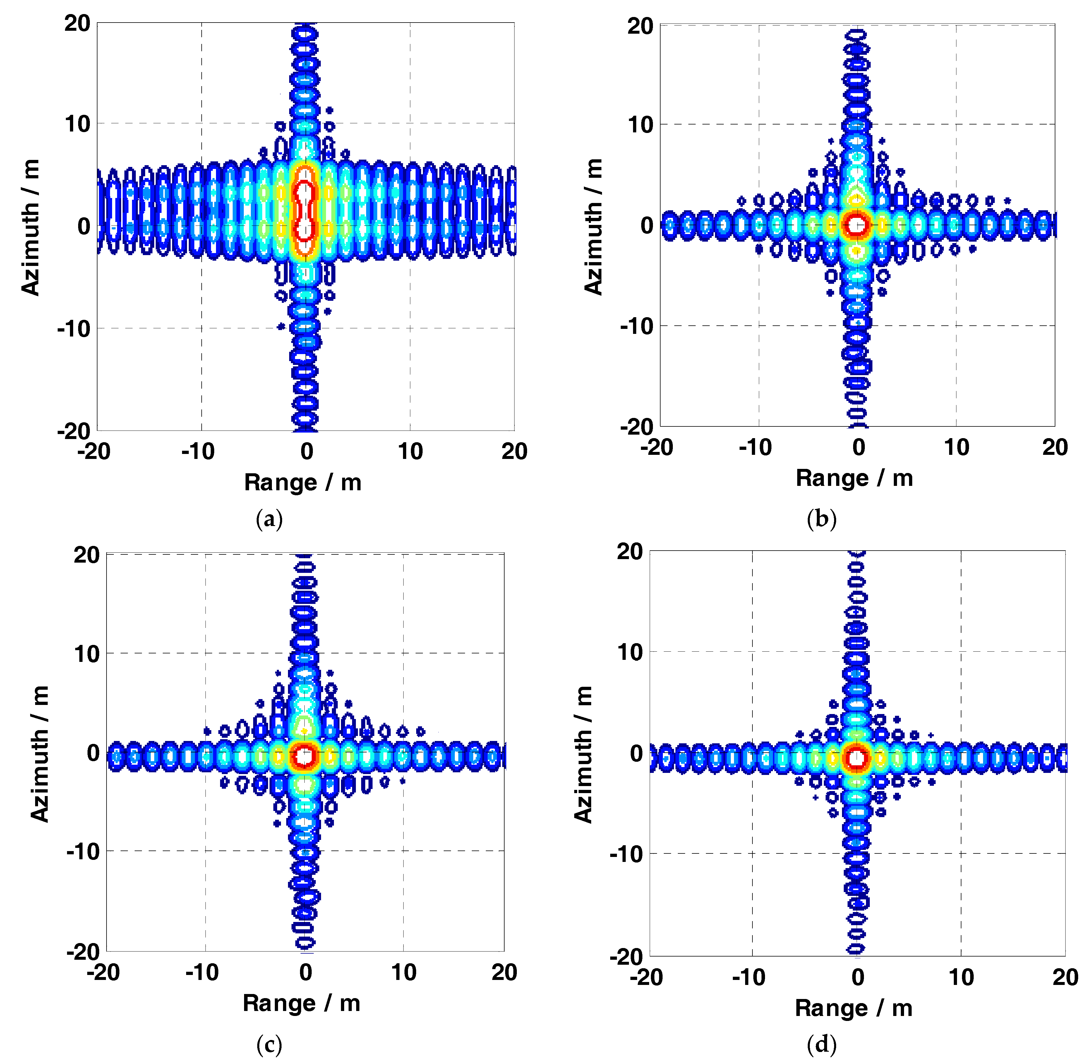
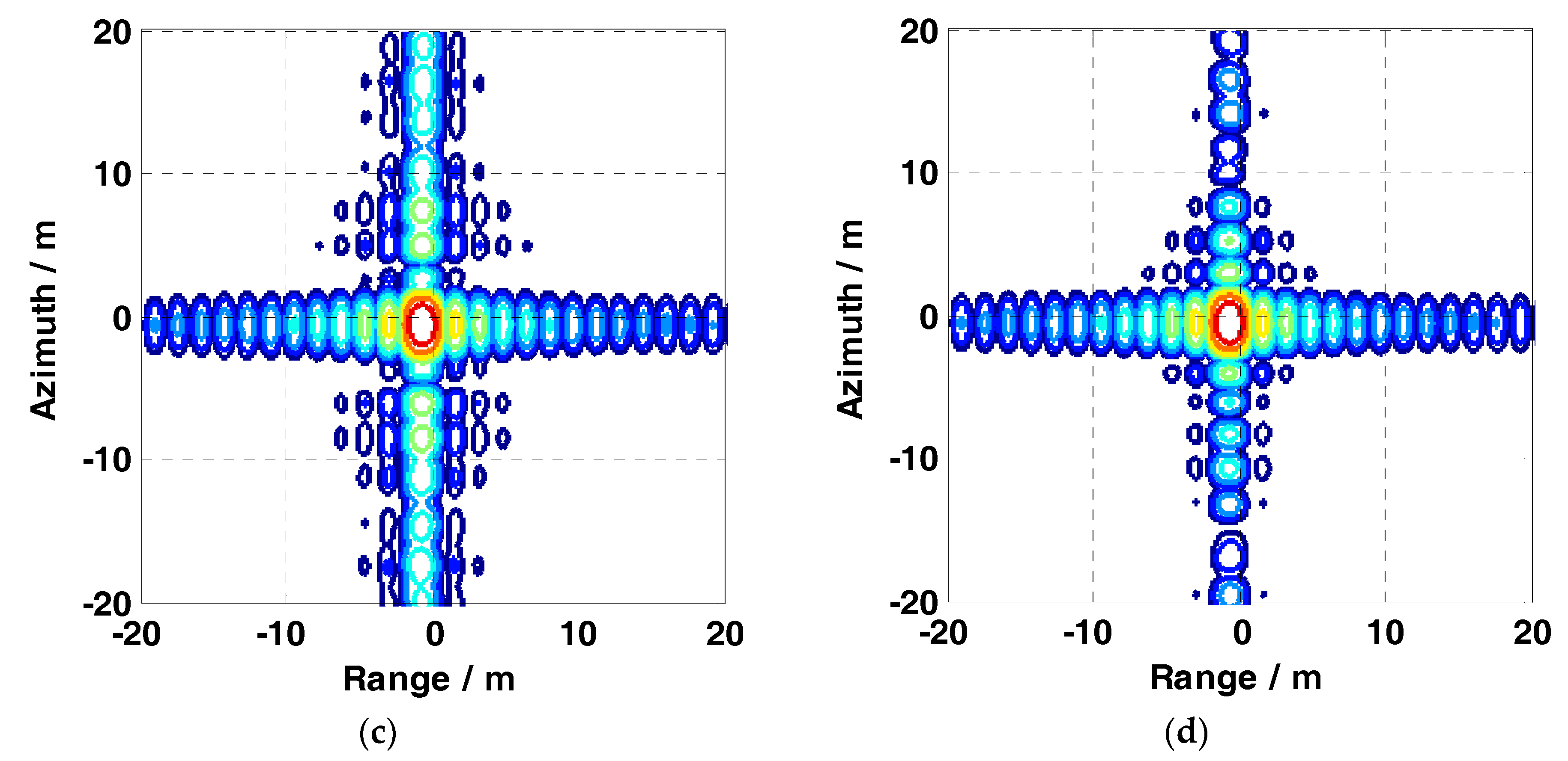
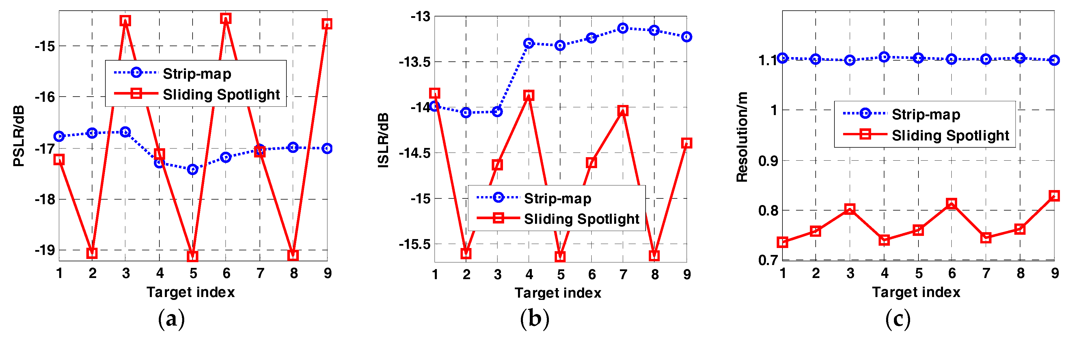
3.1. Simulation Data Processing

3.1.1. Intensive Accelerated Motion Error

In this section, we do a simulation with intensive accelerated motion error to test the validity of the proposed algorithm. A simulation is carried out with parameters listed in

Table 1. Simulation parameters of the intensive accelerated motion error.

Parameters	Values
Center Frequency	9.6 GHz
Bandwidth	100 MHz
Sampling Frequency	120 MHz
Antenna Size (azimuth × range)	2m × 1m
Scene Size (azimuth × range)	1 km × 1 km
Sensor Velocity	150 m/s
Height	9 km
Incidence Angle	76.99°
Pulse Repeat Frequency (PRF)	300 Hz
Pulse Width	30 us
Center Slant Range	40 km
Antenna Azimuth Pattern	Sinc(•)
Motion Error Amplitude	[2 m, 1 m, 2 m]
Motion Error rate	$\left[\frac{\pi }{20},\frac{\pi }{8},\frac{\pi }{20}\right]$
Swath Length	1 km
Echo Acquired Mode	Strip-map

.

Figure 4a shows a 1 km × 1 km scene with dot-matrix targets, and gray dots represent dot-matrix targets. The red squares inserted in Figure 4a represent the assigned target 1–9. We adopt the sinusoidal function to represent the motion error envelope. The initial phases of axes are $\left[\frac{\pi }{6},0,-\frac{\pi }{3}\right]$, respectively. The error of intensive accelerated motion is given in Figure 4b, and we can see that the twitter frequency of the cross direction is much more intensive than the yaw or pitch direction. Figure 4c is its INS output.

After the procession of two-step algorithm, the motion errors along pitch and yaw directions can be neglected as they are mostly suppressed. To make an intuitive comparison, the two-dimensional (2D) simulation results of different algorithms are shown in Figure 5.

MD and PGA algorithms are applied to process the simulated data using the parameters in Table 1. To ensure a fair comparison and clear observation of focus performance, no weighting function or side-lobe control methods are applied. Figure 5 shows the contour maps of target 5, which are processed by conventional SAR imaging, MD, PGA, and BLUE algorithms, respectively. In Figure 5a, it is clear that the result of direct imaging is great degraded along azimuth dimension. It reveals that the residual motion error along cross direction greatly impacts the focusing properties. From Figure 5b–d, it can be concluded that the result processed by the BLUE algorithm performs much better than the ones processed by MD or PGA algorithms, and the focusing quality processed by BLUE algorithm is much improved.

To further evaluate the performance of the estimation, we display the magnitude and phase errors between the non-motion-error echo and data recovered by BLUE algorithm. Figure 6a,b show magnitude and phase errors, respectively. In Figure 6a, the magnitude error is tiny that it can be neglected in the SAR imaging. In Figure 6b, most phase errors are close to 0 rad. The simulation results in Figure 5 show that the BLUE algorithm can recover the echo into a uniform sampling grid.

To evaluate the focusing quality of the proposed algorithm for sliding spotlight SAR, we also carry out an experiment for the sliding spotlight SAR with intensive motion error. The system parameters are the same to Table 1. The angle scanning rate is −0.0013 rad/s. The inserted motion error parameters are also the same as the strip-map SAR, and the results processed by different algorithms are shown in Figure 7.

Figure 7 shows the results processed by different algorithms for sliding spotlight SAR data with intensive accelerated motion error. Comparing Figure 7a–c, we can determine that the autofocusing properties of MD and PGA algorithms are limited in the application of sliding spotlight SAR data with intensive motion error. Figure 7d shows the result processed by the BLUE algorithm, which proves the validity of its autofocusing capability in sliding spotlight SAR data.

3.1.2. Mild Accelerated Motion Error

To further test the validity of the proposed method, a simulation with mild accelerated motion error is executed in this paper. Most of the parameters in this simulation are the same as the Table 1 except for the motion error rate. In this simulation, the motion error rate is substituted by $\left[\frac{\pi }{25},\frac{\pi }{25},\frac{\pi }{25}\right]$.

Figure 8a shows the SAR data simulation with a mild accelerated motion error. Figure 8b is its INS output, and the initial phases of axes are the same as the Figure 4b. The processing results of different algorithms are given in Figure 9.

Figure 9a shows the result of direct SAR imaging algorithm (CS algorithm). Compared with Figure 9a, it is obvious that the focusing quality is still sensitive to the given motion error. Due to the effective velocity and range are azimuth-variance, caused by the given motion error, the serious quadratic phase error (QPE) still exists, although the magnitude and rate are small. A comparison Figure 9b–d demonstrates that the results processed by the BLUE algorithm focuses much better than the ones processed by MD and PGA algorithms.

To show more details of focusing target, we extract the azimuth slices, which are shown in Figure 10, to further compare the focusing properties of the MD, PGA, and BLUE algorithms. The QPE that exists in Figure 10a reveals that the MD algorithm has an infinite focusing ability for this motion error. From Figure 10b, it can be concluded that the PGA algorithm can focus the SAR data well with a mild motion error. However, the residual high order motion error still exists, which results in the asymmetric side-lobe. Figure 10c is the result processed by the BLUE algorithm, and its azimuth slice is close to the ideal point target response. Combined with the results shown in Figure 5d and Figure 7, based on the precise trajectory data measured by GPS or INS, the proposed algorithm can focus the SAR data well with mild or intensive motion error.

In this paper, we also carry out an experiment for the sliding spotlight SAR with mild motion error. The system parameters are same to the simulation of sliding spotlight SAR with intensive motion error. The inserted motion error parameters are also the same as the strip-map SAR with mild accelerated motion error. The results processed by different algorithms are shown in Figure 11.

From Figure 11, we can obtain that MD and PGA algorithm can partly autofocus the sliding spotlight SAR data with mild motion error. Compared with Figure 11b–d, it can be concluded that the result by proposed algorithm has a much better improvement than the MD or PGA algorithm.

3.1.3. Burst-Like Perturbations

To further test the focusing capability of proposed algorithm in the burst-like perturbation, this paper also carries out an experiment in this situation. The system simulation parameters are the same as in Table 1. In the burst-like perturbations simulation, the motion envelope is a Dirac function with a width of 0.25 s, and the error amplitude of the axes is [10 m, 5 m, 10 m], respectively. The error of the axes is given in Figure 12.

Comparing Figure 13a with Figure 13b,c, the improvement of the results processed by the MD or PGA algorithms in autofocusing is largely limited. This demonstrates that the autofocusing property of MD or PGA algorithms is invalid under the burst-like perturbation situation. Figure 13d is the result processed by the BLUE algorithm, which shows a great improvement in focusing compared to the MD or PGA algorithms.

A simulation of sliding spotlight SAR with burst-like perturbations is carried out in this section. The inserted motion error parameters are also the same as the strip-map SAR with burst-like motion error. The results processed by different algorithms are shown in Figure 14.

Compared to Figure 14a–c, Figure 14d focusing performance improves much better than the results processed by MD or PGA algorithms. However, the asymmetric side-lobe along the azimuth dimension still exists.

To further analyze the focusing properties of proposed algorithm, we also count the focusing performances (peak side-lobe ratio (PSLR), integrated side-lobe ratio (ISLR) and resolution) of the targets marked in Figure 4. The performances of the marked targets are given in Figure 15, Figure 16 and Figure 17. They represent the focusing performances for strip and sliding spotlight SAR data with intensive, mild, and burst-like motion errors, respectively.

Comparing Figure 15a–c, it is clear that the focusing performances are stable and close to the nominal values, which prove the validity of the BLUE algorithm in the MOCO for strip-map and sliding spotlight SAR data with intensive motion error. Figure 16 shows the focusing performances for SAR data with mild motion error. The distributions of performances are smooth. Combined with Figure 9d and Figure 11d, the results and performance distribution reveals the validity of the BLUE algorithm.

From Figure 17, the focusing performance distributions of the sliding spotlight SAR are more unsteady than that of the strip-map SAR. For burst-like perturbations, the proposed algorithm can better focus the strip-map SAR data than the sliding spotlight SAR data. Indeed, it has much better improvement than MD or PGA algorithms.

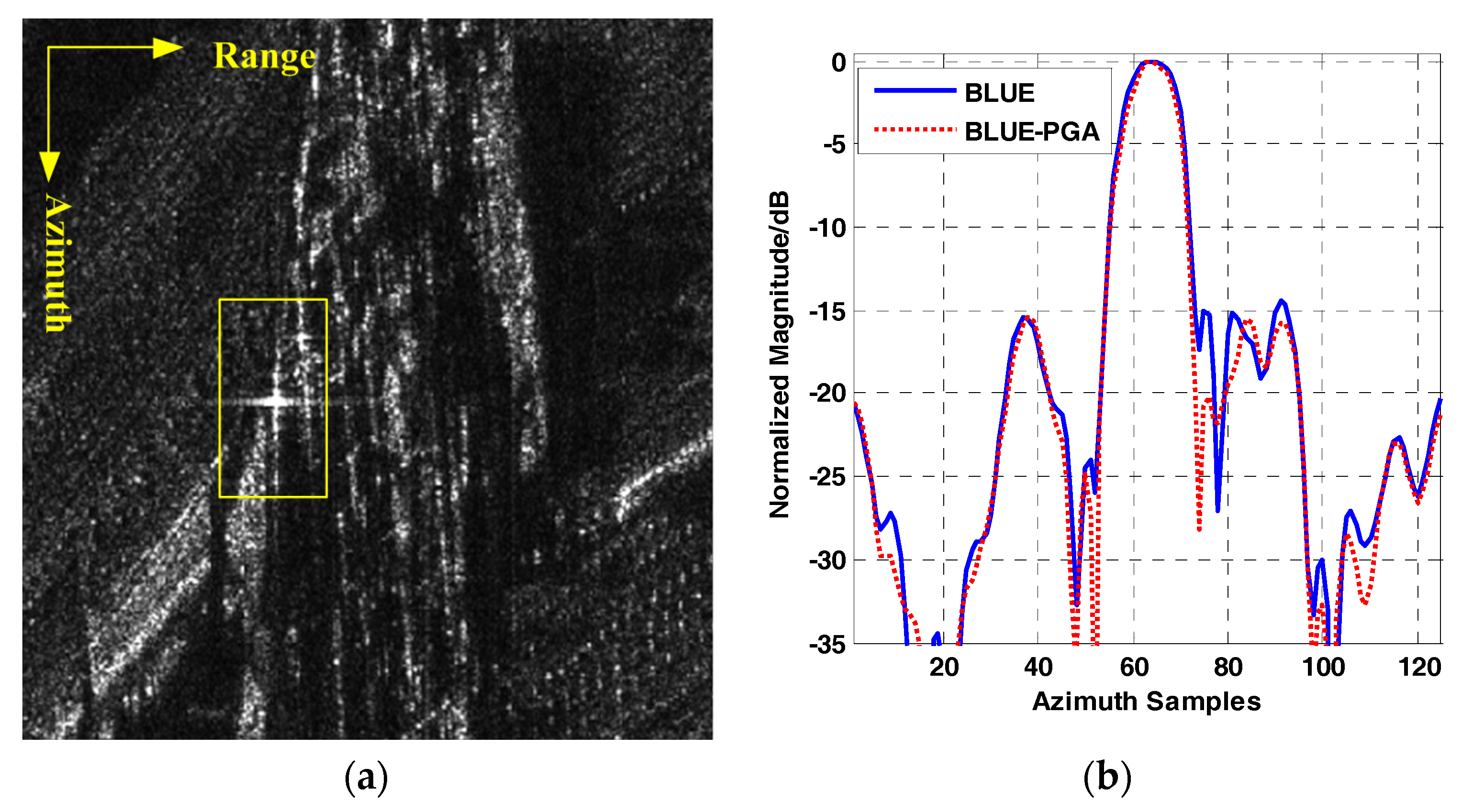
3.2. Real Data Processing

We consider a real data case to further validate the proposed algorithm. The data is obtained from a 5 km × 26 km scene, with a bandwidth of 80 MHz centering at 9.6 GHz. Firstly, we adopt the two-step algorithm to correct the motion error along the pitch and yaw. Figure 10b represents the result processed by CS algorithm. Figure 18c–e show close views of the yellow rectangular area processed by the MD, PGA, and BLUE algorithms, respectively. Scene details and grains are much clear in the result processed by BLUE algorithm (Figure 18e) than the cases processed by MD (Figure 18c) or PGA algorithms (Figure 18d). Due to the space limitation, we only show the area in the yellow rectangle, but the outcomes hold for the complete scene.

Figure 18f,g shows the azimuth slice of corner reflector marked with a yellow rectangle in Figure 18b–e. The corner reflector amplitude in Figure 18f,g are represented by linear and log, respectively. The blue solid, green dashed, dark and red lines are the processing results of the direct imaging (after processing of two-step algorithm), MD, PGA, and BLUE algorithms, respectively. Figure 18f,g, reveals that the power of the result processed by the BLUE algorithm is more focused in the main-lobe than the results processed by the MD or PGA algorithms. In Figure 18g, it can be determined that the azimuth response of result processed by BLUE algorithm is close to the ideal azimuth response. The side-lobe shape and magnitude reveals the existence of the residual high-order error.

Figure 18h–k shows the homogeneous scene results processed by different algorithms. From Figure 18k, processed by the BLUE algorithm, it can be concluded that the grains are much clear than the results processed than MD or PGA algorithm.

To further evaluate the performance of the proposed algorithm, we calculate the entropy of Figure 18b–e and Figure 18h–k. The entropy value is given in

Table 2. Entropy of images processed by different algorithms.

Scene Type	Images Processed by Different Algorithm	Entropy Values
Strong backscatters	Origin	6.5928
	MD	6.5262
	PGA	6.4922
	BLUE	6.4694
Homogeneous backscatters	Origin	7.0883
	MD	7.0739
	PGA	7.0080
	BLUE	6.9579

.

In strong backscatters or homogeneous region, the entropy of image processed by BLUE algorithm is the minimum in Table 2. Combining with the azimuth responses shown in Figure 10f,g, it can be concluded that the entropy of images prove the validity of the proposed algorithm.

To improve the quality of the image in focus, the autofocusing is applied after the processing of the BLUE algorithm. The results are given in Figure 19. Figure 19a shows the result processed by the combination of the BLUE and PGA algorithms (BLUE-PGA), and the entropy of Figure 19a is 6.4661. The input of the PGA is the imaging result of Figure 18e. Figure 19b shows the azimuth slices of the BLUE and BLUE-PGA algorithms. The comparison reveals that the BLUE algorithm can ensure the focusing quality on the premise of acquiring the precise trajectory data.

4. Discussion

4.1. Impact of the Two-Step Residual Error

In Section 2, we assume that the two-step algorithm can correct the motion error along X and Z axes. However, there exists the residual motion error after the processing of two-step algorithm. The residual motion error results in the effective sampling position deviating from the position $y_a\left(\eta \right)$. Generally speaking, the residual error often appears by the envelope of low-frequency or high-frequency. In this section, we take two types of residual error, linear error (low-frequency), and high-order sine error (high-frequency), into consideration to discuss the impact of the two-step residual error. The amplitudes of linear and high-order sine error are 1 m and 0.03 m, respectively. The rate of high-order sine error is 0.1 Hz. The motion error of Y axis is same as the one in Section 3.1.2. The processing results are given in Figure 20 and Figure 21.

Figure 20 and Figure 21 show the results proposed by different algorithms for strip-map SAR data with linear and high-order sine residual motion error, respectively. From Figure 20d and Figure 21d, it reveals that the residual error of the two-step algorithm degrades the focusing quality of the proposed algorithm. However, the focusing performances of the results processed by the BLUE algorithm are still much better than the ones processed by the MD or PGA algorithms.

4.2. Impact of Positioning Error

From Section 2 and Section 3, we obtain that, based on the precise trajectory data, the BLUE algorithm has much better focusing performances in the MOCO than the MD and PGA algorithms. GPS has the capability of high-precision positioning, however, its response time is long for SAR. INS can record the platform position in real-time, which is coincided with the azimuth fast sampling of SAR. Yet its positioning error is accumulated with the working time. In most airborne SAR missions, GPS and INS are mounted in the platform simultaneously to obtain the high-precision positioning data by merging the data recorded by GPS and INS [14]. However, limited by the space and power, the unmanned airborne SAR either chooses GPS or INS as its positioning device. This means that it is not easy to obtain precise trajectory data for unmanned airborne SAR.

Caused by motion error, radar samples the echo deviating from the ideal space position, which essentially results in non-uniform sampling. The conventional frequency domain imaging algorithms use Fast Fourier Transform (FFT) to achieve fast SAR imaging. However, FFT is just applied in the uniform sampling data. This is the main defocusing reason for airborne SAR with motion error. From Section 2, we know that the BLUE algorithm recovers the SAR data with motion error to a uniform sampling grid. In this section, we will discuss the focusing influence of the proposed algorithm without precise trajectory data.

The positioning error of a single ordinary dual-frequency GPS device is around 0.2 m [15]. Simulation parameters of the GPS positioning error is given in

Table 3. Simulation parameters of positioning error.

Parameters	Value
GPS error distribution	random noise
GPS error magnitude	0.2 m
INS error distribution	quadratic function

. We assume that the distributions of GPS and INS positioning errors obey the random noise and quadratic function, respectively.

Figure 22 shows positioning device error and its imaging result processed by the BLUE algorithm. From Figure 22b,d, we can obtain that the positioning error caused by the device results in the defocusing of SAR data. This reveals that the BLUE algorithm is limited by the precision of the positioning device.

4.3. Comparison of the Computational Cost

From Equation (13), we can obtain the number of useful PSD auto-coefficients in the estimation of the proposed algorithm:

$$N_{\mathrm{useful}}=2\lceil \frac{L_a}{V_r}·\mathrm{PRF}\rceil$$

(17)

For strip-map SAR, the variables in Equation (17) have the following coupling relationship:

$$\begin{array}{l}{L}_a\approx 2{\rho }_a\\ {\rho }_a\approx \frac{V_r}{B_a}\\ \mathrm{PRF}=\alpha B_a\end{array}$$

(18)

where ${\rho }_a$, $B_a$ and $\alpha$ represent the azimuth resolution, azimuth bandwidth, and azimuth oversampling rate, respectively. Hence, Equation (17) can be approximately expressed as:

$$N_{\mathrm{useful}}=2\lceil 2\alpha \rceil$$

(19)

assuming that the size of the echo is $N_r$ × $N_a$ (range: x azimuth), and the computational costs of MD, PGA, and BLUE algorithms are given in

Table 4. Computational costs of different algorithms.

Algorithms	Computational Costs
MD	$10N_r{N}_a{\log }_2\left(N_a\right)+\left(N_{\mathrm{sub}}-1\right)N_r{N}_a$
PGA	$10N_r{N}_a{\log }_2\left(N_a\right)+2N_r{N}_a$
BLUE	$2N_{\mathrm{useful}}^2{N}_r{N}_a$

.

$N_{\mathrm{sub}}$ represents the number of subapertures in the application of the MD algorithm. For a SAR system, the typical value of $\alpha$ is less than 2. We carry out a computational cost comparison of different algorithms. The number of azimuth samples $N_a$ varies from 128 to 8192. The other parameter values are given in Figure 23.

From Figure 23 and Table 4, it is obvious that the computational cost of BLUE is much lower than the MD or PGA algorithms.

5. Conclusions

The proposed algorithm has been applied to the MOCO of airborne SAR data and significantly improves the images captured under varying acceleration and velocity compared with the results achieved by MD and PGA algorithms.

Based on the precise trajectory, the proposed algorithm also provides superior autofocus capability for a uniformly distributed backscatter scene compared with the MD and PGA algorithms. In this paper, we also discuss the focusing property of proposed algorithm without the precise trajectory. The simulation results reveal that the focusing performances of the proposed algorithm are greatly limited by the precision of the positioning devices. Additionally, it would limit the proposed algorithm applied to the unmanned SAR data. Although the BLUE algorithm accuracy depends on positioning device precision, i.e., GPS or INS, precise GPS or INS systems are relatively cheap and are commonly employed for SAR data collection. Thus, the proposed algorithm may have great potential in the imaging application of SAR data with precise trajectory data.

References

1. Prats, P.; Scheiber, R.; Mittermayer, J.; Meta, A.; Moreira, A. Processing of Sliding Spotlight and TOPS SAR Data Using Baseband Azimuth Scaling. IEEE Trans. Geosci. Remote Sens. 2010, 48, 770–780. [Google Scholar] [CrossRef] [Green Version]
2. Xu, Z.; Chen, K.S. On Signal Modeling of Moon-Based Synthetic Aperture Radar (SAR) Imaging of Earth. Remote Sens. 2018, 10, 486. [Google Scholar] [CrossRef]
3. Zhang, S.; Xu, Q.; Zheng, Q.; Li, X. Mechanisms of SAR Imaging of Shallow Water Topography of the Subei Bank. Remote Sens. 2017, 9, 1203. [Google Scholar] [CrossRef]
4. Fornaro, G. Trajectory Deviations in Airborne SAR: Analysis and Compensation. IEEE Trans. Aerosp. Electron. Syst. 1999, 35, 997–1009. [Google Scholar] [CrossRef]
5. Shi, J.; Ma, L.; Zhang, X. Streaming BP for Non-Linear Motion Compensation SAR Imaging Based on GPU. IEEE J. Sel. Top Appl. Earth Observ. Remote Sens. 2013, 6, 2035–2050. [Google Scholar]
6. Moreira, J.R. A New Method of Aircraft Motion Error Extraction from Radar Raw Data for Real Time Motion. IEEE Trans. Geosci. Remote Sens. 1990, 28, 620–626. [Google Scholar] [CrossRef]
7. Zhang, L.; Hu, M.; Wang, G.; Wang, H. Range-Dependent Map-Drift algorithm for Focusing UAV SAR Imagery. IEEE Geosci. Remote. Sens. Lett. 2016, 13, 1158–1162. [Google Scholar] [CrossRef]
8. Wahl, D.E.; Jakowatz, C.V.; Thompson, P.A.; Ghiglia, D.C. New Approach to Strip-map SAR Autofocus. In Proceedings of the IEEE 6th Digital Signal Processing Workshop, Yosemite National Park, CA, USA, 2–5 October 1994; pp. 53–56. [Google Scholar]
9. Eichel, P.H.; Ghiglia, D.C.; Jakowatz, C.V. Speckle processing method for synthetic-aperture-radar phase correction. Optics Lett. 1989, 14, 1–3. [Google Scholar] [CrossRef]
10. Xiong, T.; Xing, M.; Wang, Y.; Wang, S.; Sheng, J.; Guo, L. Minimum-Entropy-Based Autofocus Algorithm for SAR Data Using Chebyshev Approximation and Method of Series Reversion and Its Implementation in a Data Processor. IEEE Trans. Geosci. Remote Sens. 2014, 52, 1719–1728. [Google Scholar] [CrossRef]
11. Kay, S.M. Fundamentals of Statistical Signal Processing: Estimation Theory; Prentice Hall: Englewood Cliffs, NJ, USA, 1993. [Google Scholar]
12. Meta, A.; Prats, P.; Steinbrecher, U.; Mittermayer, J.; Scheiber, R. TerraSAR-X TOPSAR and ScanSAR comparison. In Proceedings of the 7th European Conference on Synthetic Aperture Radar, Friedrichshafen, Germany, 2–5 June 2008. [Google Scholar]
13. Meta, A.; Mittermayer, J.; Prats, P.; Scheiber, R.; Steinbrecher, U. TOPS Imaging with TerraSAR-X: Mode Design and Performance Analysis. IEEE Trans. Geosci. Remote Sens. 2010, 48, 759–769. [Google Scholar] [CrossRef] [Green Version]
14. Xing, M.; Jiang, X.; Wu, R.; Zhou, F.; Bao, Z. Motion Compensation for UAV SAR Based on Raw Data. IEEE Trans. Geosci. Remote Sens. 2009, 47, 2870–2883. [Google Scholar] [CrossRef]
15. Kou, K.H.; Zhang, Y.A.; Liu, A.L. Vision-aided INS fast localization error modification method for cruise missiles. Syst. Eng. Electron. 2013, 35, 397–401. [Google Scholar]
Figure 1. Geometry of the airborne SAR with motion error.
Remotesensing 10 01124 g001
Figure 2. Sample geometry after the initial motion compensation.
Remotesensing 10 01124 g002
Figure 3. Blocks of the BLUE processing procedures.
Remotesensing 10 01124 g003
Figure 4. (a) Airborne SAR geometry with motion error and scene with target dots. (b) Error of intensive accelerated motion. (c) INS output.
Remotesensing 10 01124 g004
Figure 5. Target 5’s contours processed by (a) the conventional SAR imaging algorithm (CS algorithm), (b) MD algorithm, (c) PGA algorithm, and (d) BLUE algorithm, for strip-map SAR data with intensive accelerated motion error.
Remotesensing 10 01124 g005
Figure 6. Magnitude and phase errors between the non-motion-error echo and data recovered by BLUE algorithm. (a,b) are magnitude and phase errors, respectively.
Remotesensing 10 01124 g006
Figure 7. Target 5’s contours processed by (a) the conventional SAR imaging algorithm (CS algorithm), (b) MD algorithm, (c) PGA algorithm, and (d) BLUE algorithm, for sliding spotlight SAR data with intensive accelerated motion error.
Remotesensing 10 01124 g007aRemotesensing 10 01124 g007b
Figure 8. (a) Error of mild accelerated motion. (b) INS output.
Remotesensing 10 01124 g008
Figure 9. Target 5’s contours processed by (a) the conventional SAR imaging algorithm (CS algorithm), (b) MD algorithm, (c) PGA algorithm, and (d) BLUE algorithm, for SAR data with mild accelerated motion error.
Remotesensing 10 01124 g009
Figure 10. Target 5’s azimuth slices processed by (a) MD algorithm, (b) PGA algorithm, and (c) BLUE algorithm, for strip-map SAR with mild accelerated motion error.
Remotesensing 10 01124 g010
Figure 11. Target 5’s contours processed by (a) the conventional SAR imaging algorithm (CS algorithm), (b) MD algorithm, (c) PGA algorithm, and (d) BLUE algorithm, for sliding spotlight SAR data with mild accelerated motion error.
Remotesensing 10 01124 g011
Figure 12. Burst-like perturbation error of the axes.
Remotesensing 10 01124 g012
Figure 13. Target 5’s contours processed by (a) the conventional SAR imaging algorithm (CS algorithm), (b) MD algorithm, (c) PGA algorithm, and (d) BLUE algorithm, for strip-map SAR data with burst-like perturbation errors.
Remotesensing 10 01124 g013aRemotesensing 10 01124 g013b
Figure 14. Target 5’s contours processed by (a) the conventional SAR imaging algorithm (CS algorithm), (b) MD algorithm, (c) PGA algorithm, and (d) BLUE algorithm, for sliding spotlight SAR data with burst-like perturbations.
Remotesensing 10 01124 g014aRemotesensing 10 01124 g014b
Figure 15. Distribution of focusing performances for SAR data with intensive motion error. (ac) are the distributions of PSLR, ISLR, and resolution, respectively. The blue dashed line and red one are the results of strip-map and sliding spotlight, respectively.
Remotesensing 10 01124 g015
Figure 16. Distribution of focusing performances for SAR data with mild motion error. (ac) are the distributions of PSLR, ISLR, and resolution, respectively. The blue dashed line and red one are the results of strip-map and sliding spotlight, respectively.
Remotesensing 10 01124 g016
Figure 17. Distribution of focusing performances for SAR data with burst-like perturbations. (ac) are the distributions of PSLR, ISLR, and resolution, respectively. The blue dashed line and red one are the results of strip-map and sliding spotlight, respectively.
Remotesensing 10 01124 g017
Figure 18. Actual SAR image and analysis. (a) Full scene image, and close views of the yellow rectangle processed using (b) CS, (c) MD, (d) PGA, and (d) BLUE algorithms. (f,g), represented by linear and log, are azimuth slices of the corner reflector marked with a yellow rectangle in (be). (hk) are close views of the yellow ellipse processed by the CS, MD, PGA, and BLUE algorithm, respectively. The azimuth direction is vertical.
Remotesensing 10 01124 g018aRemotesensing 10 01124 g018b
Figure 19. (a) Result processed by the combination of the BLUE and PGA (BLUE-PGA) algorithms. (b) Azimuth slices of the BLUE and BLUE-PGA algorithms.
Remotesensing 10 01124 g019
Figure 20. Target 5’s contours processed by (a) the conventional SAR imaging algorithm (CS algorithm), (b) the MD algorithm, (c) the PGA algorithm, and (d) the BLUE algorithm, for strip SAR data with linear residual motion error.
Remotesensing 10 01124 g020
Figure 21. Target 5’s contours processed by (a) the conventional SAR imaging algorithm (CS algorithm), (b) the MD algorithm, (c) the PGA algorithm, and (d) the BLUE algorithm, for strip SAR data with high-order sine residual motion error.
Remotesensing 10 01124 g021
Figure 22. Simulation results with positioning error. (a) GPS positioning error. (b) Target 5’s contour result with GPS positioning error. (c) INS positioning error. (d) Target 5’s contour result with INS positioning error.
Remotesensing 10 01124 g022aRemotesensing 10 01124 g022b
Figure 23. Computational cost comparison of different algorithms. The blue line, dark dashed one, and red dot-dashed one are the computational costs of MD, PGA, and BLUE algorithms, respectively.
Remotesensing 10 01124 g023