Combining Linear Pixel Unmixing and STARFM for Spatiotemporal Fusion of Gaofen-1 Wide Field of View Imagery and MODIS Imagery


Abstract
1. Introduction
2. Study Area and Datasets
2.1. Study Area
2.2. Datasets
2.2.1. GF-1 WFV Data
2.2.2. MODIS Data
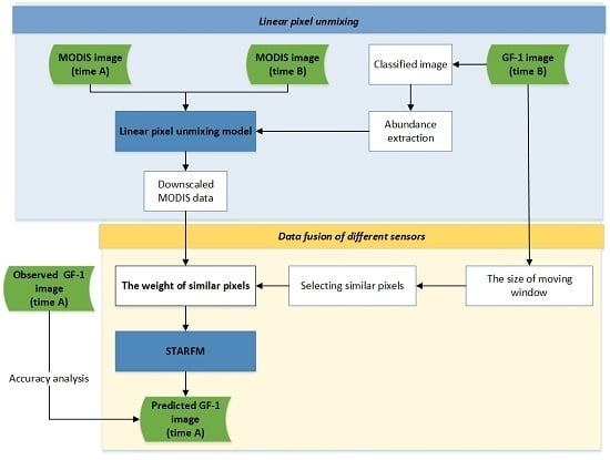
3. Methodology
3.1. MODIS Linear Spectral Mixture Analysis
Endmember Selection and Fraction Calculation
3.2. The Theoretical Basis of the STARFM
3.3. Data Quality Evaluation Method of Spatiotemporal Fusion
4. Results
4.1. Spectral Mixture Analysis of MODIS Data
4.2. The Fusion of High Spatial and Temporal Resolution Imagery
4.2.1. Qualitative Analysis of the Fusion Imagery
4.2.2. Quantitative Analysis of the Fusion Imagery
4.3. The Comparison of Estimation Accuracy of Reflectance in Homogeneous/Heterogeneous Areas
4.4. NDVI Estimation and Comparative Analysis
5. Discussion
- (1)
- The differences in multi-source remote sensing data. Due to different measurement principles and observation environments, different sensors have different spectral settings and spectral response functions. In addition, errors such as radiation calibration, atmospheric correction, and geometric correction are unavoidable in data processing. These are nonlinear factors that cause systematic errors within sensor data.
- (2)
- The change in land cover types. The date of the prediction imagery and the reference imagery of the STARFM algorithm should be within a season. If the time interval is too long, land cover changes become more likely, and the corresponding relationship between the band reflectance data before and after fusion is not maintained well, resulting in a decrease in the precision of prediction results. Therefore, the selection of reference images should be taken into consideration in fusion.
- (3)
- The variability of reflectance of pixels. The linear spectral mixture model is based on the assumption that the same land cover types have the same spectral features, and that there is a linear summation of the spectra. In fact, the spectral reflectance of each land cover type is combined in nonlinear forms and has variability. In addition, due to randomness and variability, natural, random residuals are unavoidable. All these factors may affect the accuracy of the model and the results of spectral mixture analysis.
6. Conclusions
Author Contributions
Funding
Acknowledgments
Conflicts of Interest
References
- Coops, N.C.; Johnson, M.; Wulder, M.A.; White, J.C. Assessment of QuickBird high spatial resolution imagery to detect red attack damage due to mountain pine beetle infestation. Remote Sens. Environ. 2006, 103, 67–80. [Google Scholar] [CrossRef]
- Tian, F.; Wang, Y.J.; Fensholt, R.; Wang, K.; Zhang, L.; Huang, Y. Mapping and Evaluation of NDVI Trends from Synthetic Time Series Obtained by Blending Landsat and MODIS Data around a Coalfield on the Loess Plateau. Remote Sens. 2013, 5, 4255–4279. [Google Scholar] [CrossRef]
- Jarihani, A.A.; McVicar, T.R.; Van Niel, T.G.; Emelyanova, I.V.; Callow, J.N.; Johansen, K. Blending Landsat and MODIS Data to Generate Multispectral Indices: A Comparison of “Index-then-Blend” and “Blend-then-Index” Approaches. Remote Sens. 2014, 6, 9213–9238. [Google Scholar] [CrossRef]
- Tewes, A.; Thonfeld, F.; Schmidt, M.; Oomen, R.J.; Zhu, X.L.; Dubovyk, O.; Menz, G.; Schellberg, J. Using RapidEye and MODIS Data Fusion to Monitor Vegetation Dynamics in Semi-Arid Rangelands in South Africa. Remote Sens. 2015, 7, 6510–6534. [Google Scholar] [CrossRef]
- Rao, Y.H.; Zhu, X.L.; Chen, J.; Wang, J.M. An Improved Method for Producing High Spatial-Resolution NDVI Time Series Datasets with Multi-Temporal MODIS NDVI Data and Landsat TM/ETM plus Images. Remote Sens. 2015, 7, 7865–7891. [Google Scholar] [CrossRef]
- Schmidt, M.; Udelhoven, T.; Gill, T.; Roder, A. Long term data fusion for a dense time series analysis with MODIS and Landsat imagery in an Australian Savanna. J. Appl. Remote Sens. 2012, 6, 063512. [Google Scholar]
- Zhang, W.; Li, A.N.; Jin, H.A.; Bian, J.H.; Zhang, Z.J.; Lei, G.B.; Qin, Z.H.; Huang, C.Q. An Enhanced Spatial and Temporal Data Fusion Model for Fusing Landsat and MODIS Surface Reflectance to Generate High Temporal Landsat-Like Data. Remote Sens. 2013, 5, 5346–5368. [Google Scholar] [CrossRef]
- Bai, Y.; Wong, M.S.; Shi, W.Z.; Wu, L.X.; Qin, K. Advancing of Land Surface Temperature Retrieval Using Extreme Learning Machine and Spatio-Temporal Adaptive Data Fusion Algorithm. Remote Sens. 2015, 7, 4424–4441. [Google Scholar] [CrossRef]
- Singh, D. Generation and evaluation of gross primary productivity using Landsat data through blending with MODIS data. Int. J. Appl. Earth Obs. Geoinf. 2011, 13, 59–69. [Google Scholar] [CrossRef]
- Weng, Q.H.; Fu, P.; Gao, F. Generating daily land surface temperature at Landsat resolution by fusing Landsat and MODIS data. Remote Sens. Environ. 2014, 145, 55–67. [Google Scholar] [CrossRef]
- Chen, B.; Ge, Q.; Fu, D.; Yu, G.; Sun, X.; Wang, S.; Wang, H. A data-model fusion approach for upscaling gross ecosystem productivity to the landscape scale based on remote sensing and flux footprint modelling. Biogeosciences 2010, 7, 2943–2958. [Google Scholar] [CrossRef]
- Liu, K.; Su, H.B.; Li, X.K.; Wang, W.M.; Yang, L.J.; Liang, H. Quantifying Spatial-Temporal Pattern of Urban Heat Island in Beijing: An Improved Assessment Using Land Surface Temperature (LST) Time Series Observations From LANDSAT, MODIS, and Chinese New Satellite GaoFen-1. IEEE J. Sel. Top. Appl. Earth Obs. Remote Sens. 2016, 9, 2028–2042. [Google Scholar] [CrossRef]
- Chao, Y.F.; Zhang, H.T.; Dan, G.; Hao, W. Wetland mapping and wetland temporal dynamic analysis in the Nanjishan wetland using Gaofen One data. Ann. GIS 2016, 22, 259–271. [Google Scholar]
- Wu, M.Q.; Huang, W.J.; Niu, Z.; Wang, C.Y. Combining HJ CCD, GF-1 WFV and MODIS Data to Generate Daily High Spatial Resolution Synthetic Data for Environmental Process Monitoring. Int. J. Environ. Res. Public Health 2015, 12, 9920–9937. [Google Scholar] [CrossRef] [PubMed]
- Fu, B.L.; Wang, Y.Q.; Campbell, A.; Li, Y.; Zhang, B.; Yin, S.B.; Xing, Z.F.; Jin, X.M. Comparison of object-based and pixel-based Random Forest algorithm for wetland vegetation mapping using high spatial resolution GF-1 and SAR data. Ecol. Indic. 2017, 73, 105–117. [Google Scholar] [CrossRef]
- Li, J.; Chen, X.L.; Tian, L.Q.; Huang, J.; Feng, L. Improved capabilities of the Chinese high-resolution remote sensing satellite GF-1 for monitoring suspended particulate matter (SPM) in inland waters: Radiometric and spatial considerations. ISPRS J. Photogramm. Remote Sens. 2015, 106, 145–156. [Google Scholar] [CrossRef]
- Song, Q.; Hu, Q.; Zhou, Q.B.; Hovis, C.; Xiang, M.T.; Tang, H.J.; Wu, W.B. In-Season Crop Mapping with GF-1/WFV Data by Combining Object-Based Image Analysis and Random Forest. Remote Sens. 2017, 9, 1184. [Google Scholar] [CrossRef]
- Marchane, A.; Jarlan, L.; Hanich, L.; Boudhar, A.; Gascoin, S.; Tavernier, A.; Filali, N.; Le Page, M.; Hagolle, O.; Berjamy, B. Assessment of daily MODIS snow cover products to monitor snow cover dynamics over the Moroccan Atlas mountain range. Remote Sens. Environ. 2015, 160, 72–86. [Google Scholar] [CrossRef]
- Chen, Y.L.; Song, X.D.; Wang, S.S.; Huang, J.F.; Mansaray, L.R. Impacts of spatial heterogeneity on crop area mapping in Canada using MODIS data. ISPRS J. Photogramm. Remote Sens. 2016, 119, 451–461. [Google Scholar] [CrossRef]
- Portillo-Quintero, C.A.; Sanchez, A.M.; Valbuena, C.A.; Gonzalez, Y.Y.; Larreal, J.T. Forest cover and deforestation patterns in the Northern Andes (Lake Maracaibo Basin): A synoptic assessment using MODIS and Landsat imagery. Appl. Geogr. 2012, 35, 152–163. [Google Scholar] [CrossRef]
- Wu, M.Q.; Wu, C.Y.; Huang, W.J.; Niu, Z.; Wang, C.Y.; Li, W.; Hao, P.Y. An improved high spatial and temporal data fusion approach for combining Landsat and MODIS data to generate daily synthetic Landsat imagery. Inf. Fusion 2016, 31, 14–25. [Google Scholar] [CrossRef]
- Zhukov, B.; Oertel, D.; Lanzl, F.; Reinhackel, G. Unmixing-based multisensor multiresolution image fusion. IEEE Trans. Geosci. Remote Sens. 1999, 37, 1212–1226. [Google Scholar] [CrossRef]
- Maselli, F. Definition of spatially variable spectral endmembers by locally calibrated multivariate regression analyses. Remote Sens. Environ. 2001, 75, 29–38. [Google Scholar] [CrossRef]
- Busetto, L.; Meroni, M.; Colombo, R. Combining medium and coarse spatial resolution satellite data to improve the estimation of sub-pixel NDVI time series. Remote Sens. Environ. 2008, 112, 118–131. [Google Scholar] [CrossRef]
- Cherchali, S.; Amram, O.; Flouzat, G. Retrieval of temporal profiles of reflectances from simulated and real NOAA-AVHRR data over heterogeneous landscapes. Int. J. Remote Sens. 2000, 21, 753–775. [Google Scholar] [CrossRef]
- Gao, F.; Masek, J.; Schwaller, M.; Hall, F. On the blending of the Landsat and MODIS surface reflectance: Predicting daily Landsat surface reflectance. IEEE Trans. Geosci. Remote Sens. 2006, 44, 2207–2218. [Google Scholar]
- Walker, J.J.; de Beurs, K.M.; Wynne, R.H.; Gao, F. Evaluation of Landsat and MODIS data fusion products for analysis of dryland forest phenology. Remote Sens. Environ. 2012, 117, 381–393. [Google Scholar] [CrossRef]
- Swain, R.; Sahoo, B. Mapping of heavy metal pollution in river water at daily time-scale using spatio-temporal fusion of MODIS-aqua and Landsat satellite imageries. J. Environ. Manag. 2017, 192, 1–14. [Google Scholar] [CrossRef] [PubMed]
- Walker, J.J.; de Beurs, K.M.; Wynne, R.H. Dryland vegetation phenology across an elevation gradient in Arizona, USA, investigated with fused MODIS and Landsat data. Remote Sens. Environ. 2014, 144, 85–97. [Google Scholar] [CrossRef]
- Olsoy, P.J.; Mitchell, J.; Glenn, N.F.; Flores, A.N. Assessing a Multi-Platform Data Fusion Technique in Capturing Spatiotemporal Dynamics of Heterogeneous Dryland Ecosystems in Topographically Complex Terrain. Remote Sens. 2017, 9, 981. [Google Scholar] [CrossRef]
- Hilker, T.; Wulder, M.A.; Coops, N.C.; Seitz, N.; White, J.C.; Gao, F.; Masek, J.G.; Stenhouse, G. Generation of dense time series synthetic Landsat data through data blending with MODIS using a spatial and temporal adaptive reflectance fusion model. Remote Sens. Environ. 2009, 113, 1988–1999. [Google Scholar] [CrossRef]
- Hilker, T.; Wulder, M.A.; Coops, N.C.; Linke, J.; McDermid, G.; Masek, J.G.; Gao, F.; White, J.C. A new data fusion model for high spatial- and temporal-resolution mapping of forest disturbance based on Landsat and MODIS. Remote Sens. Environ. 2009, 113, 1613–1627. [Google Scholar] [CrossRef]
- Roy, D.P.; Ju, J.; Lewis, P.; Schaaf, C.; Gao, F.; Hansen, M.; Lindquist, E. Multi-temporal MODIS-Landsat data fusion for relative radiometric normalization, gap filling, and prediction of Landsat data. Remote Sens. Environ. 2008, 112, 3112–3130. [Google Scholar] [CrossRef]
- Zhu, X.L.; Chen, J.; Gao, F.; Chen, X.H.; Masek, J.G. An enhanced spatial and temporal adaptive reflectance fusion model for complex heterogeneous regions. Remote Sens. Environ. 2010, 114, 2610–2623. [Google Scholar] [CrossRef]
- Yang, J.C.; Wright, J.; Huang, T.; Ma, Y. Image super-resolution via sparse representation. IEEE Trans. Image Process. 2010, 19, 2861–2873. [Google Scholar] [CrossRef] [PubMed]
- Zeyde, R.; Elad, M.; Protter, M. On Single Image Scale-Up Using Sparse Representations. In Proceedings of the 7th International Conference on Curves and Surfaces, Avignon, France, 24–30 June 2012; pp. 711–730. [Google Scholar]
- Song, H.H.; Huang, B. Spatiotemporal Satellite Image Fusion through One-Pair Image Learning. IEEE Trans. Geosci. Remote Sens. 2013, 51, 1883–1896. [Google Scholar] [CrossRef]
- Vermote, E.F.; Tanre, D.; Deuze, J.L.; Herman, M.; Morcrette, J.J. Second Simulation of the Satellite Signal in the Solar Spectrum, 6S: An overview. IEEE Trans. Geosci. Remote Sens. 1997, 35, 675–686. [Google Scholar] [CrossRef]
- Ichoku, C.; Karnielia, A. A review of mixture modeling techniques for sub-pixel and cover estimation. Remote Sens. Rev. 1996, 13, 161–186. [Google Scholar] [CrossRef]
- Dunn, J.C. A fuzzy relative of the ISODATA process and its use in detecting compact well-separated clusters. J. Cybern. 1973, 3, 32–57. [Google Scholar] [CrossRef]
- Lumbierres, M.; Mendez, P.F.; Bustamante, J.; Soriguer, R.; Santamaria, L. Modeling Biomass Production in Seasonal Wetlands Using MODIS NDVI Land Surface Phenology. Remote Sens. 2017, 9, 392. [Google Scholar] [CrossRef]


| GF-1 (WFV) | MODIS | ||||||||
|---|---|---|---|---|---|---|---|---|---|
| Band Number | Band | Wavelength/nm | Spatial Resolution/m | Temporal Resolution/d | Band Number | Band | Wavelength/nm | Spatial Resolution/m | Temporal Resolution/d |
| 1 | Blue | 450–520 | 16 | 4 | 3 | Blue | 459–479 | 500 | 1 |
| 2 | Green | 520–590 | 4 | Green | 545–565 | ||||
| 3 | Red | 630–690 | 1 | Red | 620–670 | ||||
| 4 | NIR1 | 770–890 | 2 | NIR1 | 841–876 | ||||
| Data | Date | Purpose |
|---|---|---|
| GF-1 (WFV) | 06-12 08-09 | (1) Classification (2) Selection of similar pixels |
| 07-10 08-21 | Accuracy assessment | |
| MOD09GA | 06-12 07-10 08-09 08-21 | (1) Linear spectral mixture analysis (2) Calculation of the mean endmember spectral reflectance |
| Window Size/MODIS Pixels | R | RMSE | Bias | ||||||
|---|---|---|---|---|---|---|---|---|---|
| Green | Red | NIR | Green | Red | NIR | Green | Red | NIR | |
| 5 × 5 | 0.7137 | 0.7960 | 0.8437 | 0.0303 | 0.0342 | 0.0587 | 0.0094 | 0.0062 | 0.0069 |
| 9 × 9 | 0.7649 | 0.8356 | 0.8769 | 0.0265 | 0.0283 | 0.0492 | 0.0094 | 0.0060 | 0.0066 |
| 15 × 15 | 0.8420 | 0.9048 | 0.9301 | 0.0228 | 0.0249 | 0.0448 | 0.0091 | 0.0059 | 0.0064 |
| 21 × 21 | 0.8776 | 0.8745 | 0.9170 | 0.0238 | 0.0241 | 0.0453 | 0.0092 | 0.0057 | 0.0064 |
| 31 × 31 | 0.8521 | 0.8823 | 0.9026 | 0.0253 | 0.0262 | 0.0486 | 0.0093 | 0.0058 | 0.0067 |
| Window Size/GF-1 WFV Pixels | R | RMSE | Bias | |||||||
|---|---|---|---|---|---|---|---|---|---|---|
| Green | Red | NIR | Green | Red | NIR | Green | Red | NIR | ||
| 9 × 9 | 0.8633 | 0.8764 | 0.9124 | 0.0333 | 0.0384 | 0.0462 | −0.0020 | 0.0035 | −0.0087 | |
| 13 × 13 | 0.8694 | 0.8852 | 0.9187 | 0.0318 | 0.0376 | 0.0459 | −0.0016 | 0.0032 | −0.0079 | |
| 33 × 33 | 0.8671 | 0.8890 | 0.9202 | 0.0317 | 0.0374 | 0.0424 | −0.0012 | 0.0026 | −0.0068 | |
| 53 × 53 | 0.8620 | 0.8833 | 0.9195 | 0.0319 | 0.0370 | 0.0426 | −0.0018 | 0.0030 | −0.0072 | |
| 73 × 73 | 0.8581 | 0.8801 | 0.9173 | 0.0321 | 0.0372 | 0.0430 | −0.0023 | 0.0032 | −0.0078 | |
| Date | Band | Expt.1 | Expt.2 | ||
|---|---|---|---|---|---|
| R | RMSE | R | RMSE | ||
| 07–10 | Green | 0.8671 | 0.0317 | 0.8337 | 0.0411 |
| Red | 0.8890 | 0.0374 | 0.8663 | 0.0382 | |
| NIR | 0.9202 | 0.0424 | 0.8932 | 0.0436 | |
| 08–21 | Green | 0.8940 | 0.0338 | 0.8675 | 0.0387 |
| Red | 0.9183 | 0.0227 | 0.8841 | 0.0359 | |
| NIR | 0.9475 | 0.0390 | 0.9153 | 0.0401 | |
| Experiment | Band | a | b | c | d |
|---|---|---|---|---|---|
| Expt.1 | Green | 0.0092 | 0.0086 | 0.0114 | 0.0097 |
| Red | 0.0062 | 0.0047 | 0.0121 | 0.0083 | |
| NIR | 0.0049 | 0.0053 | 0.0092 | 0.0075 | |
| Expt.2 | Green | 0.0099 | 0.0091 | 0.0168 | 0.0132 |
| Red | 0.0075 | 0.0060 | 0.0147 | 0.0130 | |
| NIR | 0.0058 | 0.0059 | 0.0122 | 0.0099 |
| Index | 07-10 | 08-21 | ||
|---|---|---|---|---|
| Expt.1 | Expt.2 | Expt.1 | Expt.2 | |
| R | 0.9120 | 0.8729 | 0.9437 | 0.9184 |
| RMSE | 0.0323 | 0.0458 | 0.0264 | 0.0307 |
| μ 1 | 0.0226 | 0.0287 | 0.0006 | 0.0201 |
| σ 2 | 0.0481 | 0.0539 | 0.0382 | 0.0425 |
| p3 < 0.1 | 89.74% | 86.24% | 94.71% | 90.26% |
| p3 < 0.2 | 95.48% | 90.73% | 98.61% | 93.80% |
© 2018 by the authors. Licensee MDPI, Basel, Switzerland. This article is an open access article distributed under the terms and conditions of the Creative Commons Attribution (CC BY) license (http://creativecommons.org/licenses/by/4.0/).
Share and Cite
Cui, J.; Zhang, X.; Luo, M. Combining Linear Pixel Unmixing and STARFM for Spatiotemporal Fusion of Gaofen-1 Wide Field of View Imagery and MODIS Imagery. Remote Sens. 2018, 10, 1047. https://doi.org/10.3390/rs10071047
Cui J, Zhang X, Luo M. Combining Linear Pixel Unmixing and STARFM for Spatiotemporal Fusion of Gaofen-1 Wide Field of View Imagery and MODIS Imagery. Remote Sensing. 2018; 10(7):1047. https://doi.org/10.3390/rs10071047
Chicago/Turabian StyleCui, Jintian, Xin Zhang, and Muying Luo. 2018. "Combining Linear Pixel Unmixing and STARFM for Spatiotemporal Fusion of Gaofen-1 Wide Field of View Imagery and MODIS Imagery" Remote Sensing 10, no. 7: 1047. https://doi.org/10.3390/rs10071047
APA StyleCui, J., Zhang, X., & Luo, M. (2018). Combining Linear Pixel Unmixing and STARFM for Spatiotemporal Fusion of Gaofen-1 Wide Field of View Imagery and MODIS Imagery. Remote Sensing, 10(7), 1047. https://doi.org/10.3390/rs10071047