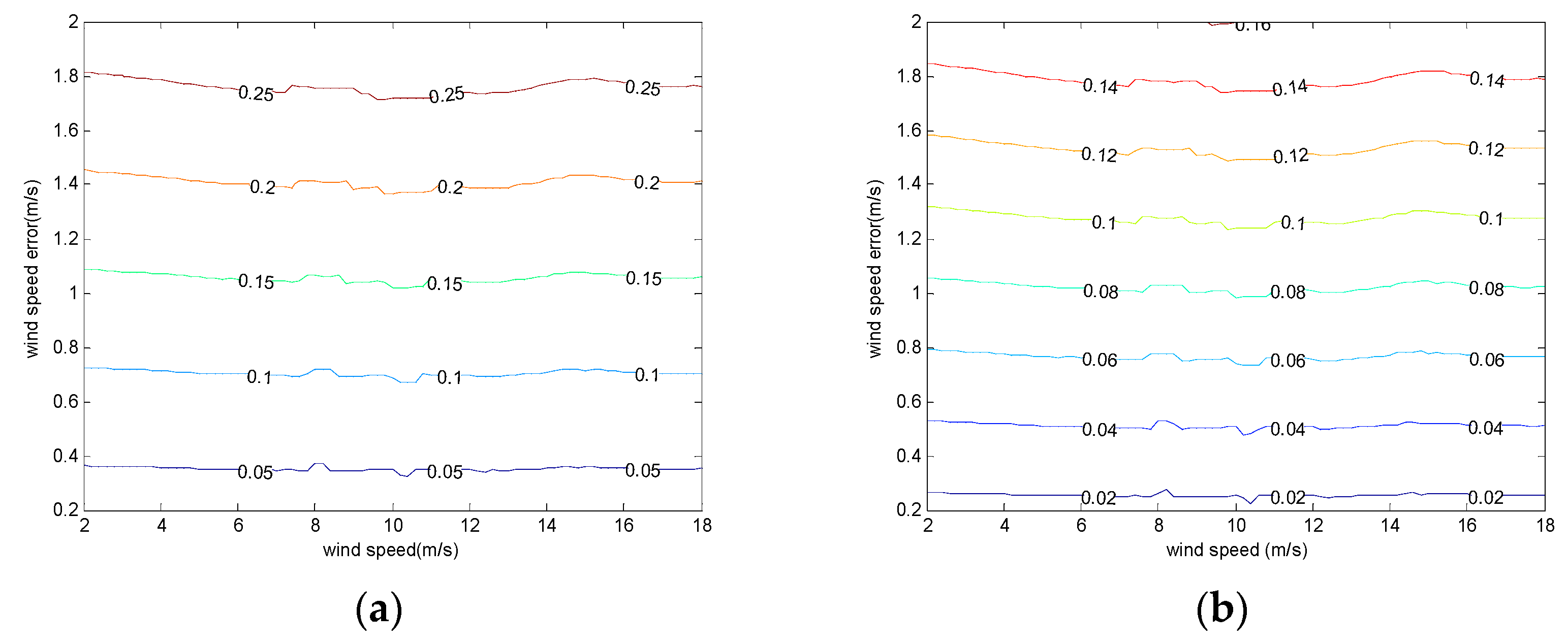
Figure 1.
Surface Doppler shift errors due to different wind speed errors in the downwind direction: (a) received and transmitted in horizontal polarization (HH polarization); (b) received and transmitted in vertical polarization (VV polarization).
Figure 1.
Surface Doppler shift errors due to different wind speed errors in the downwind direction: (a) received and transmitted in horizontal polarization (HH polarization); (b) received and transmitted in vertical polarization (VV polarization).
Figure 2.
Surface Doppler shift errors due to different wind speed errors in the upwind direction: (a) HH polarization; (b) VV polarization.
Figure 2.
Surface Doppler shift errors due to different wind speed errors in the upwind direction: (a) HH polarization; (b) VV polarization.
Figure 3.
Surface current velocity errors due to different wind speed errors in the downwind direction: (a) HH polarization; (b) VV polarization.
Figure 3.
Surface current velocity errors due to different wind speed errors in the downwind direction: (a) HH polarization; (b) VV polarization.
Figure 4.
Surface current velocity errors due to different wind speed errors in the upwind direction: (a) HH polarization; (b) VV polarization.
Figure 4.
Surface current velocity errors due to different wind speed errors in the upwind direction: (a) HH polarization; (b) VV polarization.
Figure 5.
Surface Doppler shift errors due to different wind direction errors: (a) HH polarization; (b) VV polarization.
Figure 5.
Surface Doppler shift errors due to different wind direction errors: (a) HH polarization; (b) VV polarization.
Figure 6.
Surface current velocity errors due to different wind direction errors: (a) HH polarization; (b) VV polarization.
Figure 6.
Surface current velocity errors due to different wind direction errors: (a) HH polarization; (b) VV polarization.
Figure 7.
Dual-frequency Doppler scatterometer (DfDopScat) scanning geometry.
Figure 7.
Dual-frequency Doppler scatterometer (DfDopScat) scanning geometry.
Figure 8.
Measurement principle: (a) pulse pair phase difference; (b) current vectors are estimated by combining multiple (2–4) radial velocity measurements.
Figure 8.
Measurement principle: (a) pulse pair phase difference; (b) current vectors are estimated by combining multiple (2–4) radial velocity measurements.
Figure 9.
Observation geometry of the pencil beam rotating scatterometer: (a) three-dimensional view; (b) different azimuth angle relations.
Figure 9.
Observation geometry of the pencil beam rotating scatterometer: (a) three-dimensional view; (b) different azimuth angle relations.
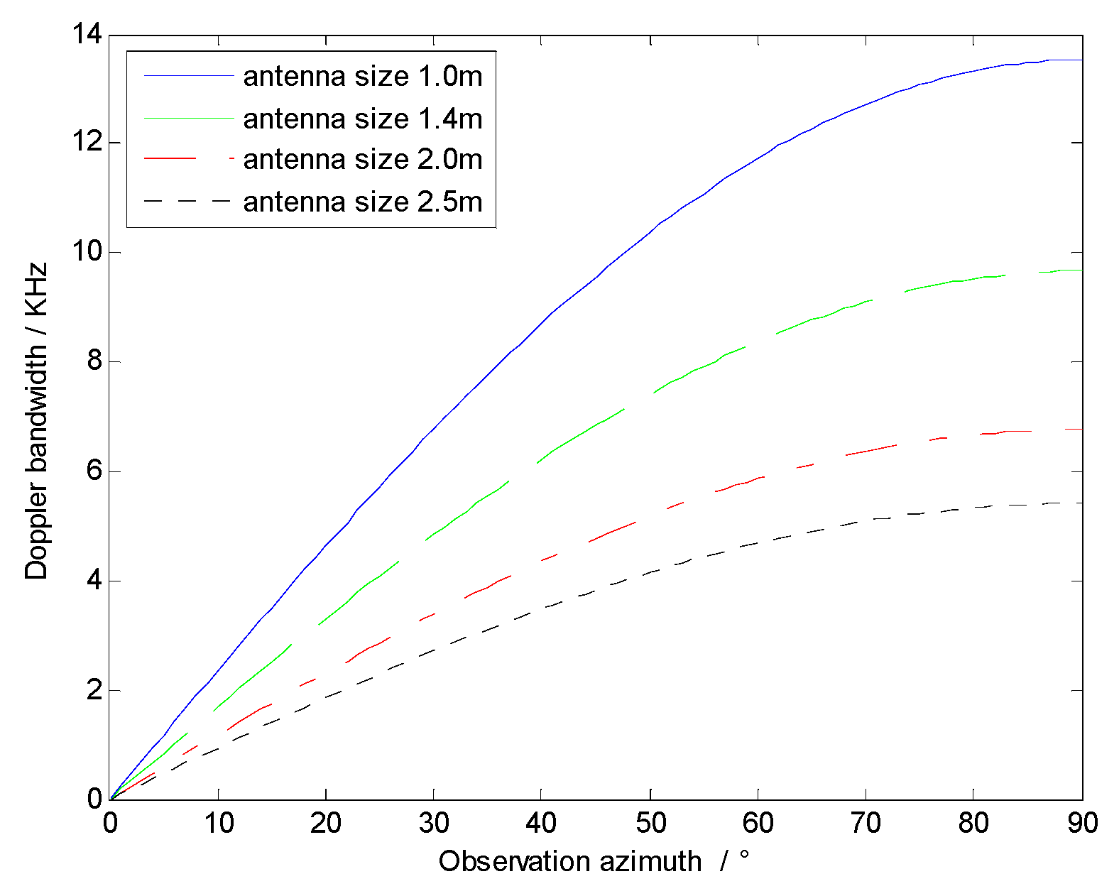
Figure 10.
Doppler bandwidths in different observation azimuths with different antenna sizes.
Figure 10.
Doppler bandwidths in different observation azimuths with different antenna sizes.
Figure 11.
The relationship between the pulse repetition frequency (PRF) and spatial decorrelation in different observation azimuths.
Figure 11.
The relationship between the pulse repetition frequency (PRF) and spatial decorrelation in different observation azimuths.
Figure 12.
The modified pulse sequence.
Figure 12.
The modified pulse sequence.
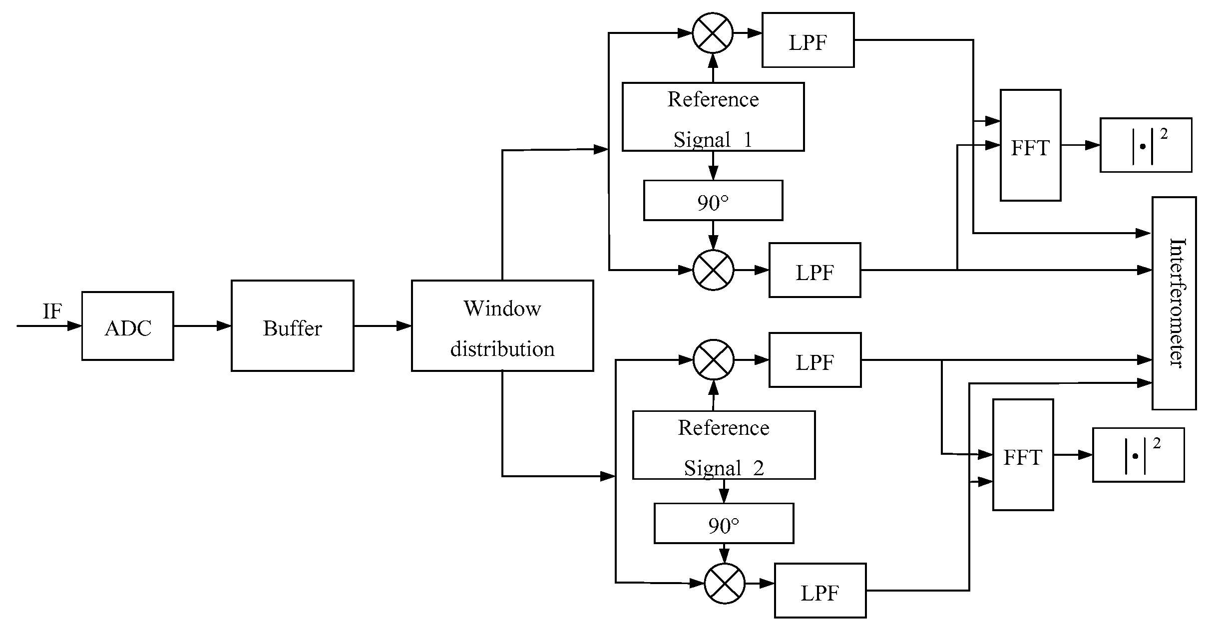
Figure 13.
Diagram of signal processing.
Figure 13.
Diagram of signal processing.
Figure 14.
End-to-end system simulation model diagram.
Figure 14.
End-to-end system simulation model diagram.
Figure 15.
Current velocity components Std with PRF for a wind speed of 7 m/s and a wind direction of 90°: (a) along-track direction; (b) cross-track direction.
Figure 15.
Current velocity components Std with PRF for a wind speed of 7 m/s and a wind direction of 90°: (a) along-track direction; (b) cross-track direction.
Figure 16.
Surface current velocity components Std with bandwidths for a wind speed of 7 m/s and a wind direction of 90°: (a) along-track direction; (b) cross-track direction.
Figure 16.
Surface current velocity components Std with bandwidths for a wind speed of 7 m/s and a wind direction of 90°: (a) along-track direction; (b) cross-track direction.
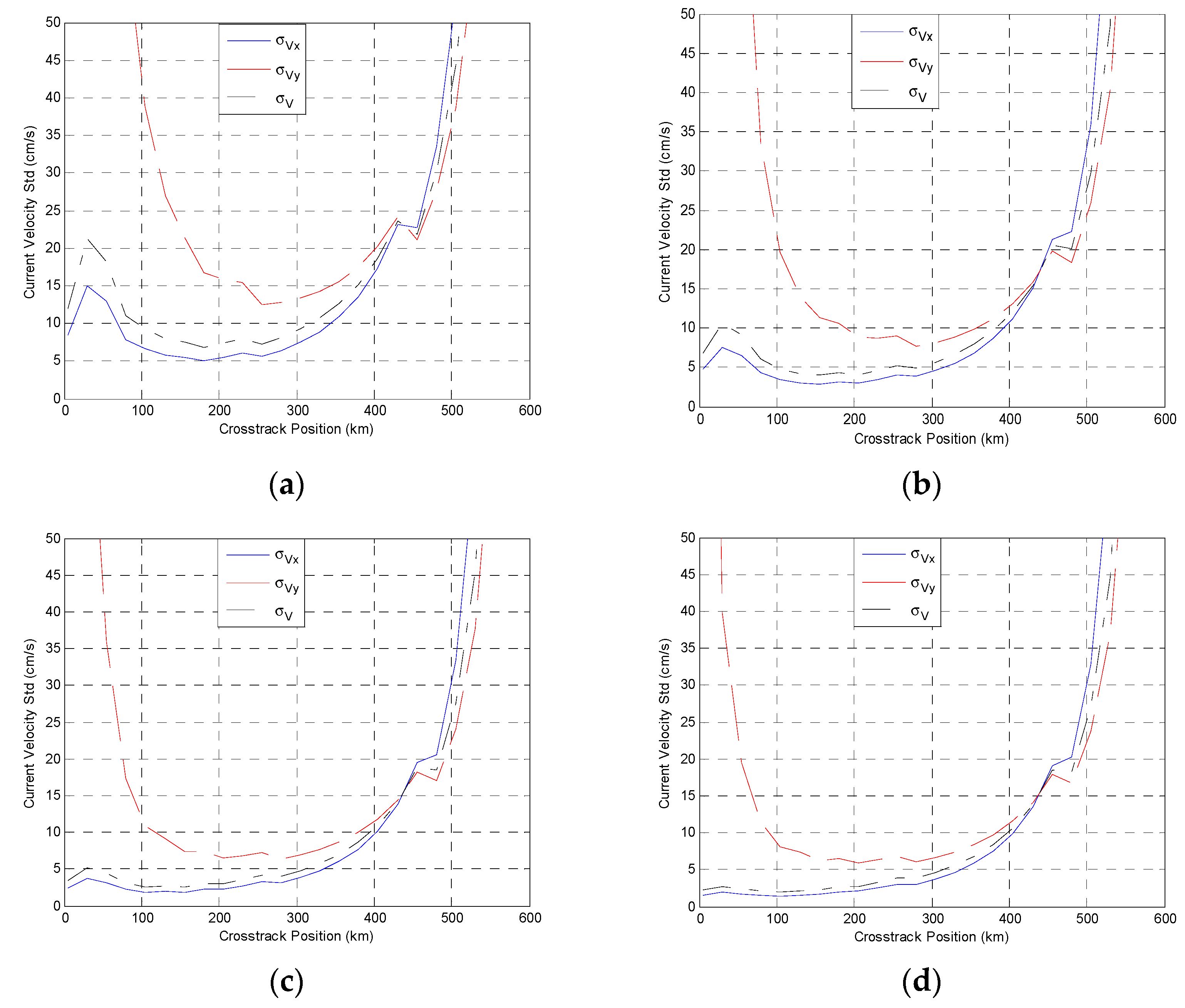
Figure 17.
Surface current velocity components Std in line-of-sight, cross-track, and along-track directions with a wind direction of 90°: (a) U = 4 m/s; (b) U = 7 m/s; (c) U = 14 m/s; (d) U = 21 m/s.
Figure 17.
Surface current velocity components Std in line-of-sight, cross-track, and along-track directions with a wind direction of 90°: (a) U = 4 m/s; (b) U = 7 m/s; (c) U = 14 m/s; (d) U = 21 m/s.
Figure 18.
The value of with different wind speeds: (a) comparison of between DopScat and a traditional fan-beam scatterometer; (b) comparison of between DopScat and a traditional pencil-beam scatterometer.
Figure 18.
The value of with different wind speeds: (a) comparison of between DopScat and a traditional fan-beam scatterometer; (b) comparison of between DopScat and a traditional pencil-beam scatterometer.
Figure 19.
Current velocity components Std with PRF for a wind speed of 7 m/s and a wind direction of 90°: (a) along-track direction; (b) cross-track direction.
Figure 19.
Current velocity components Std with PRF for a wind speed of 7 m/s and a wind direction of 90°: (a) along-track direction; (b) cross-track direction.
Figure 20.
Surface current velocity components Std with bandwidths for a wind speed of 7 m/s and a wind direction of 90°: (a) along-track direction; (b) cross-track direction.
Figure 20.
Surface current velocity components Std with bandwidths for a wind speed of 7 m/s and a wind direction of 90°: (a) along-track direction; (b) cross-track direction.
Figure 21.
Surface current velocity components Std in line-of-sight, cross-track, and along-track direction: (a) U = 4 m/s; (b) U = 7 m/s; (c) U = 14 m/s; (d) U = 21 m/s.
Figure 21.
Surface current velocity components Std in line-of-sight, cross-track, and along-track direction: (a) U = 4 m/s; (b) U = 7 m/s; (c) U = 14 m/s; (d) U = 21 m/s.
Figure 22.
Incidence angle and observation azimuth measurement errors caused by satellite attitude determinations: (a) incidence angle error; (b) observation azimuth error.
Figure 22.
Incidence angle and observation azimuth measurement errors caused by satellite attitude determinations: (a) incidence angle error; (b) observation azimuth error.
Figure 23.
Satellite attitude and velocity determinations effects on current retrieval: (a) yaw; (b) pitch; (c) roll; (d) satellite velocity.
Figure 23.
Satellite attitude and velocity determinations effects on current retrieval: (a) yaw; (b) pitch; (c) roll; (d) satellite velocity.
Figure 24.
Effects of satellite attitude and velocity determinations on current velocity error.
Figure 24.
Effects of satellite attitude and velocity determinations on current velocity error.
Table 1.
Orbital parameters.
Table 1.
Orbital parameters.
| Earth Model | WGS-84 |
|---|
| Orbit Height | 520 km |
| Eccentricity | 0 |
| Orbit inclination | 97.45° |
| Satellite Velocity | 7606 m/s |
Table 2.
Main parameters of the Ku-band DopScat.
Table 2.
Main parameters of the Ku-band DopScat.
| Parameters | Value |
|---|
| Transmitted Power | 200 W |
| Carrier Frequency | 13.256 GHz |
| Carrier Wavelength | 2.26 cm |
| 3dB Azimuth Beamwidth | 0.96° |
| 3dB Range Beamwidth | 0.96° |
| Antenna Incidence Angle | 48° |
| Antenna Gain | 46 dB |
| Rotation Rate | 18.3 rpm |
| System Loss | 5 dB |
| System Temperature | 290 K |
Table 3.
Current field effective swaths of different current velocity Stds with different values of PRF.
Table 3.
Current field effective swaths of different current velocity Stds with different values of PRF.
| PRF (kHz)/Current Velocity Std (m/s) | 8.0 | 9.0 | 10.0 | 11.0 | 12.0 | 13.0 | 14.0 | 15.0 |
|---|
| 0.10 | 326 | 342 | 358 | 378 | 328 | 220 | - | - |
| 0.15 | 488 | 538 | 606 | 604 | 596 | 544 | 414 | - |
| 0.20 | 574 | 632 | 696 | 704 | 708 | 686 | 594 | 220 |
| 0.25 | 668 | 726 | 780 | 766 | 768 | 770 | 704 | 436 |
| 0.30 | 696 | 766 | 816 | 814 | 894 | 828 | 770 | 512 |
Table 4.
Current field effective swaths (current velocity Std of 0.15m/s) with different values of PRF.
Table 4.
Current field effective swaths (current velocity Std of 0.15m/s) with different values of PRF.
| PRF (kHz) | Duty Cycle | Current Field Effective Swath (km) |
|---|
| 8.0 | 24.42% | 488 |
| 9.0 | 21.22% | 538 |
| 10.0 | 18.03% | 606 |
| 11.0 | 14.83% | 604 |
| 12.0 | 11.63% | 596 |
| 13.0 | 8.43% | 544 |
| 14.0 | 5.24% | 414 |
| 15.0 | 2.04% | - |
Table 5.
Signal-to-noise ratio (SNR) with different bandwidths.
Table 5.
Signal-to-noise ratio (SNR) with different bandwidths.
| Bandwidth (MHz) | SNR_VV (dB) |
|---|
| 1.0 | 10.14 |
| 1.5 | 8.38 |
| 2.0 | 7.13 |
| 2.5 | 6.16 |
| 3.0 | 5.37 |
| 3.5 | 4.70 |
| 4.0 | 4.13 |
| 4.5 | 3.61 |
| 5.0 | 3.15 |
Table 6.
Current field effective swaths (current velocity Std of 0.15 m/s) with different bandwidths.
Table 6.
Current field effective swaths (current velocity Std of 0.15 m/s) with different bandwidths.
| Bandwidth (MHz) | Current Field Effective Swath (km) |
|---|
| 1.0 | 352 |
| 1.5 | 442 |
| 2.0 | 510 |
| 2.5 | 544 |
| 3.0 | 561 |
| 3.5 | 580 |
| 4.0 | 596 |
| 4.5 | 600 |
| 5.0 | 609 |
Table 7.
Current field effective swaths of different current velocity Stds in different wind speeds.
Table 7.
Current field effective swaths of different current velocity Stds in different wind speeds.
| Wind Speed (m/s)/Current Velocity Std (m/s) | 2 | 3 | 4 | 5 | 6 | 7 | 8 | 9 | 10 | 11 | 15 | 18 | 21 |
|---|
| 0.10 | - | - | - | - | 270 | 340 | 420 | 460 | 496 | 514 | 554 | 574 | 584 |
| 0.15 | - | - | 222 | 460 | 548 | 594 | 624 | 652 | 664 | 678 | 714 | 720 | 734 |
| 0.20 | - | 158 | 478 | 610 | 658 | 692 | 708 | 726 | 750 | 770 | 802 | 818 | 842 |
| 0.25 | - | 468 | 642 | 676 | 762 | 780 | 796 | 814 | 824 | 830 | 856 | 870 | 882 |
| 0.30 | - | 560 | 698 | 764 | 796 | 816 | 834 | 842 | 854 | 862 | 892 | 902 | 914 |
Table 8.
Main parameters of the Ka-band DopScat.
Table 8.
Main parameters of the Ka-band DopScat.
| Parameters | Value |
|---|
| Transmitted Power | 150 W |
| Carrier Frequency | 35.75 GHz |
| Carrier Wavelength | 0.84 cm |
| 3dB Azimuth Beamwidth | 0.42° |
| 3dB Range Beamwidth | 0.42° |
| Antenna Incidence Angle | 48° |
| Antenna Gain | 53.6 dB |
| Rotation Rate | 18.3 rpm |
| System Loss | 7 dB |
| System Temperature | 290 K |
Table 9.
Current field effective swaths of different current velocity Stds with different values of PRF.
Table 9.
Current field effective swaths of different current velocity Stds with different values of PRF.
| PRF (kHz)/Current velocity Std (m/s) | 7.0 | 8.0 | 9.0 | 10.0 | 11.0 | 12.0 | 13.0 | 14.0 | 15.0 | 16.0 |
|---|
| 0.05 | 358 | 414 | 452 | 500 | 550 | 592 | 636 | 642 | 650 | 660 |
| 0.10 | 550 | 618 | 682 | 748 | 790 | 854 | 872 | 858 | 874 | 894 |
| 0.15 | 602 | 678 | 750 | 812 | 866 | 914 | 954 | 982 | 986 | 982 |
| 0.20 | 616 | 704 | 782 | 856 | 908 | 960 | 1004 | 1034 | 1048 | 1040 |
Table 10.
Current field effective swaths (current velocity Std of 0.05 m/s) with different values of PRF.
Table 10.
Current field effective swaths (current velocity Std of 0.05 m/s) with different values of PRF.
| PRF (kHz) | Duty Cycle | Current Field Effective Swath (km) |
|---|
| 7.0 | 39.81% | 358 |
| 8.0 | 38.36% | 414 |
| 9.0 | 36.90% | 452 |
| 10.0 | 35.45% | 500 |
| 11.0 | 34.00% | 550 |
| 12.0 | 32.54% | 592 |
| 13.0 | 31.09% | 636 |
| 14.0 | 29.63% | 640 |
| 15.0 | 28.18% | 650 |
| 16.0 | 26.72% | 660 |
Table 11.
Current field effective swaths (current velocity Std of 0.05 m/s) with different bandwidths.
Table 11.
Current field effective swaths (current velocity Std of 0.05 m/s) with different bandwidths.
| Bandwidth (MHz) | Current Field Effective Swath (km) |
|---|
| 2.0 | 532 |
| 2.5 | 562 |
| 3.0 | 586 |
| 3.5 | 608 |
| 4.0 | 622 |
| 4.5 | 630 |
| 5.0 | 650 |
| 5.5 | 654 |
| 6.0 | 660 |
Table 12.
Current field effective swaths of different current velocity Stds in different wind speeds.
Table 12.
Current field effective swaths of different current velocity Stds in different wind speeds.
| Wind Speed (m/s)/Current Velocity Std (m/s) | 2 | 3 | 4 | 5 | 6 | 7 | 8 | 9 | 12 | 15 | 18 |
|---|
| 0.05 | - | - | - | 376 | 560 | 660 | 706 | 738 | 784 | 790 | 766 |
| 0.10 | - | 272 | 602 | 758 | 842 | 894 | 920 | 944 | 976 | 982 | 990 |
| 0.15 | - | 640 | 830 | 896 | 942 | 982 | 1006 | 1028 | 1058 | 1060 | 1048 |
| 0.20 | 468 | 750 | 904 | 978 | 1008 | 1038 | 1068 | 1080 | 1096 | 1100 | 1107 |


