Abstract
Cloud removal is a prerequisite for the application of Landsat datasets, as such satellite images are invariably contaminated by clouds. Clouds affect the transmission of radiation signal to different degrees because of their different thicknesses, shapes, heights and distributions. Existing methods utilize pixel replacement to remove thick clouds and pixel correction techniques to rectify thin clouds in order to retain the land surface information in contaminated pixels. However, a major limitation of these methods refers to their deficiency in retrieving land surface reflectance when both thick clouds and thin clouds exist in the images, as the two types of clouds differ in the transmission of radiation signal. As most remotely sensed images show rather complex cloud contamination patterns, an efficient method to alleviate both thin and thick cloud effects is in need of development. To this end, the paper proposes a new method to rectify cloud contamination based on the cloud detection of iterative haze-optimized transformation (IHOT) and the cloud removal of cloud trajectory (IHOT-Trajectory). The cloud trajectory is able to take consideration of signal transmission for different levels of cloud contamination, which characterizes the spectral response of a certain type of land cover under increasing cloud thickness. Specifically, this method consists in four steps. First, the cloud thicknesses of contaminated pixels are estimated by the IHOT. Second, areas affected by cloud shadows are marked. Third, cloud trajectories are fitted with the aid of neighboring similar pixels under different cloud thickness. Last, contaminated areas are rectified according to the relationship between the land surface reflectance and the IHOT. The experimental results indicate that the proposed approach is able to effectively remove both the thin and thick clouds and erase the cloud shadows of Landsat images under different scenarios. In addition, the proposed method was compared with the dark object subtraction (DOS), the modified neighborhood similar pixel interpolator (MNSPI) and the multitemporal dictionary learning (MDL) methods. Quantitative assessments show that the IHOT-Trajectory method is superior to the other cloud removal methods overall. For specific spectral bands, the proposed method performs better than other methods in visible bands, whereas it does not necessarily perform better in infrared bands.
1. Introduction
Landsat data have been widely employed to investigate the Earth’s surface in applications such as urbanization, hazard monitoring, deforestation, and human-environment interactions as results of land use and land cover change [1,2,3,4,5]. One remaining issue of the Landsat images is that they are invariably contaminated by clouds, which significantly affect the electromagnetic signal transmission in the production of images [3,6,7,8,9]. Thus, the effective detection and removal of the cloud contamination are critical steps before the usage of Landsat imagery [3,10,11,12].
Many efforts have been devoted to alleviate the consequence of cloud contamination. The existing correction methods differ as the two types of clouds, thick clouds and thin clouds, affect the application of images in different ways. On the one hand, thick clouds block the majority of radiation from the land surface; and pixel substitution is the only way to remedy the information loss [13]. Zhu et al. [14] and Cheng [15] made effective attempts at substituting the clouded pixels with the spatiotemporal information derived from their neighboring similar pixels. Li et al. [16] further introduced a multi-temporal dictionary-learning approach to improve the effectiveness of the substitution process. These methods, however, require a significant portion of clear neighboring pixels as a prerequisite for restoration. In reality, it is very common that thick clouds and thin clouds both exist in a scene of a remotely sensed image. The existence of thin cloud will lead to a significant bias of the substitution process or a waste of the land surface information under the thin cloud. On the other hand, thin clouds (including hazes) manifest a certain degree of transparency and can be removed by very different atmospheric correction (AC) techniques [17]. In general, these techniques can be grouped into two categories: absolute AC and scene-based AC [18]. Absolute AC techniques are effective in resolving thin cloud contamination; however, they require auxiliary datasets about the regional atmospheric conditions over a time span, which are usually difficult to obtain [17]. Scene-based AC techniques consider cloud thickness as a parametric input of the correction process. The cloud thickness is commonly estimated by haze optimized transformation (HOT) [19] because of its robustness and simplicity [20,21,22,23,24]. Incorporated in the dark object substitution (DOS) model, the HOT-based AC techniques have been adopted for Landsat Thematic Mapper (TM) data as well as high-resolution satellite data [19]. One issue of the HOT is the over- and under-correction errors that affect the correction accuracy [19]. The DOS model also lacks the capability to recognize and eliminate the multiplicative effect of thin clouds [17]; and this deficiency has been later alleviated by the visual cloud point (VCP) method [25]. Such methods, however, are flawed in that (1) the bright surface is overcorrected because of the spectral confusion between the bright surface and clouds, and that (2) it is unable to tackle the contamination effect of thick clouds. Other cloud removal methods were made including attempts at machine learning through extracting multitemporal information [16,26,27] even though differences in phenology and land types may lead to failed learning.
Recently, a new method, referred to as the iterative haze optimized transformation (IHOT) technique, has been proposed to estimate the cloud thickness [28]. This method uses a corresponding clear image as a secondary dataset and applies an iterative regression process among the top of atmosphere (TOA) reflectance of the clear image, the TOA reflectance of the clouded image, and their difference in the TOA to characterize the haze contamination in the Landsat images. This method can distinguish clouds correctly from the bright surface and accurately derive cloud thickness. In addition, the concept of “cloud trajectory” has been proposed to characterize the spectral response of a certain type of land cover under increasing cloud thickness [19]. It also indicates that all cloud trajectories extend and intersect at a point, termed the “cloud point,” that only contains pure cloud spectrum without land surface information. However, cloud trajectory has been rarely employed for the purpose of cloud removal. In this paper, we propose a novel method to rectify clouded pixels by fitting the cloud trajectory with the aid of the IHOT. This method, termed the IHOT-trajectory method, can simultaneously remove thick clouds and thin clouds in an effective manner.
2. Methodology
As the reflectance of the clouds is usually larger than the energy attenuation during the signal transmission, the measured TOA reflectance of the land cover increases with the increase of the cloud thickness. This effect can be characterized by the cloud trajectory as a relationship between cloud thickness and TOA reflectance [19], as shown in Figure 1. Specifically, if the land cover is contaminated by clouds, the TOA reflectance in a band (i.e., Figure 1) displays a mathematical relationship with cloud thickness (i.e., Figure 1). The cloud trajectory for each land cover is able to take the signal transmission into consideration, including not only the additive reflectance from the clouds but also the energy attenuation when solar radiation passes through clouds. The cloud trajectory has two other distinct features. First, each type of land cover has a unique cloud trajectory; second, all these cloud trajectories of various land cover types culminate in a point, called the “cloud point,” which represents pure cloud spectra without land cover reflectance [19]. The rationale of the proposed cloud removal method is as follows: (1) establish the cloud trajectories of clouded pixels based on their spectral characteristics and cloud thickness; and (2) retrieve the clear pixels based on the cloud trajectories. The flowchart of the process, comprised of four major steps, is shown in Figure 2.
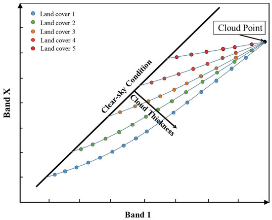
Figure 1.
Illustration of the cloud trajectory.
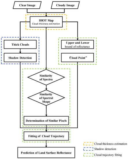
Figure 2.
Flowchart of the proposed method.
2.1. Cloud Thickness Estimation
The first step of the method is to estimate the cloud thickness using a recently developed IHOT algorithm [28]. This step requires a clear image of the study region as a secondary data to complement the clouded image. Then, multivariate regression models are established among the TOA reflectance of the clear image, the TOA reflectance of the clouded image, and their difference in the TOA in an iterative manner [28]. This improved IHOT algorithm ensures the large suppression of the land surface information and, thus, the effective extraction of the cloud information. The IHOT map is then generated, showing the spatial distribution of cloud thickness in terms of the IHOT index.
2.2. Shadow Detection
An additional source of contamination is the shadow effect, referring to the attenuated solar radiation on unclouded pixels induced by thick cloud shadows. The shadow effect will largely affect the accuracy of the restoration as the shadowed pixels may be erroneously used for cloud trajectory fitting in a follow-up process. As the shadow effect is mostly induced by thick clouds, a threshold of the IHOT index (IHOTThickClouds) is employed to demarcate thick clouds, as shown in Equation (1).
where IHOTcr and σcr are the average value and standard deviation of the IHOT index from the clear image. As there is a geometric similarity between the thick clouds and their shadows, we have adopted an object-based shadow detection method [9] to retrieve the shadows. This method contains two steps. First, the flood-fill combined with near infrared (NIR) band is applied to select potential shadow areas. Second, the view angle of the satellite sensor and the illuminating angle are used to determine the geographical relationships between clouds and their shadows. In this paper, we modify the second step by taking thick clouds as an input to match the shadows. The shadow areas can be effectively identified by matching the shape of the clouds.
2.3. Cloud Trajectory Fitting
The impact of increasing cloud optical depth on the reflectance of a given land cover can be characterized by a ‘cloud trajectory’ in spectral space [19]. Both the additive radiometric effect and energy attenuation effect of clouds can be characterized by the cloud trajectory as a relationship between cloud thickness and TOA reflectance, as shown in Figure 3. Therefore, the basic concept of cloud removal is to fit each unique cloud trajectory for each clouded pixel and migrate it back along the trajectory to the clear sky condition. This cloud trajectory fitting involves two steps. First, the general direction of the cloud trajectory is captured by setting the cloud point [19] as the end of the trajectory. To ensure the accuracy of the cloud trajectory, the second step searches for a series of similar clouded pixels with cloud thinner than that of the target pixel. By combining the cloud point and a series of similar clouded pixels, the cloud trajectory is constructed and can be applied for cloud removal.
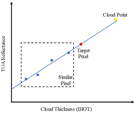
Figure 3.
Illustration for the cloud trajectory fitting.
2.3.1. Determining Cloud Point
As shown in Figure 1, all cloud trajectories intersect at the cloud point with only cloud signals. Thus, the first step for fitting the cloud trajectories is to retrieve the cloud point. The cloud point is obtained by calculating the intersection of the upper and lower bounds of the cloud trajectories by linear regressions [25]. Specifically, the IHOT of the clouded image is sliced into evenly distributed intervals, and the lower-bound and upper-bound of TOA reflectance value of histogram in each slice are found. Considering the unstableness of the minimum and the maximum value, a parameter, “p” (usually 0.02), and (1 − p) are chosen as the lower-bound and upper-bound values, respectively [25]. The trajectories need to be further calibrated as their forms are not exactly linear [19].
2.3.2. Retrieving Similar Clouded Pixels
To ensure the accuracy of the cloud trajectory fitting, the second step searches for a series of similar pixels with different cloud thicknesses. The similar pixels share the similar land surface reflectance and their TOA reflectance vary with only cloud thickness. In this search process, two types of pixels should be excluded: (1) the cloud shadows, as described in Section 2.2 and (2) the clouds thicker than that of the target pixel, as they contain less land cover information. Therefore, the search for similar clouded pixels is focused on the pixels with clouds thinner than that of the target pixel. The search range is a local window centered at the target pixel; and the search radius increases until qualified similar pixels are identified. The criterion is that at least one similar pixel should be found for each IHOT bin with an interval of 0.01. This is to ensure that the searched similar pixels are able to be as evenly distributed along with cloud trajectories, which assists in stabilizing the linear fitting of cloud trajectory. The two similarity measurements, namely, the spectral similarity and the spectral shape similarity, are applied to identify similar pixels. The illustration of such a process is shown in Figure 4. Since the spectra of blurry pixels in the clouded image may be confounded by the land surface [15], it is not practical to apply the spectral similarity directly to the clouded image. Thus, the secondary clear image of the corresponding region is used to search for similar pixels. Although images acquired at different times usually have some changes under different atmospheric or seasonal conditions, the relative positions of similar pixels generally are coincident in different seasons [14]. Thus, the spectral similarity of the correlation coefficient r of the clear image is calculated by Equation (2).
where Rtcri and Rcri denote the TOA reflectance of band i for a target pixel and that of its similar pixel under a clear sky, respectively; and denote the average of the TOA reflectance of all bands for the target pixel and that of its similar pixel under a clear sky, respectively; and n is the number of bands of the Landsat sensor at a 30-m resolution, which is 6 for Landsat TM/ETM+ and 7 for Landsat OLI. The threshold is set at 0.99 to strictly identify similar pixels. Such a measurement is reasonable based on the fact that similar pixels have a similar temporal change trend from the clear to clouded conditions [14,15]. However, there are still some similar pixels with the temporal change different from that of the target pixel, possibly induced by land cover change. Such similar pixels need to be further removed. The spectral shape similarity is then used to further qualify the similar pixels. Because the spectral shape of clouded pixels can be largely maintained, the clouded image is also used for the search process. The continuum removal is a useful tool to describe the spectral shape of the land surface. Thus, the correlation coefficient r’ based on the spectrum’s continuum removal is introduced to calculate the spectral shape similarity between the target pixel and its neighboring pixel at the time of the clouded image, as shown in Equation (3).
where Dti and Dci denote results of the continuum removal of band i for a target pixel and its potential similar one, and and denote the average of the results of continuum removal for the target pixel and its potential similar pixel. The threshold is always greater than 0.98. As a result, Equation (3) identifies the pixels sharing similar spectral characteristics and temporal change with the target pixel in the clouded image. The spectral similarity is a critical index in the selection process, as thick clouds reduce the differences of the spectral shapes among a variety of land surfaces. The criterion of searching for the spectral shape similarity has to be less strict (i.e., the lower threshold is set to 0.5) in order to include more similar pixels. Under the two selection criteria, pixels with different phenologies or land cover features in the clouded images can be removed; and similar clouded pixels can be selected for the construction of the cloud trajectories.
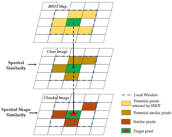
Figure 4.
Illustration of the process searching for similar pixels.
2.3.3. Cloud Trajectory Fitting
After the cloud point and similar clouded pixels are identified, the cloud trajectory for each clouded pixel can be constructed. For each band, the cloud trajectory can be described by a linear regression model, as shown in Equation (4).
where Rsi is the TOA reflectance of band i for the qualified similar clouded pixel, βi is the coefficient of IHOT, ci is a constant, and εi is the residual of the regression.
2.4. Cloud Removal
Based on the constructed cloud trajectories, the IHOT of the target clouded pixel as a function of its TOA reflectance can be described by Equation (5).
where Rti is the TOA reflectance of band i for the target pixel to be corrected, βi is the coefficient of IHOT, and ci is a constant. Based on the cloud trajectories for each band, all clouded pixels can then be corrected by Equation (6).
where R′ti is the corrected TOA reflectance in band i of the target clouded pixel, Rti is that of the uncorrected TOA reflectance, and IHOTcr is the average IHOT value in the clear image. It is also worth mentioning that the shadowed pixels can also be corrected by Equation (6).
For heavily contaminated pixels, land cover information may be obscured by thick clouds. Thus, the temporal change between the clear image and the clouded image are derived to restore the lost texture information. Here, we used the following criterion (Equation (7)) to determine the heavily cloud contaminated pixels).
where σcr is the standard deviation of the IHOT map for the clear image. For the heavily contaminated pixels, temporal changes of the similar pixels are considered in the correction procedure by Equation (8).
where R″ti is the corrected TOA reflectance of band i for the target pixel under heavily thick clouds, is the average TOA reflectance of band i derived from the similar pixels of the target in the clouded image, Rtcri is the TOA reflectance of band i for the corresponding pixel in the clear image, and is the average TOA reflectance of band i derived from the pixels similar to the target pixel in the clear image.
3. Experiment
3.1. Study Area and Data
To test the proposed IHOT-Trajectory method’s performance on complex cloud contamination patterns, a study area (37°N, 117°E) including a variety of land covers (cropland, vegetation, urban area, and bare soil) was selected and the corresponding Landsat images (Path 122, Row 34) were collected. As shown in Figure 5 and Figure 6, the proposed method was tested using the images with different phenologies. This experiment aims to examine whether a single clear-sky image can be used for multiple clouded images for the proposed methodology, with the consideration that limited amounts of clear-sky data are available. Table 1 shows the detailed information of the tested Landsat images. Specifically, a single clear image captured in March 2014 was used as the secondary image for the IHOT calculation and cloud removal of the cloud-contaminated images acquired in April 2014 and June 2013. Large phenological differences can be observed between the clear image and the clouded images. In the experiments, the proposed method was compared with a classical thin cloud removal method, the dark object subtraction (DOS) combined with HOT and IHOT as HOT-DOS [19] and IHOT-DOS. We also compared the IHOT-Trajectory with two cutting-edge cloud removal methods visually and quantitively, namely the modified neighborhood similar pixel interpolator (MNSPI) [14] and the multitemporal dictionary learning (MDL) [26]. The former is especially widely used for thick cloud removal while the latter has recently been developed based on sparse-representation. It is difficult to acquire the ground truth data for validating the cloud removal results. As an alternative, reference images captured in the similar seasons but different years were selected for the validation of the cloud removal results (Table 1). Such a method is reasonable because minor phenological and land cover changes occurred between the two acquisition dates within three years. However, identifying such cloud-free images for references is still very challenging, especially for a large area. For this reason, assessments were only performed in the sub-areas where cloud-free data are available for reference (Figure 5b,c and Figure 6b,c).
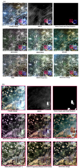
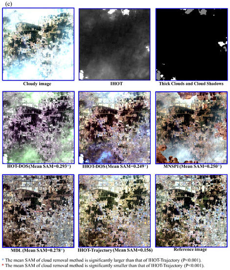
Figure 5.
Cloud removal of Landsat image (122/34) acquired at 22 April 2014 (a) whole image; (b) enlarged images of the subset area; (c) enlarged images of the subset area.
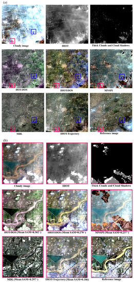
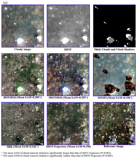
Figure 6.
Cloud removal of Landsat image (122/34) acquired at 6 June 2013 (a) whole image; (b) enlarged images of the subset area; (c) enlarged images of the subset area.

Table 1.
Summary of the Landsat scenes acquired in different seasons (path/row: 122/34; size: 3545 × 3239).
3.2. Cloud Removal Results
As shown in Figure 5 and Figure 6, the IHOT-Trajectory method simultaneously removed both thick clouds and thin clouds. The land cover reflectance affected by the shadow effect was also restored. Moreover, both clouded images with different phenologies were correctly restored, indicating the IHOT-Trajectory is insensitive to the phenology difference between the secondary clear image and the clouded image. Even though the acquisition dates of the clouded images were in April 2014 and June 2013, respectively, the secondary image acquired in March 2013 still worked effectively. Visual evaluations of the subsets of cloud removal results were shown in Figure 5b,c and Figure 6b,c. In Figure 5b,c, cropland, bare soil, industrial land and urban area were effectively recovered as well as their texture information. As shown in Figure 6b,c, the IHOT-Trajectory was also able to restore the cropland, urban and lake. In contrast, the HOT-DOS and IHOT-DOS were only limited to the removal of thin clouds and are not able to address the issues of thick clouds and shadows (Figure 5 and Figure 6). As the cloud contamination pattern is very complex with mixed clouds (Figure 5a), both the HOT-DOS and IHOT-DOS methods are ineffective in restoring the correct color of the land cover of green cropland, bare soil, and urban land. Since MNSPI can remove clouds only if there exist enough clear-sky neighboring similar pixels [14], here MNSPI performed poorly in a thick-clouded area for only hazy pixels were available. As shown in Figure 6b, the color of the impervious surface is largely biased. The MDL method had a better performance than MNSPI (Figure 5), whereas it hardly restored the correct phenology information of vegetation in the mountain area (Figure 5b) and cropland (Figure 5c). In general, MDL works poorly when there is large phenological difference between the secondary clear image and clouded image.
3.3. Quantitative Assessment of the Methods
Apart from visual validation, quantitative assessment was employed to evaluate the accuracy of the proposed method. Notably, identifying cloud-free images with phenological patterns matching the reference image was very challenging, especially over a large area. For this reason, assessments were only performed in the sub-areas where cloud-free data are available for reference (Figure 5b,c and Figure 6b,c). We assessed the quality of the cloud removal results by comparing with the subset of the reference images. Three indices were used for quantitatively describing the accuracy of the cloud removal result. The mean spectral angle mapper (SAM) was used for evaluating the overall performance of the cloud removal methods [29]. Spectral angle was calculated between the corrected spectrum and the reference spectrum. The correlation coefficient (r) and root mean square error (RMSE) were used for evaluating the cloud removal accuracy in each band. Meanwhile, paired T-tests were conducted to check whether the mean SAM and the absolute error of the proposed method were significantly smaller than those of other methods. As labeled in Figure 5 and Figure 6, mean SAM of cloud removal results by proposed method was significantly smaller than those of other methods. For visible spectral bands, the proposed method shows significant superiorities (lower RMSE and higher r) compared with other methods (Figure 7 and Figure 8). For infrared bands, the proposed method performed better than DOS-based methods, whereas not necessarily better than MNSPI and MDL (Figure 7 and Figure 8).
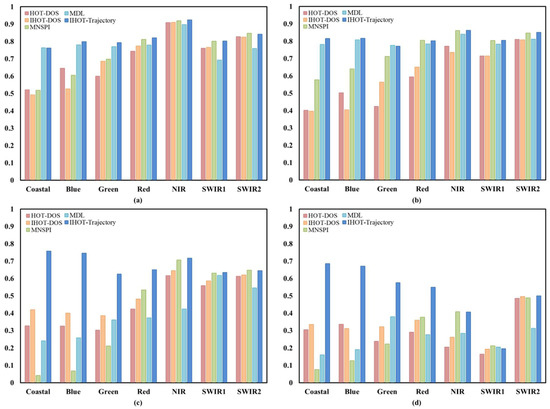
Figure 7.
Correlation coefficients (r) between the reference image and the restored image using haze optimized transformation-dark object subtraction (HOT-DOS), iterative haze-optimized transformation-DOS (IHOT-DOS), IHOT removal of cloud trajectory (IHOT-Trajectory), modified neighborhood similar pixel interpolator (MNSPI) and multitemporal dictionary learning (MDL). (a–d) correspond to r of Figure 5b,c and Figure 6b,c, respectively.
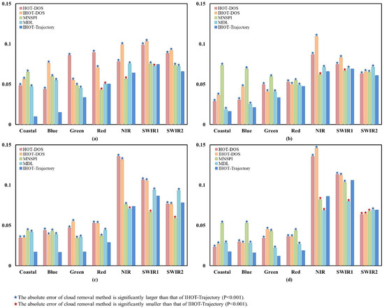
The results indicated the IHOT-Trajectory was able to overcome large phenological differences between the secondary clear image and the clouded images. In contrast, the DOS-based methods performed worst in most land covers. Because there always exist thick clouds, DOS-based methods quickly become ineffective in all spectral bands from visible to shortwave infrared (SWIR). The MNSPI method also performed quite poorly in complex cloud-contamination areas because of a strict requirement for clear similar pixels. Although MDL had a better performance than MNSPI and DOS in Figure 5, it showed considerable flaws in Figure 6. Possibly, large phenological differences between the secondary and clouded images influenced the accuracy of multi-dictionary learning. In summary, the IHOT-Trajectory method has the best performance in most spectral bands except for infrared bands. The least improvement in the infrared bands might be explained by two reasons. First, the atmospheric effect is relatively weak in the SWIR bands. Second, there are stronger non-linear effects in the relationship between IHOT and TOA reflectance in the SWIR bands.
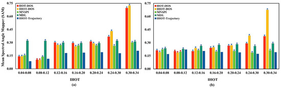
In order to further investigate the relationship between the cloud removal error and the cloud thickness, mean SAM values were calculated under different IHOT bins. As shown in Figure 9, the proposed method performed quite robustly and possessed high accuracy and stability as the IHOT value increased. It indicates that there is no obvious difference between the cloud removal errors on thick and thin clouds, although the removal of thick cloud is particularly treated with Equation (8) that is slightly different from Equation (6) used for the removal of relatively thin clouds. In contrast, the performance of the HOT-DOS and IHOT-DOS methods became increasingly worse as the cloud thickness increased because DOS methods require a transparent signal for cloud correction. For MNSPI and MDL, both of them also have stable performances as cloud thickness increases whereas their mean SAM values continuously maintain higher values.
4. Discussion and Conclusions
In this paper, we proposed a new cloud removal method by fitting the cloud trajectory with the aid of the IHOT algorithm. This method considers the signal transmission process and removes thick and thin clouds in Landsat imagery in an efficient manner. The method also eliminates the shadow effect and resolves the issue of information loss in images with complex cloud contamination patterns. Specifically, the cloud trajectories are established by searching for pixels with similar cloud thicknesses using the IHOT algorithm. This process enables the fitting of clouded pixels by a linear model. The application to the clouded images captured in different seasons confirms the efficiency and robustness of the proposed method, which outperforms other cloud removal methods, including the HOT-DOS, the IHOT-DOS, MNSPI and MDL. In addition, the proposed method is able to tolerate the phenological differences between the clouded image and the secondary clear image. This advantage further corroborates the effectiveness of pixel correction when seasonal dynamics is involved in the secondary data.
The method still has limitations. First, the IHOT-Trajectory is affected by a shadow detection error. Sometimes shadows are not successfully detected because of the strict object-based matching criteria in the shadow detection method employed [9]. The limitation caused by shadow mismatch can be remedied when more accurate shadow detection methods are developed in future. In addition, the threshold of thick cloud should be determined empirically, which could affect the cloud removal result. However, as the IHOT values of clear pixels are reasonably considered as normally distributed, correctly adjusting this parameter is not very difficult.
In conclusion, the proposed IHOT-Trajectory method introduces the cloud trajectory with the assistance of IHOT to remove thick, thin clouds and shadows simultaneously. As it can restore accurate reflectance, texture and phenology information for the clouded images with a variety of land covers, IHOT-Trajectory has potentials to make full use of the cloud-contaminated Landsat imagery that were generally wasted in previous applications. In terms of other comparable satellites, when their clear imagery datasets are available, IHOT-Trajectory could possibly be applied for cloud contamination removal.
Author Contributions
Conceptualization, X.C. (Xuehong Chen) and X.C. (Xiang Chen); Data curation, S.C.; Formal analysis, S.C. and M.S.; Funding acquisition, X.C. (Xuehong Chen), J.C., M.S. and W.Y.; Investigation, X.C. (Xin Cao); Methodology, S.C., X.C. (Xuehong Chen), J.C. and X.C. (Xin Cao); Project administration, J.C. and X.C. (Xihong Cui); Resources, J.C.; Supervision, X.C. (Xuehong Chen); Validation, X.C. (Xin Cao) and W.Y.; Visualization, S.C.; Writing—original draft, S.C.; Writing—review and editing, X.C., X.C., M.S. and X.C. (Xuehong Chen).
Funding
This research was supported by the National Key Research and Development Program of China (2017YFD0300201), State Key Laboratory of Earth Surface Processes and Resource Ecology, and CEReS Overseas Joint Research Program, Chiba University (No. CI16-101).
Conflicts of Interest
The authors declare no conflict of interest.
References
- Huang, C.; Goward, S.N.; Masek, J.G.; Thomas, N.; Zhu, Z.; Vogelmann, J.E. An automated approach for reconstructing recent forest disturbance history using dense Landsat time series stacks. Remote Sens. Environ. 2010, 114, 183–198. [Google Scholar] [CrossRef]
- Huang, C.; Thomas, N.; Goward, S.N.; Masek, J.G.; Zhu, Z.; Townshend, J.R.; Vogelmann, J.E. Automated masking of cloud and cloud shadow for forest change analysis using Landsat images. Int. J. Remote Sens. 2010, 31, 5449–5464. [Google Scholar] [CrossRef]
- Irish, R.R. Landsat 7 automatic cloud cover assessment. In Proceedings of the AeroSense 2000, Orlando, FL, USA, 24–28 April 2000; International Society for Optics and Photonics: Bellingham, WA, USA, 2000; pp. 348–355. [Google Scholar]
- Kennedy, R.E.; Cohen, W.B.; Schroeder, T.A. Trajectory-based change detection for automated characterization of forest disturbance dynamics. Remote Sens. Environ. 2007, 110, 370–386. [Google Scholar] [CrossRef]
- Vogelmann, J.E.; Tolk, B.; Zhu, Z. Monitoring forest changes in the southwestern United States using multitemporal Landsat data. Remote Sens. Environ. 2009, 113, 1739–1748. [Google Scholar] [CrossRef]
- Asner, G.P. Cloud cover in Landsat observations of the Brazilian Amazon. Int. J. Remote Sens. 2001, 22, 3855–3862. [Google Scholar] [CrossRef]
- Dozier, J. Spectral signature of alpine snow cover from the Landsat Thematic Mapper. Remote Sens. Environ. 1989, 28, 9–22. [Google Scholar] [CrossRef]
- Irish, R.R.; Barker, J.L.; Goward, S.N.; Arvidson, T. Characterization of the Landsat-7 ETM+ automated cloud-cover assessment (ACCA) algorithm. Photogramm. Eng. Remote Sens. 2006, 72, 1179–1188. [Google Scholar] [CrossRef]
- Zhu, Z.; Woodcock, C.E. Object-based cloud and cloud shadow detection in Landsat imagery. Remote Sens. Environ. 2012, 118, 83–94. [Google Scholar] [CrossRef]
- Arvidson, T.; Gasch, J.; Goward, S.N. Landsat 7’s long-term acquisition plan—An innovative approach to building a global imagery archive. Remote Sens. Environ. 2001, 78, 13–26. [Google Scholar] [CrossRef]
- Simpson, J.J.; Stitt, J.R. A procedure for the detection and removal of cloud shadow from AVHRR data over land. Geoscience and Remote Sensing. IEEE Trans. Geosci. Remote Sens. 1998, 36, 880–897. [Google Scholar] [CrossRef]
- Shen, H.; Li, H.; Qian, Y.; Zhang, L.; Yuan, Q. An effective thin cloud removal procedure for visible remote 418 sensing images. ISPRS J. Photogramm. Remote Sens. 2014, 96, 224–235. [Google Scholar] [CrossRef]
- Lu, D. Detection and substitution of clouds/hazes and their cast shadows on IKONOS images. Int. J. Remote Sens. 2007, 28, 4027–4035. [Google Scholar] [CrossRef]
- Zhu, X.; Gao, F.; Liu, D.; Chen, J. A modified neighborhood similar pixel interpolator approach for removing thick clouds in Landsat images. IEEE Geosci. Remote Sens. Lett. 2012, 9, 521–525. [Google Scholar] [CrossRef]
- Cheng, Q.; Shen, H.; Zhang, L.; Yuan, Q.; Zeng, C. Cloud removal for remotely sensed images by similar pixel replacement guided with a spatio-temporal MRF model. ISPRS J. Photogramm. Remote Sens. 2014, 92, 54–68. [Google Scholar] [CrossRef]
- Li, X.; Shen, H.; Zhang, L.; Zhang, H.; Yuan, Q.; Yang, G. Recovering quantitative remote sensing products contaminated by thick clouds and shadows using multitemporal dictionary learning. IEEE Trans. Geosci. Remote Sens. 2014, 52, 7086–7098. [Google Scholar]
- He, X.Y.; Hu, J.B.; Chen, W.; Li, X.Y. Haze removal based on advanced haze-optimized transformation (AHOT) for multispectral imagery. Int. J. Remote Sens. 2010, 31, 5331–5348. [Google Scholar] [CrossRef]
- Hasjimitsis, D.G.; Clayton, C.R.I.; Hope, V.S. An assessment of the effectiveness of atmospheric correction algorithms through the remote sensing of some reservoirs. Int. J. Remote Sens. 2004, 25, 3651–3674. [Google Scholar] [CrossRef]
- Zhang, Y.; Guindon, B.; Cihlar, J. An image transform to characterize and compensate for spatial variations in thin cloud contamination of Landsat images. Remote Sens. Environ. 2002, 82, 173–187. [Google Scholar] [CrossRef]
- Moro, G.D.; Halounova, L. Haze removal for high-resolution satellite data: A case study. Int. J. Remote Sens. 2007, 28, 2187–2205. [Google Scholar] [CrossRef]
- Olthof, I.; Pouliot, D.; Fernandes, R.; Latifovic, R. Landsat-7 ETM+ radiometric normalization comparison for northern mapping applications. Remote Sens. Environ. 2005, 95, 388–398. [Google Scholar] [CrossRef]
- Zhang, Y.; Guindon, B. Quantitative assessment of a haze suppression methodology for satellite imagery: Effect on land cover classification performance. IEEE Trans. Geosci. Remote Sens. 2003, 41, 1082–1089. [Google Scholar] [CrossRef]
- Zhang, Y.; Guindon, B.; Li, X. A robust approach for object-based detection and radiometric characterization of cloud shadow using haze optimized transformation. IEEE Trans. Geosci. Remote Sens. 2014, 52, 5540–5547. [Google Scholar] [CrossRef]
- Sun, L.; Latifovic, R.; Pouliot, D. Haze Removal Based on a Fully Automated and Improved Haze Optimized Transformation for Landsat Imagery over Land. Remote Sens. 2017, 9, 972. [Google Scholar]
- Liu, C.; Hu, J.; Lin, Y.; Wu, S.; Huang, W. Haze detection, perfection and removal for high spatial resolution satellite imagery. Int. J. Remote Sens. 2011, 32, 8685–8697. [Google Scholar] [CrossRef]
- Xu, M.; Jia, X.; Pickering, M.; Plaza, A.J. Cloud removal based on sparse representation via multitemporal dictionary learning. IEEE Trans. Geosci. Remote Sens. 2016, 54, 2998–3006. [Google Scholar] [CrossRef]
- Tahsin, S.; Medeiros, S.C.; Hooshyar, M.; Singh, A. Optical Cloud Pixel Recovery via Machine Learning. Remote Sens. 2017, 9, 527. [Google Scholar] [CrossRef]
- Chen, S.; Chen, X.; Chen, J.; Jia, P.; Cao, X.; Liu, C. An Iterative Haze Optimized Transformation for Automatic Cloud/Haze Detection of Landsat Imagery. IEEE Trans. Geosci. Remote Sens. 2016, 54, 2682–2694. [Google Scholar] [CrossRef]
- Xu, M.; Pickering, M.; Plaza, A.J.; Jia, X. Thin cloud removal based on signal transmission principles and spectral mixture analysis. IEEE Trans. Geosci. Remote Sens. 2016, 54, 1659–1669. [Google Scholar] [CrossRef]


© 2018 by the authors. Licensee MDPI, Basel, Switzerland. This article is an open access article distributed under the terms and conditions of the Creative Commons Attribution (CC BY) license (http://creativecommons.org/licenses/by/4.0/).