Article

Spatial Assessment of Water Quality with Urbanization in 2007–2015, Shanghai, China

1
Department of Geography, University of South Carolina, Columbia, SC 29208, USA
2
Georgia-Alabama Land Trust, Inc., Piedmont, AL 36272, USA
*
Author to whom correspondence should be addressed.
Remote Sens. 2018, 10(7), 1024; https://doi.org/10.3390/rs10071024
Submission received: 8 May 2018 / Revised: 14 June 2018 / Accepted: 25 June 2018 / Published: 27 June 2018

Abstract

:
Shanghai, as one of the megacities and economic centers of China, is facing critical water quality challenges. This study analyzed the impact of urbanization on the water quality in Shanghai, from 2007 to 2015, using remote sensing (RS) and geographic information system (GIS) techniques. Five measurements of water quality were employed: total discharged wastewater volume, general water quality levels, dissolved oxygen (DO), permanganate, and ammonia nitrogen. The impacts of urban land-use changes on water quality were examined. An urban index was extracted from satellite image classification and was used to quantify the anthropogenic activities. In the watershed level, unit watersheds were delineated from topography and stream segments. Results showed that the primary contributors of water quality degradation in Shanghai were DO and ammonia nitrogen. Both indicators expressed clear seasonal patterns that can be explained by agricultural activities and urbanization processes in Shanghai during the study period. Water quality was also regulated through water use policies. For example, the degraded water quality in suburban outskirts and improved water quality was achieved through the enforced wastewater discharge regulations in central Shanghai. Analytical findings provide spatially explicit information for governmental management on protecting water resources and controlling wastewater emissions, thus, improving the quality of living environments in this ever-growing megacity.

1. Introduction

Water is the most vital living prerequisite for mankind. China has been pressured by an enormous population, limited water resources [1,2], and water contamination issues [3,4]. Water pollution, especially, has attracted increasing attention since the 1990s [5] alongside China’s rapid economic development and urbanization process [6]. Shanghai, located downstream of the Yangtze River, is one of the economic centers and megacities of China. Shanghai has a remarkable population density and has been experiencing rapid social-economic development. The urbanization process in Shanghai accelerated since Chinese economic reform was initiated in 1978 [7,8]. Municipal sewage started to contribute significantly to the water environment and ecosystems, along with land development [9,10]. The geographical location of Shanghai potentially helps in accumulating more pollutants [7,8,9,10,11,12]. Meanwhile, Shanghai has the highest greenery coverage among all the cities in China, benefitting from the substantial amount of water volume [13]. The vegetation coverage, i.e., parks, forests, and grasslands, could improve surface and ground water quality [3,14].
Intensive studies of water pollution have been conducted using in situ sampling in water bodies [9,11,12]. Water samples were used to measure water quality indicators such as temperature, pH, and turbidity through physical-chemical experiments. Studies have identified various point- and non-point sources of water pollution and interwoven contributors, such as urbanization, industrialization, and agricultural activity [14,15,16,17,18,19]. With the widespread application of remote sensing (RS) and geographic information system (GIS) technologies, studies have shifted to a spatial and temporal perspective, such as mapping water resource distribution, modeling sewer networks, managing drinking water quality, and monitoring water pollution levels [13,20,21,22]. The Soil and Water Assessment Tool (SWAT) has been widely adopted as a powerful, watershed-based model that simulates the influence of both human and natural processes, such as land management, climate change, and agricultural activities [23]. Statistical methods, such as linear regression [24,25,26,27,28], have been used to evaluate relationships between water contamination levels and causal factors [23]. Urban land use types and changes have been analyzed and employed as indicators in investigating water quality, urban heat island, and other ecosystem questions [7,29,30,31,32,33,34,35]. For one of the fastest growing cities in economic development, population changes, and urban sprawling, satellite images provide a more accurate estimation in terms of real time monitoring [30]. Urbanization can be indicated by population density (using dasymetric models), industrial output, gross domestic product, etc. [7,29,30,31,32]. According to the Yearbook [13], Shanghai has a large number of migrants (close to 10 million, 40% of the total population of Shanghai). This floating population could cause bias in reflecting the urbanization in a spatiotemporal analysis [31]. Current literature has identified some major pollution sources from both human and natural environments [3,4,14]. Industrial wastewater, for example, is one of the most serious water pollution sources due to its high toxicity and untraceable characteristics [6,10]. The extensive use of pesticides and fertilizers is of grave concern for ground and surface water contamination with biological chemicals [28,36]. These influential factors in Shanghai urban ecosystems have not been thoroughly investigated and merit further study. For instance, in He et al.’s research [29], a land utility index was introduced concerning the utility of land types in any given study year, as well as the weight of land types. An analytic hierarchy process with an expert-consulting graded approach was applied. However, from the hydrogeological perspective, water quality analysis based on watersheds would be more appropriate than the administrative division, even at pixel level. Yin et al.’s study [7] used land use land cover (LULC) classification from satellite images as an urban indicator for water quality. However, using only one Landsat image to represent urban development is limited, let alone when the water quality data records could not match the image acquisition time. Applying an approach developed by Li et al. [14] to address water quality problems, this study explored long-term water sampling records within the study period of 2007–2015 using two satellite images to investigate the spatial-temporal variation of water quality and its relationships with land-use changes in the urban watershed of Shanghai.

2. Materials and Methodology
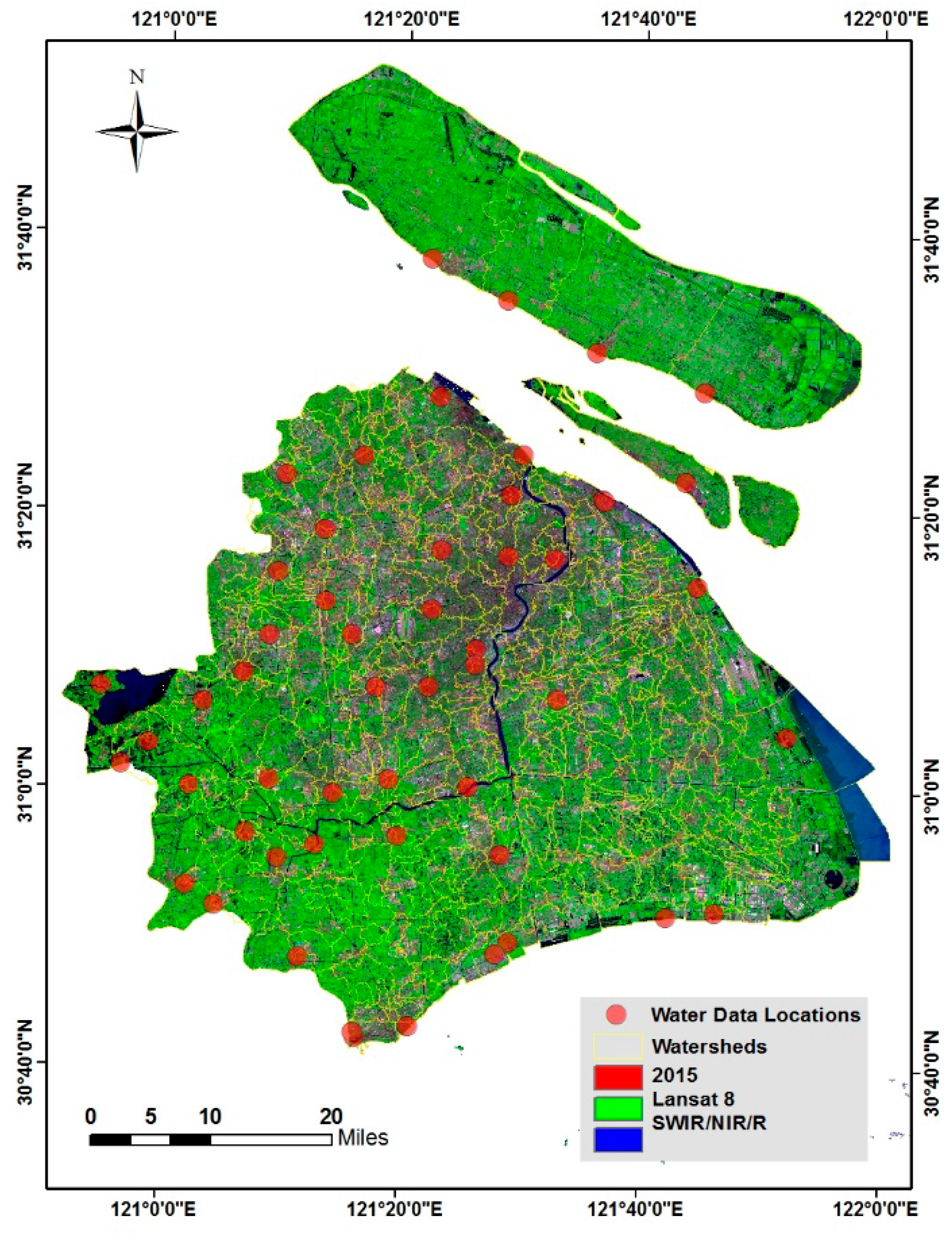
2.1. Study Area

The study area covers the city of Shanghai, which is composed of 16 urban districts, 210 suburban townships, and rural villages with a total area of 6341 km2 (Figure 1). Its population reached 24 million in 2015 [13]. Shanghai is located in the east end of the Yangtze River Delta alluvial plain and has a sophisticated water system. According to Shanghai Water Authority and Shanghai Municipal Bureau of Statistics (2011), there are 10 rivers and five lakes in Shanghai. Of these, Huangpu is the largest and the most famous due to its multiple functions, such as providing drinking water sources, transportation, flood prevention, fisheries, and tourism. Though there is adequate water supply, the quality of water resources is a big concern in this megacity.

2.2. Data

The data utilized in this study include the RS, GIS, and wastewater discharge data. The RS data were obtained from the U.S. Geological Survey data (USGS) Data Clearinghouse [37], including Landsat 5 TM acquired on 28 July 2007, Landsat 8 OLI acquired on 16 August 2015, and the digital elevation model (DEM) data with 30-m resolution. The high-resolution Google Earth Image served as a ground reference for the accuracy assessment of image classifications. A total of 250 random points were generated to collect land cover types on Google Earth and served as ground truth points. The GIS layers such as city boundaries and rivers were downloaded from the China Data Center [38].
The wastewater discharge data were released by the Shanghai Municipal Ocean Bureau, which contained five indicators of water quality, including the total wastewater discharge volume, general water quality (GWQ) level (from 1 to 6, with 1 representing the worst quality), dissolved oxygen (DO, mg/L), ammonia nitrogen (mg/L), and permanganate index (mg/L). According to the China Quality Standard for Ground Water (GB3838-2002) (enacted by the Ministry of Environmental Protection and the General Administration of Quality Supervision, Inspection, and Quarantine of the People’s Republic of China), surface water can be categorized into six levels [30,39]. For instance, Class I water quality (GWQ = 6) indicates that the water quality is excellent. The groundwater needs only to be disinfected and the surface water can be used for drinking by simple purification methods (such as filtration) and disinfection. Class V water quality (GWQ = 2) means it is applicable for agricultural areas and for landscape display. If the water bodies are categorized to a class lower than Class V, they are basically not functional (GWQ 1). Detailed national standards were provided in Table 1. Based on government regulations, DO is measured by the iodometric method or the electrochemical probe method; ammonia nitrogen is examined using Nessler’s reagent colorimetry or salicylic acid spectrophotometry; and permanganate index is calculated with potassium permanganate, sulfuric acid, and sodium oxalate. According to the literature, a positive relationship has been found between the DO and pH value [40]. Ammonia nitrogen levels are also correlated with the pH value and water temperature [41]. The lower the pH value and temperature, the lower the concentration of ammonia nitrogen will be and the lower the toxicity [41]. The permanganate index is a commonly used indicator reflecting the contamination of organic and inorganic oxidizable substances in water bodies. Measured as CODMN in this research, the permanganate index shows the advantage of using less measurement time compared to BOD and CODCr [42]. A qualitative relationship has been found among the BOD, CODCr, and the permanganate index. As one of the water quality indicators, the permanganate index (≤2–15 mg/L) is usually applied in ground water quality and sewage tests and shows lower values compared to CODCr (≤15–40 mg/L, usually for industrial waste water) according to national standards [42]. Though the GWQ includes 24 basic indicators (i.e., pH, COD, BOD, heavy metals, fecal coliforms, etc.) and 20 other chemical compounds (i.e., vinyl chloride), it is merely used as a general water quality indicator. The DO, ammonia nitrogen, and permanganate index would provide further details of seasonal trends and spatial variations of water quality throughout the study period. These water quality data were recorded in monthly intervals during the period of 2007 to 2015. There are 53 total water stations across the study area, with 16 maintaining standardized continuous monthly data records since 2007. The locations of sampling sites are marked in Figure 1.

2.3. Methodology

A combined unsupervised and supervised (support vector machine) hybrid classification was performed. Seven classes were extracted: water; forest; bare soil; agriculture land; and low, medium, and high urban areas. For accuracy assessments, an error matrix was built to evaluate the classification results. Three parameters were employed: overall accuracy, commission/omission errors, and the Kappa coefficient. The overall accuracy indicates the percentage that total pixels in the image were correctly classified. The Kappa coefficient is a discrete multivariate indicator for classification accuracy. The commission error of a class signifies overestimation (pixels that belong to another type but are assigned to the given class). Omission error is the opposite of commission error; it indicates pixels that belong to a given land type but are not correctly classified to it. Finally, land use changes were extracted from the classified satellite images in 2007 and 2015.
Considering the complex water system in Shanghai, unit watersheds were extracted from DEM data and delimited to the study area. Shanghai is located on the Yangzi River Delta and is topographically flat, with an average elevation of 4 meters above sea level. A few watersheds close to the land-sea boundary could not be automatically created and were manually delineated from topographical data. Based on the literature about both He et al. [29] and Yin et al.’s [7] models, urban area classification could be considered as a binary division, which recognizes the spatial variances among subareas but neglects the difference within the same LULC type. Applying the approach developed by Li et al. [14], the urbanization index (IURB) in each unit watershed was calculated to quantify the influences of urban land use change. It is calculated as [14]
IURB = (∑ i × j)/(t × ∑j)
where i represents the area of a specific class in the unit watershed, j indicates the weight score of that class’s influence on an urban area, and t is the area of the unit watershed.
The weight of a land cover/use class in Equation (1) is scored according to its anthropogenic influences on the environment. For example, a high-density urban area was scored as 3, a medium-density urban area was scored as 2, and a low-density urban area was scored as 1, respectively. Agriculture carried an urban score of 0.5, considering the human alterations involved. Human impacts to other classes such as water, forest, and bare land are limited and, therefore, their scores were assigned as 0.
The relationships between the IURB and the five water quality measurements (i.e., GWQ, DO, ammonia nitrogen, permanganate index, and total wastewater discharge volume) were examined via correlation analysis. Considering that the water quality data are point level with the spatially referenced location, it was possible to locate the exact pixel correlating the water data point with the IURB calculated. The potential impacts of land-use changes on water quality dynamics were finally modeled in a simple linear regression method
WQ = a × IURB + b
where the dependent variable, WQ, represents a water quality indicator; a is the coefficient of the relationship; and b is a constant number as the intercept of the regression. With Equation (2), the spatial patterns of water quality were mapped for each indicator against the backdrop of the urbanization process between 2007 and 2015. With the IURB as a stepping-stone, water quality was analyzed using five indicators. Seasonal and trend analysis were performed for every station. The overall spatial patterns were displayed using observed records, monthly average, and annual average data.

3. Results and Discussion

3.1. Classification and Urban Area Changes

With the hybrid classification and the 250 randomly collected ground truthing points from Google Earth imagery, the overall classification accuracies were 94% and 92% for 2007 and 2015, respectively (Table 2 and Table 3). For urban land, specifically, the three urban classes (i.e., the low-, medium-, and high-density urban areas) presented 81–100% and 81–96% producer’s accuracy and 92–100% and 86–98% user’s accuracy, respectively, in two years. Their relatively high commission and omission errors may come from the misclassification of their commonly observed mixed pixels and the subjective definitions of the three classes.
Figure 2A shows the classification results of Shanghai. 2007 was the year chosen to display the initial status of the land cover types of Shanghai in the research period. Highly urbanized area concentrate along the Huangpu River and urban development radiates along central business districts (CBDs such as Huangpu, Xuhui, and Jingan). Vegetation areas (including agriculture land, lawn, gardens, etc.) were mainly found in Chongming Island, Jinshan District, and Qingpu District. The change detection analysis focused on changes in urban areas, which provided better insights into the expansion of the urban areas in Shanghai from 2007 to 2015. The red areas in Figure 2B are the newly developed areas in this period. Shanghai’s urban core in the north of the study area had been well developed prior to 2007. Therefore, no changes were detected, and this is shown in the color gray. In the future, advanced classification approaches will be investigated to improve accuracy, especially the identification of low and medium density urban pixels to better quantify the urban-related land use changes in the study area.

3.2. Urban Index

A total of 489 unit watersheds were delineated in Shanghai. The IURB for each unit was calculated for both years. As expected, the IURB corresponded quite well with land use and cover patterns of Shanghai. High urban index values existed in the central and north area, and low values appeared in the Chongming Island and southwest of the city (Figure 3A). Changes in urban and vegetation areas could be observed through the changes of the IURB. Specifically, vegetation coverage increased in the west of Chongming Island and the west and the north of mainland Shanghai, while urbanization increased in east Shanghai during the study period (Figure 3B).

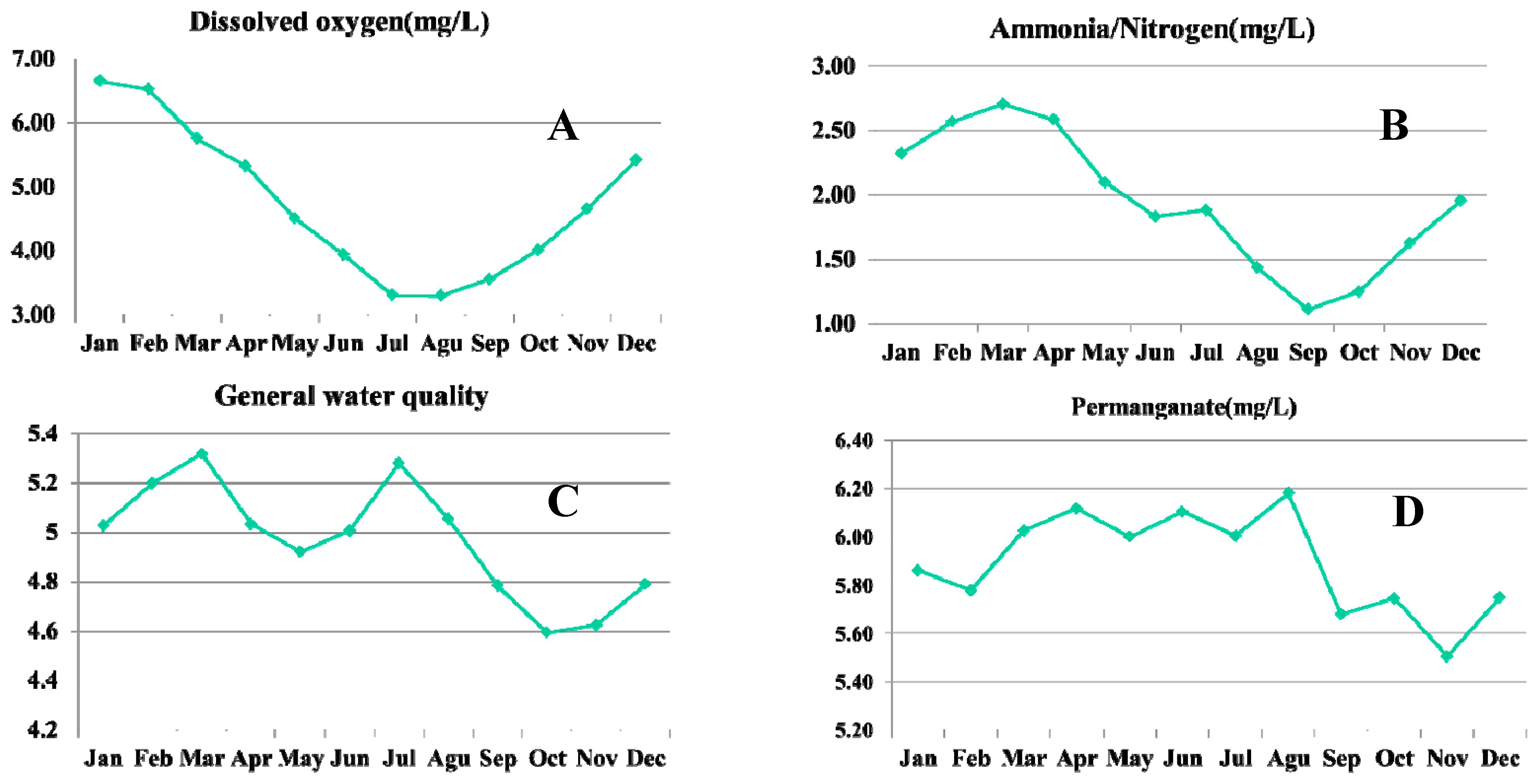
3.3. Water Quality Patterns and Urbanization Impacts

A total of 10 correlation analyses were conducted in this study between the 8640 data records of the five water indicators (i.e., total wastewater, GWQ, DO, ammonia nitrogen, and Permanganate index) with IURB for 2007 and 2015, respectively. All correlations were significant at a confidence level of 0.05, except for GWQ and the permanganate index in 2007. The total wastewater volume in both years was not significantly related to the IURB and, therefore, was not included in this study. The Pearson’s r values ranged from 0.26 to 0.53. Though we tried to recognize the general spatial variance of urbanization processes among the unit watersheds and the local differences within the unit watersheds by giving the weight for each LULC type at the pixel level, the correlation analysis results can be affected by human error introduced during the classification process. Figure 4 displays the scatterplots (a total of six) with significant relationships in each year. Results showed that higher IURB values (namely, a greater urban area) were associated with a decrease in DO, an increase in ammonia nitrogen and the permanganate index and, in general, poor water quality. Similar patterns were identified in 2007 and 2015 with the same indicators: DO and ammonia nitrogen. Also, the absolute values of DO (higher) and ammonia nitrogen (lower) in 2015 showed that there was better water quality compared to 2007.
Seasonal variations of the four water quality indicators in Table 4 were analyzed from January to December (monthly records averaged) in each year from 2007 to 2015. Results showed quite strong seasonal trends throughout the research period (Figure 5). Specifically, the DO concentrations in water decreased with increasing temperature, as confirmed by the lowest DO concentrations in July and August (Figure 5A). DO is considered the most crucial factor to water quality and aquatic organisms [43] and, therefore, is a crucial condition for fisheries. DO values ranging between 4 to 15 mg/L is ideal for surface water fish. Abnormally low or high DO concentrations result in fish mortality or gas bubble disease [44,45]. One peak (in March) and one trough (in September) were found in the ammonia nitrogen seasonal trend (Figure 5B). This pattern can be explained by the agricultural activity and urbanization process in Shanghai. The profile of ammonia nitrogen did not follow the exact conclusion from Xie et al.’s study that the level of ammonia nitrogen is lowest during the winter season [41]. However, ammonia nitrogen can be introduced into water systems through animal feces, sewage waste, fossil fuel consumption, and (especially) fertilizers [41,46]. Large amounts of fossil fuel are burnt during the winter seasons (December, January, and February) in urban area of Shanghai. The emissions enter the water system through precipitation in spring. Nitrogen is an important nutrient and it consumes oxygen in water bodies [41,47].
Two peaks and two troughs were identified from the GWQ trajectory (Figure 5C). The first peak emerged in March when the agricultural practices started; the second peak arose in July, with the extensive usage of water by citizens during the hottest time of the year. Permanganate (i.e., the permanganate index) is commonly used as an oxidant for controlling the taste of water and clarifying water bodies [48]. It is usually measured through chemical oxygen demand (COD) and applied as an evaluation of water pollution from organic and inorganic oxide materials. It showed a more complex trend in Figure 5D. From March to August, the permanganate index remained at a consistently high level throughout the year, although it was relatively lower between September and February. The permanganate index is a vital indicator for sewage and surface water quality [48]. The months of March to August are relatively warm in Shanghai, and more frequent anthropogenic activities intensified the permanganate index level. Water temperatures also influence permanganate index concentrations in water systems.
Using the regression models established in Figure 5, the simulated distributions of the four water quality indicators in 2015 are mapped in Figure 6. The GWQ (Figure 6A), permanganate (Figure 6B), and ammonia nitrogen (Figure 6C) levels showed similar spatial patterns while that of DO was the opposite (Figure 6D). In general, water quality is lower in the urbanized area, especially in the CBDs. The Jinshan and Chongming areas maintain a relatively better water quality. Poor water quality can suppress the dissolved oxygen content. Thus, a large amount of permanganate is often applied to treat water. Urban sewage can carry a considerable volume of ammonia nitrogen.
Temporal changes of water quality were extracted to further investigate the relationships between water quality and the urbanization processes in Shanghai. Only DO and ammonia nitrogen were compared between 2007 and 2015 because they were significantly related to urban index in both years (Figure 7), while the GWQ and permanganate index were not significant in 2007 (Table 4). In Kannel et al.’s research [49], DO by itself showed very promising applications in explaining water quality classification (93%) compared to a more complex water quality index (90% for the combination of temperature, DO, pH, electrical conductivity, and total suspended solids). The official records have shown that the overall water quality in Shanghai was slightly improved from 2007 to 2015, which may be attributed to strict environmental regulations from the government after the 2010 Shanghai EXPO [50]. In our study, two major clusters (one improving and the other degrading) were identified in both maps (Figure 7A,B). DO and ammonia nitrogen showed the opposite trend around the same areas. When combining the urbanization map (also shown in Figure 3B), new towns (i.e., Xinchengzhen) emerged in the southeast area of Shanghai from 2007 to 2015, and the local water quality degraded (i.e., DO decreased and ammonia nitrogen increased) in these areas. Water degradation was not recognized (in grey) in other areas of Shanghai, even where urbanization was recognized (in red). Results indicated improvement in the water quality around the north central area (i.e., CBDs and other well developed urban areas), where no new urban areas emerged. With respect to the EXPO event hosted in this region (Xuhui, Pudong, Hongkou districts, etc. located along the Huangpu River), the environment was significantly enhanced with urban greening policies and the Clean Water Act. As mentioned in Yin et al.’s discussion, more wastewater treatment plants would be continuously installed in Shanghai until 2020 [7]. Li et al. demonstrated the successful performance of a two-year water quality treatment applied in central areas of Shanghai, especially with regards to DO and ammonia nitrogen content [51]. Seasonal (Figure 5) and trend (Figure 8) analysis were performed for every station and then overall spatial patterns from observed records, monthly average, and annual average data were displayed. After analyzing all water records from every station during the study period, we also overlaid the cluster maps with water quality monitor stations on the administrative division map (Figure 8). Green dashed lines indicate the severely polluted surface water content level, according to China environmental quality standards (Table 1). Three districts—the central area (Hongkou, Jingan, Xuhui, etc.), Qingpu, and Songjiang—showed an increasing trend of water quality with regards to DO (i.e., slightly increasing) and ammonia nitrogen (i.e., decreasing) values. This pattern matches the low/no urban development and adequate water quality management during the study period [30]. Meanwhile, stations within the Pudong New Area showed the degradation of water quality (ammonia nitrogen, particularly) alongside the urbanization process. The Yanhshupu and Qixian stations were displayed as examples. The spatial pattern and temporal trend consistent with findings in Yin et al.’s (2000), Ren et al.’s (1947–1996), and Wang et al.’s (1982–2005) studies [7,10,30]. Urbanization accelerates the degradation of water quality, while strict environmental management has effectively inhibited the deterioration of water quality, even improving it [7,10,29,30,51].

4. Conclusions

This study employed a water quality regression model based on sampled water quality variables and the satellite-extracted urban land use change of Shanghai, China from 2007 to 2015. This model was used to explore the impacts of urbanization on the water quality of this megacity. The results revealed that water quality was affected by the urbanization process and water use policy. Degraded water quality was observed in suburban outskirts due to intensified land development. Improved water quality can be credited to the enforced wastewater discharge regulations in the CBDs of Shanghai, for example, during a global event (EXPO) in this study period. Water quality changes with urbanization processes are mapped across the study area, and poor water quality areas deserve higher attention from local authorities. The trajectory of city development is always surprisingly similar: compromising the environment for more significant economic growth. Shanghai is no exception. The local authority from the Pudong New Area should learn from the central areas about water quality management. This study indicates that, while the point collection of pollution data is usually incapable of comprehensive water quality analysis, its integration with satellite imagery improves the spatial representations across a large city at a watershed level. Though urbanization processes could be represented by population density, GDP, build-up surface, etc., previous literature have demonstrated the issues of using these representors [31]. Five water indicators were applied considering the sensitivity and limited accessibility of water quality data. Given the convenience of using RS and GIS to preform to real-time monitoring LULC changes, with its higher resolution of satellite images, there could be an increase in the accuracy and feasibility of applying the methods in the study to water quality management and an improvement in the immediate response to abnormal environmental changes. For the future, the SWAT model can be adopted if more data is available. This study contributes to the literature of water quality in urban environments from a spatial perspective. While urbanization is accelerating globally, approaches developed in this study could be applied to investigate long-term urbanization effects on water quality at various spatial scales. When a more detailed wastewater data set becomes available, waterborne disease data could be further examined to investigate the health outcomes of urbanization with water quality degradation.

Author Contributions

H.L. designed the analytical framework of this study and drafted the manuscript. C.W. provided methodological advice and made major revisions of the manuscript. X.H. and H.L. conducted GIS and statistical analysis. A.H. assisted in collecting and processing data and provided both GIS and RS analysis.

Funding

This research received no external funding.

Acknowledgments

The authors would like to thank Allan James, Yuqin Jiang the anonymous reviewers, and the guest editor for their constructive comments and suggestions, which greatly improved the quality of the manuscript.

Conflicts of Interest

The authors declare no conflict of interest.

References

  1. World Resource Institute. 2007. Available online: http://www.wri.org/publication/wri-annualreport-2006–2007 (accessed on 21 April 2015).
  2. Bao, L.J.; Maruya, K.A.; Snyder, S.A.; Zeng, E.Y. China’s water pollution by persistent organic pollutants. Environ. Pollut. 2012, 163, 100–108. [Google Scholar] [CrossRef] [PubMed]
  3. Li, H.; Li, Y.; Lee, M.K.; Liu, Z.; Miao, C. Spatiotemporal analysis of heavy metal water pollution in transitional China. Sustainability 2015, 7, 9067–9087. [Google Scholar] [CrossRef]
  4. Li, Y.; Li, H.; Liu, Z.; Miao, C. Spatial Assessment of Cancer Incidences and the Risks of Industrial Wastewater Emission in China. Sustainability 2016, 8, 480. [Google Scholar] [CrossRef]
  5. Zhang, R.; Hamerlinck, J.D.; Gloss, S.P.; Munn, L. Determination of Nonpoint-Source Pollution Using GIS and Numerical Models. J. Environ. Qual. 1996, 25, 411–418. [Google Scholar] [CrossRef] [Green Version]
  6. Ebenstein, A. The consequences of industrialization: Envidence from water pollution and digestive cancers in China. Rev. Econ. Stat. 2012, 94, 186–201. [Google Scholar] [CrossRef]
  7. Yin, Z.Y.; Walcott, S.; Kaplan, B.; Cao, J.; Lin, W.; Chen, M.; Liu, D.; Ning, Y. An analysis of the relationship between spatial patterns of water quality and urban development in Shanghai, China. Comput. Environ. Urban Syst. 2005, 29, 197–221. [Google Scholar] [CrossRef]
  8. Zhao, S.; Da, L.; Tang, Z.; Fang, H.; Song, K.; Fang, J. Ecological consequences of rapid urban expansion: Shanghai, China. Front. Ecol. Environ. 2006, 4, 341–346. [Google Scholar] [CrossRef] [Green Version]
  9. Zhang, H. The orientation of water quality variation from the metropolis river–Huangpu River, Shanghai. Environ. Monit. Assess. 2007, 127, 429–434. [Google Scholar] [CrossRef] [PubMed]
  10. Wang, J.; Da, L.; Song, K.; Li, B.L. Temporal variations of surface water quality in urban, suburban and rural areas during rapid urbanization in Shanghai, China. Environ. Pollut. 2008, 152, 387–393. [Google Scholar] [CrossRef] [PubMed]
  11. Jiang, L.; Hu, X.; Yin, D.; Zhang, H.; Yu, Z. Occurrence, distribution and seasonal variation of antibiotics in the Huangpu River, Shanghai, China. Chemosphere 2011, 82, 822–828. [Google Scholar] [CrossRef] [PubMed]
  12. Jiang, L.; Hu, X.; Xu, T.; Zhang, H.; Sheng, D.; Yin, D. Prevalence of antibiotic resistance genes and their relationship with antibiotics in the Huangpu River and the drinking water sources, Shanghai, China. Sci. Total Environ. 2013, 458, 267–272. [Google Scholar] [CrossRef] [PubMed]
  13. China Statistical Yearbook, Shanghai, China. The Central People’s Government of the People’s Republic of China, The People’s Republic of China Yearbook. 2015. Available online: http://www.gov.cn/test/2005-07/27/content_17403.htm (accessed on 13 July 2015).
  14. Li, H.; Wang, C.; Jiang, Y.; Hug, A.; Li, Y. Spatial assessment of sewage discharge with urbanization in 2004–2014, Beijing, China. AIMS Environ. Sci. 2016, 3, 842–857. [Google Scholar] [CrossRef]
  15. Coskun, H.G.; Gulergun, O.; Yilmaz, L. Monitoring of protected bands of Terkos drinking water reservoir of metropolitan Istanbul near the Black Sea coast using satellite data. Int. J. Appl. Earth Obs. Geoinf. 2006, 8, 49–60. [Google Scholar] [CrossRef]
  16. Asadi, S.S.; Vuppala, P.; Anji Reddy, M. Remote Sensing and GIS Techniques for Evalution of Groundwater Quality in Municipal Corporation of Hyderabad (Zone-V), India. Int. J. Environ. Res. Public Health 2007, 4, 45–52. [Google Scholar] [CrossRef] [PubMed]
  17. Satapathy, D.R.; Salve, P.R.; Katpatal, Y.B. Spatial distribution of metals in ground/surface waters in the Chandrapur district (Central India) and their plausible sources. Environ. Geol. 2009, 56, 1323–1352. [Google Scholar] [CrossRef]
  18. Dede, O.T.; Telci, I.T.; Aral, M.M. The use of water quality index models for the evaluation of surface water quality: A case study for Kirmir Basin, Ankara, Turkey. Water Qual. Expos. Health 2013, 5, 41–56. [Google Scholar]
  19. Wang, M.; Webber, M.; Finlayson, B.; Barnett, J. Rural industries and water pollution in China. J. Environ. Manag. 2008, 86, 648–659. [Google Scholar] [CrossRef] [PubMed]
  20. Foster, J.A.; McDonald, A.T. Assessing pollution risks to water supply intakes using geographical information systems (GIS). Environ. Model. Softw. 2000, 15, 225–234. [Google Scholar] [CrossRef]
  21. Yang, T.; Liu, J. Health Risk Assessment and Spatial Distribution Characteristic on Heavy Metals Pollution of Haihe River Basin. J. Environ. Anal. Toxicol. 2012, 2, 152. [Google Scholar] [CrossRef]
  22. Wang, Y.; Wang, P.; Bai, Y.; Tian, Z.; Li, J.; Shao, X.; Mustavich, L.F.; Li, B.L. Assessment of surface water quality via multivariate statistical techniques: A case study of the Songhua River Harbin region, China. J. Hydro-Environ. Res. 2013, 7, 30–40. [Google Scholar] [CrossRef]
  23. Soil and Water Assessment Tool (SWAT). 2012. Available online: http://swat.tamu.edu/ (accessed on 27 June 2016).
  24. Zhang, J.; Mauzerall, D.; Zhu, T.; Liang, S.; Ezzati, M.; Remais, J.V. Environmental health in China: Progress towards clean air and safe water. Lancet 2010, 375, 1110–1119. [Google Scholar] [CrossRef]
  25. Liu, Q.; Xie, W.; Xia, J. Using Semivariogram and Moran’s I Techniques to Evaluate Spatial Distribution of Soil Micronutrients. Commun. Soil Sci. Plant Anal. 2013, 44, 1182–1192. [Google Scholar] [CrossRef]
  26. Lee, C.C.; Chiu, Y.B.; Sun, C.H. The environmental Kuznets curve hypothesis for water pollution: Do regions matter? Energy Policy 2010, 38, 12–23. [Google Scholar] [CrossRef]
  27. Liu, J.; Zhang, X.; Tran, H.; Wang, D.Q.; Zhu, Y.N. Heavy metal contamination and risk assessment in water, paddy soil, and rice around an electroplating plant. Environ. Sci. Pollut. Res. 2011, 18, 1623–1632. [Google Scholar] [CrossRef] [PubMed]
  28. Schwarzenbach, R.P.; Egli, T.; Hofstetter, T.B.; Von Gunten, U.; Wehrli, B. Global water pollution and human health. Annu. Rev. Environ. Resour. 2010, 35, 109–136. [Google Scholar] [CrossRef]
  29. He, H.; Zhou, J.; Wu, Y.; Zhang, W.; Xie, X. Modelling the response of surface water quality to the urbanization in Xi’an, China. J. Environ. Manag. 2008, 86, 731–749. [Google Scholar] [CrossRef] [PubMed]
  30. Ren, W.; Zhong, Y.; Meligrana, J.; Anderson, B.; Watt, W.E.; Chen, J.; Leung, H.L. Urbanization, land use, and water quality in Shanghai: 1947–1996. Environ. Int. 2003, 29, 649–659. [Google Scholar] [CrossRef]
  31. Wu, S.S.; Qiu, X.; Wang, L. Population estimation methods in GIS and remote sensing: A review. GIScience Remote Sens. 2005, 42, 80–96. [Google Scholar] [CrossRef]
  32. Cui, L.; Shi, J. Urbanization and its environmental effects in Shanghai, China. Urban Clim. 2012, 2, 1–15. [Google Scholar] [CrossRef]
  33. Li, J.J.; Wang, X.R.; Wang, X.J.; Ma, W.C.; Zhang, H. Remote sensing evaluation of urban heat island and its spatial pattern of the Shanghai metropolitan area, China. Ecol. Complex. 2009, 6, 413–420. [Google Scholar] [CrossRef]
  34. Chen, S.; Zeng, S.; Xie, C. Remote sensing and GIS for urban growth analysis in China. Photogramm. Eng. Remote Sens. 2000, 66, 593–598. [Google Scholar]
  35. Wei, C.; Taubenböck, H.; Blaschke, T. Measuring urban agglomeration using a city-scale dasymetric population map: A study in the Pearl River Delta, China. Habitat Int. 2017, 59, 32–43. [Google Scholar] [CrossRef]
  36. Alexander, R.B.; Boyer, E.W.; Smith, R.A.; Schwarz, G.E.; Moore, R.B. The role of headwater streams in downstream water quality. JAWRA J. Am. Water Resour. Assoc. 2007, 43, 41–59. [Google Scholar] [CrossRef] [PubMed]
  37. United States Geological Survey. 2008. Available online: http://earthexplorer.usgs.gov/ (accessed on 13 July 2015).
  38. China Data Center. 2015. Available online: https://chinadatacenter.org/ (accessed on 27 January 2015).
  39. Quality Standard for Ground Water. 2002. Available online: http://g2g.tx.gov.cn/art/2015/10/13/art_97_53143.html (accessed on 5 December 2015). (In Chinese).
  40. Zang, C.; Huang, S.; Wu, M.; Du, S.; Scholz, M.; Gao, F.; Lin, C.; Guo, Y.; Dong, Y. Comparison of relationships between pH, dissolved oxygen and chlorophyll a for aquaculture and non-aquaculture waters. Water Air Soil Pollut. 2011, 219, 157–174. [Google Scholar] [CrossRef]
  41. Xie, J.; Liu, H.; Wang, A. The role of ammonia nitrogen, total nitrogen, trinitrogen conversion, and ammonia nitrogen in water pollution assessment and control. Inner Mong. Water Resour. 2011, 5, 34–36. (In Chinese) [Google Scholar]
  42. Li, Z.; Zhong, Z. Analysis of the relationship among BOD, chemical oxygen demand, and permanganate index. Tech. Superv. Water Resour. 2015, 23, 5–6. (In Chinese) [Google Scholar]
  43. Murphy, R.R.; Curriero, F.C.; Ball, W.P. Comparison of spatial interpolation methods for water quality evaluation in the Chesapeake Bay. J. Environ. Eng. 2009, 136, 160–171. [Google Scholar] [CrossRef]
  44. Fundamentals of Environmental Measurements. Available online: http://www.fondriest.com/environmental-measurements/ (accessed on 27 January 2015).
  45. McCutcheon, S.C.; Martin, J.L.; Barnwell, T.O. Water quality. Handb. Hydrol. 1993, 11, 73. [Google Scholar]
  46. Viessman, W.; Hammer, M.J.; Perez, E.M.; Chadik, P. Water Supply and Pollution Control; Pearson Prentice Hall: Upper Saddle River, NJ, USA, 2009. [Google Scholar]
  47. International Organization for Standardization: Water Quality—Determination of Permanganate Index. 1993. Available online: https://www.iso.org/standard/15669.html (accessed on 5 December 2016).
  48. Tucker, C.S.; Boyd, C.E. Relationships between potassium permanganate treatment and water quality. Trans. Am. Fisheries Soc. 1977, 106, 481–488. [Google Scholar] [CrossRef]
  49. Kannel, P.R.; Lee, S.; Lee, Y.S.; Kanel, S.R.; Khan, S.P. Application of water quality indices and dissolved oxygen as indicators for river water classification and urban impact assessment. Environ. Monit. Assess. 2007, 132, 93–110. [Google Scholar] [CrossRef] [PubMed]
  50. Shanghai Environmental Protection Bureau. 2010. Available online: http://www.sepb.gov.cn/fa/cms/upload/uploadFiles/2011-11-09/file675.pdf (accessed on 5 December 2016).
  51. Li, X.; Manman, C.; Anderson, B.C. Design and performance of a water quality treatment wetland in a public park in Shanghai, China. Ecol. Eng. 2009, 35, 18–24. [Google Scholar] [CrossRef]
Figure 1. An example Landsat 8 OLI image (SWIR/NIR/R composition) of the study area. Water sample points and unit watersheds are overlaid in the image.
Remotesensing 10 01024 g001
Figure 2. (A) Classification results of Shanghai (2007). (B) Urban expansion in Shanghai between 2007 and 2015.
Remotesensing 10 01024 g002
Figure 3. The IURB and its changes between 2007 and 2015. (A) The 2015 Urban Index (IURB). (B) The 2007–2015 Urban Index Change.
Remotesensing 10 01024 g003
Figure 4. Relationships between water quality indicators and IURB.
Remotesensing 10 01024 g004aRemotesensing 10 01024 g004b
Figure 5. Seasonal changes of water quality indicators: (A) DO, (B) ammonia nitrogen, (C) GWQ, and (D) permanganate index.
Remotesensing 10 01024 g005
Figure 6. Spatial distributions of the four modeled water quality indicators in 2015: (A) GWQ; (B) permanganate; (C) ammonia nitrogen; and (D) DO.
Remotesensing 10 01024 g006
Figure 7. Water quality changes with urbanization from 2007 to 2015: (A) ammonia nitrogen changes and (B) DO changes.
Remotesensing 10 01024 g007
Figure 8. Water quality changes in stations from 2007 to 2015: (A) ammonia nitrogen changes and (B) DO changes. Note: Green dashed lines indicate the severely polluted surface water content level, according to China environmental quality standards.
Remotesensing 10 01024 g008
Table 1. China Environmental quality standards for ground water (GB3838-2002).
Water Quality ExcellentGoodSlightly PollutedPollutedSeverely Polluted
General Water Quality Class IIIIIIIVV
Dissolved OxygenSaturation rate 90% or 7.56532
Permanganate Index2461015
Ammonia Nitrogen0.150.51.01.52.0
Table 2. Accuracy assessment for the classification of the 2007 image.
ClassTruth PointsProducer AccuracyOmission ErrorUser’s AccuracyCommission ErrorConditional Kappa
Water13100%0%100%0%1
Forest59100%0%85%15%0.81
Bare soil2893%7%100%0%1
Agricultural land5186%14%100%0%1
Low urban1781%19%100%0%1
Medium urban62100%0%92%8%0.90
High urban20100%0%100%0%1
Overall Accuracy94.40%
Overall Kappa0.93
Table 3. Accuracy assessment for the classification of the 2015 image.
ClassTruth PointsProducer AccuracyOmission ErrorUser’s AccuracyCommission ErrorConditional Kappa
Water21100%0%100%0%1
Forest 7497%3%89%11%0.85
Bare soil17100%0%88%12%0.87
Agricultural land3880%20%97%3%0.97
Low urban2481%19%88%12%0.86
Medium urban4896%4%98%2%0.97
High urban2896%4%86%14%0.84
Overall Accuracy92.4%
Overall Kappa0.91
Table 4. Correlation coefficients (Pearson’s r) of IURB and water quality data.
General Water QualityDissolved OxygenAmmonia NitrogenPermanganate Index
2007 UI0.27−0.66 ** 0.67 ** 0.03
0.44 0.45
2015 UI0.67 ** −0.68 ** 0.51 ** 0.72 **
0.45 0.46 0.53 0.26
Note: ** indicates p < 0.05.

