Estimation of AOD Under Uncertainty: An Approach for Hyperspectral Airborne Data

Abstract

A key parameter for atmospheric correction (AC) is Aerosol Optical Depth (AOD), which is often estimated from sensor radiance ($L_{\mathrm{rs},\mathrm{t}}\left(\lambda \right)$). Noise, the dependency on surface type, viewing and illumination geometry cause uncertainty in AOD inference. We propose a method that determines pre-estimates of surface reflectance (${\rho }_{\mathrm{t},\mathrm{pre}}$) where effects associated with $L_{\mathrm{rs},\mathrm{t}}\left(\lambda \right)$ are less influential. The method identifies pixels comprising pure materials from ${\rho }_{\mathrm{t},\mathrm{pre}}$. AOD values at the pure pixels are iteratively estimated using $l_2$-norm optimization. Using the adjacency range function, the AOD is estimated at each pixel. We applied the method on Hyperspectral Mapper and Airborne Prism Experiment instruments for experiments on synthetic data and on real data. To simulate real imaging conditions, noise was added to the data. The estimation error of the AOD is minimized to 0.06–0.08 with a signal-to-reconstruction-error equal to 35 dB. We compared the proposed method with a dense dark vegetation (DDV)-based state-of-the-art method. This reference method, resulted in a larger variability in AOD estimates resulting in low signal-to-reconstruction-error between 5–10 dB. For per-pixel estimation of AOD, the performance of the reference method further degraded. We conclude that the proposed method is more precise than the DDV methods and can be extended to other AC parameters.

1. Introduction

Hyperspectral imaging sensors record the at-sensor radiance reflected from a surface, for hundreds of narrow contiguous spectral bands. The wealth of spectral information available from advanced hyperspectral imaging instruments has opened new perspectives in many application domains. For example, monitoring of natural grasslands and the synanthropic patterns of invasive species [1], mapping of tree species in a complex mixed forest ecosystem [2] and analyzing the dominant minerals and rocks in a mountain region [3], mapping and estimation of the amounts of hazardous materials to human health [4] and urban land-cover mapping with high resolution images [5] are among others. Besides, retrieving the atmospheric condition parameters aid to the atmospheric correction and the atmosphere monitoring processes. For instance, estimation of aerosol optical depth [6] and estimation column water vapor [7], and the monitoring of nitrogen dioxide (NO${}_2$) [8] using the hyperspectral data.

A pixel of a three dimensional datacube recorded by a hyperspectral sensor comprises radiation measured by the sensor, at hundreds of wavelengths. In the absence of the Earth’s atmosphere, a reflectance obtained from the recorded radiation is the spectral signature that characterises the underlying surface within the Instantaneous Field of View of the sensor. In the presence of the Earth’s atmosphere, however, the apparent reflectance differs from the target reflectance. This is primarily because of the complex interaction of the surface reflected radiation with the atmospheric constituents while propagating along the path from the target surface to the sensor. The interaction generates two main atmospheric effects: absorption by atmospheric gases (in particular water vapour and ozone) and aerosols (in the visible and near infrared spectral range) and scattering by aerosols and larger atmospheric gas molecules. In addition, on the path of beam to the sensor two major scattering components distort the at sensor radiance: reflection by the surrounding area of the target pixel and the radiance backscattered by the atmosphere.

An Atmospheric Correction (AC) algorithm is commonly applied to retrieve the radiance reflected at the surface from the at-sensor radiance. AC algorithms can be classified into scene-based empirical algorithms and algorithms based on radiative transfer modeling. As radiative transfer modeling is mature for routine processing of hyperspectral image data, we will use its algorithms in this article [9]. Over the years, a range of radiative transfer-based atmospheric correction methods have been developed for hyperspectral data. Some of these methods include Atmosphere REMoval (ATREM), High Accuracy ATmospheric Correction for Hyperspectral data (HATCH), Imaging Spectrometer Data Analysis System (ISDAS), Atmospheric CORrection Now (ACORN), Fast Line-of-sight Atmospheric Analysis of Spectral Hypercubes (FLAASH) and ATmospheric CORection (ATCOR). A comprehensive review is given in [10].

This article specifically focuses on an operational processing chain. An operational processing chain is implemented in the multi-mission Processing, Archiving, and distribution Facility (PAF) for Earth observation products [11]. Experiments in this article are performed using the Central Data Processing Center (CDPC), a PAF at the Flemish Institute for Technological Research (VITO, Belgium) [12]. In the CDPC, the MODTRAN interrogation technique-based atmospheric correction converts the at-sensor radiance to Hemispherical-Directional Reflectance Factor (HDRF) values for land targets. As a part of the overall atmospheric correction process additional supporting algorithms are included to account for correcting for adjacency effect, haze and shadow correction, topographic BRDF correction. Following these corrections, some of the supporting modules used in the CDPC are: (a) orthorectification module for a full characterization of viewing and illumination geometry; (b) wavelength shift detection module, applied to the data prior to the atmospheric correction process; (c) spectral resampling module, to account for the smile effects, i.e., the central wavelength depends slightly on the column pixel location; and (d) spectral smoothing module, to remove some spectral artifacts, a wavelength dependent spectral smoothing of the data might be required. Additionally, correction for adjacency effects, and use of topographic and kernel BRDF corrections can be employed [13].

In radiative transfer modeling, the target reflected radiance can be derived assuming a plane parallel geometry of the atmosphere, whereas the viewing and illumination geometry are known while some inference of the total optical depth of the atmosphere is required. For this inference, the concentration of the atmospheric scatterers and absorbers should be available at the time of imaging. Both absorbers, water vapour, and scatterer, aerosols and gas molecules, are highly varying in space and time. Thus, they are often estimated directly from satellite or airborne (remote) observations.

There is relatively a long history of the quantitative estimation of aerosol optical depth (AOD) from remotely sensed imagery. For example, the works of [14,15] that use multiangular information, the work of [16] that uses polarization information, the works of [17,18,19] that use multispectral information and the works of [20,21] use multitemporal information. Whereas the MODIS science team [17,22,23] has developed the dense dark object method to estimate AOD from MODIS imagery over land surface for climate study. Despite substantial research efforts, pixelwise estimation of AOD is still a challenge within processing and archiving facilities. Most estimation methods use at-sensor radiance where inference of AOD is affected by retrieval uncertainties of the observed surface, atmospheric parameters, and instrumental errors. Additional processing to mitigate those errors are required to have a reliable reflectance product [24]. For instance, the use of reference pixels and averaging the data, say over 10 × 10 pixels, to reduce the influence of noise, requires a significantly larger data volume for analysis. In addition, the uncertainty induced by such processing is often ignored or impossible to model. Further, those estimation methods rely on some surface characteristics. For instance, the dense dark vegetation (DDV) method to estimate AOD that is further developed in [25] is limited to pixels with dense vegetation. For scenes with DDV pixels that are clustered at a few locations, pixelwise estimation of AOD is challenging. These effects and limitations cause uncertainty in the estimation of AOD which likely propagates to reflectance estimates.

Uncertainty, acknowledging that the pixelwise true values of AOD are unavailable because of limited cognition and of limited granularity, is an inherent property of AOD estimation and cannot be eliminated completely. With more information about estimated spectra over a scene and its estimation conditions, however, we can minimize the uncertainty about AOD. This article focuses on such minimization and is a continuation to our previous works [7,26,27]. The objective of this article is to develop a method to estimate AOD. The proposed method retrieve AOD from estimates of surface reflectance at pure pixels, covering a single endmember and iteratively compare them with corresponding spectra stored in a library. Besides, the other novelty of the proposed method estimates AOD considering sensitivity of reflectance to AOD estimates resulting in less processing time. This is in contrast to those methods which focus on the estimation accuracy outside its sensitivity regime, such as the method of visibility estimation in [11] which is implemented in Atmospheric and Topographic Correction for Airborne Imagery (ATCOR 4) processing facilities of the German Aerospace Center (DLR).

2. Theoretical Background

2.1. Basic Atmospheric Effect Modeling

The surface reflects a fraction ${\rho }_{\mathrm{t}}$ of the total irradiance at the surface $E_{\mathrm{g}}$. This fraction depends on the type of surface, the sun zenith and azimuth angle ${\theta }_{\mathrm{s}}$ and ${\psi }_{\mathrm{s}}$ respectively, the viewing zenith and azimuth angle ${\theta }_{\mathrm{v}}$ and ${\psi }_{\mathrm{v}}$ respectively and wavelength $\lambda$. On the path of the beam to the sensor other radiation components are added to the radiance reflected by the surface ($L_{\mathrm{t}}\left(\lambda \right)$) due to atmospheric scattering. We distinguish four contributions to the at sensor radiance ($L_{\mathrm{rs},\mathrm{t}}\left(\lambda \right)$):

$$L_{\mathrm{rs},\mathrm{t}}\left(\lambda \right)=L_{\mathrm{t}}\left(\lambda \right)+L_{\mathrm{pa}}\left(\lambda \right)+L_{\mathrm{pb}}\left(\lambda \right)+L_{\mathrm{b}}\left(\lambda \right).$$

(1)

$L_{\mathrm{t}}\left(\lambda \right)$ contains the target surface information, $L_{\mathrm{pa}}\left(\lambda \right)$ and $L_{\mathrm{pb}}\left(\lambda \right)$ are path radiance and background path radiance, respectively, that enter the IFOV of the sensor due to scattering and $L_{\mathrm{b}}\left(\lambda \right)$ is the background radiance, or adjacency effect, being the average radiance of the surrounding surface.

For a target surface with reflectance ${\rho }_{\mathrm{t}}\left(\lambda \right)$ and background reflectance ${\rho }_{\mathrm{bck}}\left(\lambda \right)$, the path radiance, the background path radiance, background radiance, and target radiance are:

$$L_{\mathrm{pa}}\left(\lambda \right)=\frac{1}{\pi }R({\theta }_{\mathrm{v}},{\theta }_{\mathrm{s}},{\psi }_{\mathrm{v}}-{\psi }_{\mathrm{s}})cos\left({\theta }_{\mathrm{s}}\right)F$$

(2)

$$L_{\mathrm{pb}}\left(\lambda \right)=\frac{1}{\pi }{\rho }_{\mathrm{bck}}\left(\lambda \right)T_{\mathrm{diff}}^{+}(\tau ,{\theta }_{\mathrm{v}},\lambda )E_{\mathrm{g}}\left(\lambda \right),$$

(3)

$$L_{\mathrm{b}}\left(\lambda \right)=\frac{1}{\pi }{\rho }_{\mathrm{bck}}\left(\lambda \right)T_{\mathrm{dir}}^{+}(\tau ,{\theta }_{\mathrm{v}},\lambda )E_{\mathrm{g}}\left(\lambda \right),$$

(4)

$$L_{\mathrm{t}}\left(\lambda \right)=\frac{1}{\pi }{\rho }_{\mathrm{t}}\left(\lambda \right)T_{\mathrm{dir}}^{+}(\tau ,{\theta }_{\mathrm{v}},\lambda )E_{\mathrm{g}}\left(\lambda \right),$$

(5)

where the function $R({\theta }_{\mathrm{v}},{\theta }_{\mathrm{s}},{\psi }_{\mathrm{v}}-{\psi }_{\mathrm{s}})$ describes the reflection of light by the atmosphere, $T_{\mathrm{diff}}^{+}$ and $T_{\mathrm{dir}}^{+}$. It expresses upward diffuse and direct transmittances respectively. F is the extraterrestrial solar irradiance [28]. If we define $L_{\mathrm{rs},\mathrm{b}}\left(\lambda \right)$ as:

$$L_{\mathrm{rs},\mathrm{b}}\left(\lambda \right)=L_{\mathrm{pa}}\left(\lambda \right)+L_{\mathrm{pb}}\left(\lambda \right)+L_{\mathrm{b}}\left(\lambda \right),$$

(6)

then the background reflectance can be retrieved as

$${\rho }_{\mathrm{bck}}\left(\lambda \right)=\frac{L_{\mathrm{rs},\mathrm{b}}\left(\lambda \right)-L_{\mathrm{pa}}\left(\lambda \right)}{\left[\frac{1}{\pi }cos\left({\theta }_{\mathrm{s}}\right)T_{\mathrm{tot}}^{+}(\tau ,{\theta }_{\mathrm{v}},\lambda )T_{\mathrm{tot}}^{-}({\theta }_{\mathrm{s}},\lambda )F\right]+S\left[L_{\mathrm{rs},\mathrm{b}}\left(\lambda \right)-L_{\mathrm{pa}}\left(\lambda \right)\right]}.$$

(7)

Here S is the spherical albedo for illumination from below of the atmosphere, $T_{\mathrm{tot}}^{+}(\tau ,{\theta }_{\mathrm{v}},\lambda )$ is the sum of $T_{\mathrm{diff}}^{+}(\tau ,{\theta }_{\mathrm{v}},\lambda )$ and $T_{\mathrm{dir}}^{+}(\tau ,{\theta }_{\mathrm{v}},\lambda )$, likewise $T_{\mathrm{tot}}^{-}$ expresses total downward transmittance from the sun to surface. Substituting the expression for ${\rho }_{\mathrm{bck}}\left(\lambda \right)$, the target reflectance equals

$${\rho }_{\mathrm{t}}\left(\lambda \right)=\frac{L_{\mathrm{rs},\mathrm{t}}\left(\lambda \right)-L_{\mathrm{pa}}\left(\lambda \right)+\left[L_{\mathrm{rs},\mathrm{t}}\left(\lambda \right)-L_{\mathrm{rs},\mathrm{b}}\left(\lambda \right)\right]\frac{T_{\mathrm{dir}}^{+}(\tau ,{\theta }_v,\lambda )}{T_{\mathrm{diff}}^{+}(\tau ,{\theta }_{\mathrm{v}},\lambda )}}{\left[\frac{1}{\pi }cos\left({\theta }_{\mathrm{s}}\right)T_{\mathrm{tot}}^{+}(\tau ,{\theta }_{\mathrm{v}},\lambda )T_{\mathrm{tot}}^{-}({\theta }_{\mathrm{s}},\lambda )F\right]+S\left[L_{\mathrm{rs},\mathrm{b}}\left(\lambda \right)-L_{\mathrm{pa}}\left(\lambda \right)\right]}.$$

(8)

The basic atmospheric effect model is well described in [10,28,29,30,31]. We use MODerate resolution atmospheric TRANsmission version 4.1 (MODTRAN 4) [32] to estimate the radiance components in Equation (8). It represents the computing of absorption and scattering in the terrestrial atmosphere at high spectral resolution [33] and is treated in this thesis as a black box. It allows one to pixelwise solve the DIScrete Ordinate Radiative Transfer (DISORT) [34] for accurate computations of atmospheric multiple scattering. In an operational processing chain, however, the considerable execution time to do so is a problem. Thus, MODTRAN 4 is executed for a uniform Lambertain surface reflectance with a spectrally flat surface albedo of $A_{\mathrm{pp}}=0$, $A_{\mathrm{pp}}=0.5$, and $A_{\mathrm{pp}}=1.0$, to determine the various radiance components for a given atmospheric state and angular geometry. This is called the MODTRAN interrogation technique that has been used in operational processing chains to derive the same radiance component as in Equation (8) [13]. MODTRAN 4 produces four radiance components:

• the total radiance as measured by the sensor, $L_{\mathrm{rs},\mathrm{t}}\left(\lambda \right)$,
• the total path radiance $L_{\mathrm{path}}\left(\lambda \right)$ that consists of the light scattered in the path,
• the total ground radiance that consists of all the light reflected by the surface and traveling directly towards the sensor, $L_{\mathrm{gnd}}\left(\lambda \right)$,
• the direct ground reflectance, $L_{\mathrm{dir}}\left(\lambda \right)$ as a fraction of $L_{\mathrm{gnd}}\left(\lambda \right)$ resulting from direct illumination of the ground surface.

The four components are then linked to various radiance components in Equation (8).

In this research, we assume that ${\rho }_t$ can be obtained at pure pixels using a library of materials known a priori. Assuming that a reverse modeling is performed to estimate initial AOD values. Each estimation of AOD is then fed back to atmospheric correction process, which in turn affect the total upward and downward transmissions to solve Equation (8). The reverse modeling is iteratively performed until the convergence is achieved. Details about the method is given in Section 5.

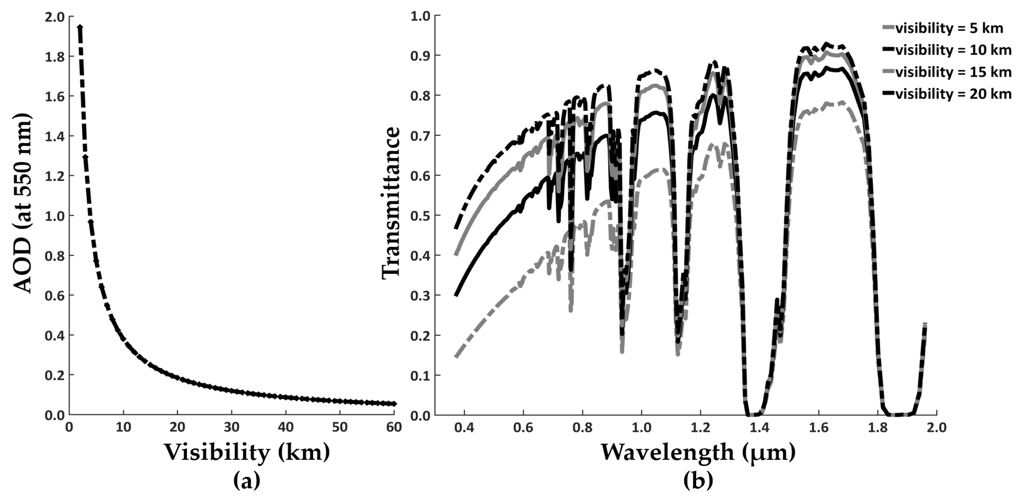
2.2. Aerosol Optical Depth

Aerosols are small particles in suspension in the atmosphere and exist in solid, liquid, and semi-liquid form [35]. Aerosols interact with both solar and terrestrial radiation (the aerosol direct effect) and modify cloud properties (the aerosol indirect effect) [36]. The aerosol particles are characterized by their shape, their size, their chemical composition, and total amount, which in turn determines their radiative characteristics. On regional scale, aerosols characteristics exhibit high variation. For instance, aerosols in urban environments are physically and chemically different from aerosols in remote areas. Further, on local scale, size distribution of urban aerosols varies due to particle growth at high relative humidity and to aerosol interaction with clouds [37]. To accurately quantify aerosol distribution and composition therefore requires continuous observations from sapaceborne instruments, networks of ground-based instruments, and dedicated field experiments.

Sapceborne or airborne remote sensing of aerosol relies on the aerosol optical characteristics i.e., the impact of aerosols on backscattering and transmission of radiation by the Earth’s atmosphere [38]. Thus, with remote sensing aerosol distribution and compositions are not directly quantified. Subsequently, aerosol optical characteristics can be used to obtain total downward and upward transmissions for solving Equation (8). For this purpose, aerosol particles optical properties need to be integrated over the size distribution to obtain the extinction coefficients (${\sigma }_e\left(\lambda \right)$). The aerosol extinction coefficients vary with the location and altitude and their integral over the vertical layer between surface and sensor is called the aerosol optical depth (AOD). AOD is a unitless number, ranging from as low as 0.0 to as high as 3.0. AOD less than 0.1 indicates a low scattering in a clear sky. While AOD greater than 1.0 indicates high scattering in the atmosphere. For airborne remote sensing, values between 0.20 and 0.33 indicates moderate scattering conditions under which most of the airborne capaigns are performed.

The amount of AOD has to be provided into the radiative transfer code as a prior to simulate transmittance due to aerosols. The simulated aerosol transmittance is then used to correct for the influence of aerosols. A popular technique to estimate AOD is to use the sensor recorded radiance $L_{\mathrm{rs},\mathrm{t}}$ on a pixel-by-pixel basis. There is a relatively long history of the quantitative estimation of AOD from $L_{rs,t}$ as discussed in Section 1. Uncertainty arises in the values of AOD because of high variability of aerosols in space and time, lack of continuous observations of aerosols, and limitations of methods to measure AOD from $L_{rs,t}$. We therefore propose a method to iteratively estimate AOD using ${\rho }_t$ instead of $L_{rs,t}$.

3. Datasets

An AOD retrieval algorithm is sensitive to surface albedo [6] and to the scattering conditions [27]. Thus, for exploring the strengths and limitations of the proposed method, spatial configurations and the spectral characteristics of the underlying surface are crucial. For instance, to analyze the scattering of the radiation reflected from dark and bright materials, respectively, a set of scenes comprising pure bright and dark materials are required. Such scenes may exist in nature but remote observation of pure bright or dark targets in a scene through an airborne campaign is quite rare. Thus, we generated five synthetic datasets with physically plausible materials to cover such important cases. Further, synthetic datasets provide an opportunity to experiment under controlled atmospheric conditions such as with low to moderate to high scattering conditions. In addition, we selected a real dataset to test the proposed method under real imaging conditions.

3.1. The Process to Generate the Synthetic Datasets

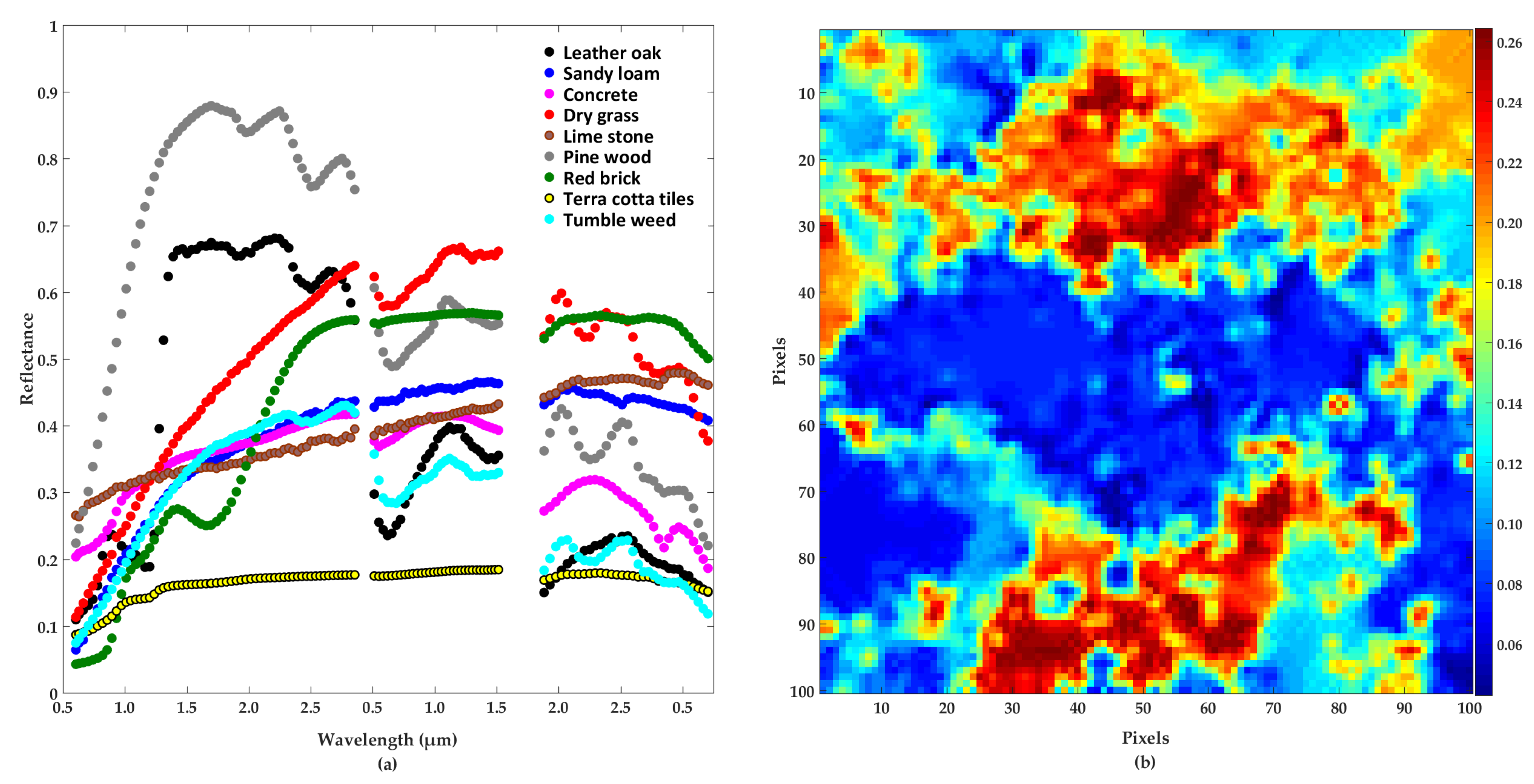
• Spectra of materials are extracted from an existing library. The choice of materials depends on the type of surface required for an experiment. We extract the materials from the database of Jasper Ridge, spectral library [39] available in ENVI software [40] and the database of the Johns Hopkins University Spectral Library [41].
• To generate a sensor specific image, the library is resampled using the sensor response curve. For our experiments, we use response curve of the Hyperspectral Mapper (HyMap) airborne hyperspectral sensor [42].
• Depending on the number of materials, a fraction image comprising abundance of materials is required. We used, MATLAB Hyperspectral Imagery Synthesis tools, available online [43] to generate the abundance images. A convolution of a library of materials with an abundance image generates a synthetic reflectance cube.
• To transform synthetic reflectance to at-sensor radiance, the forward radiative transfer modeling is performed. Details of this modeling are given in Section 4.
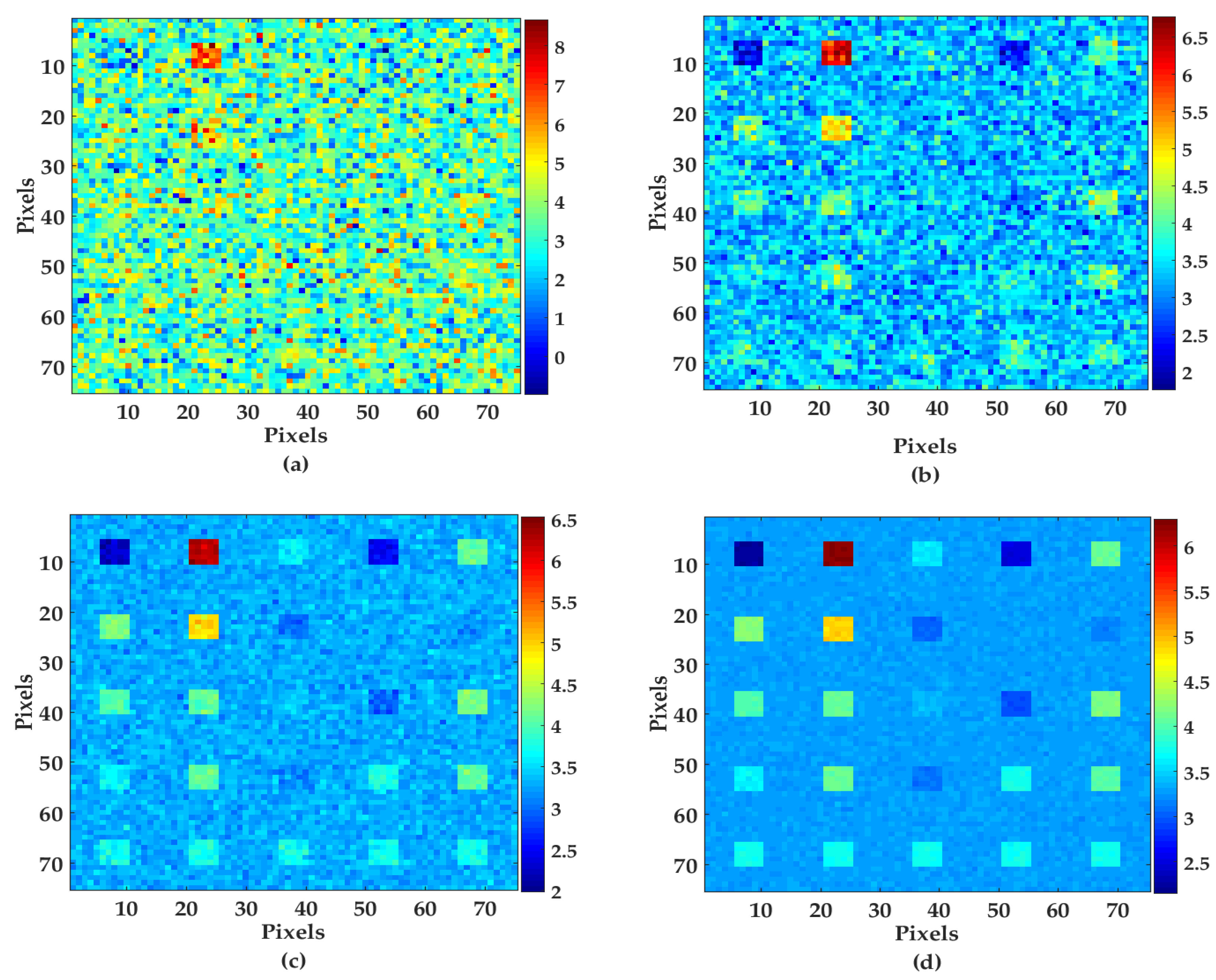
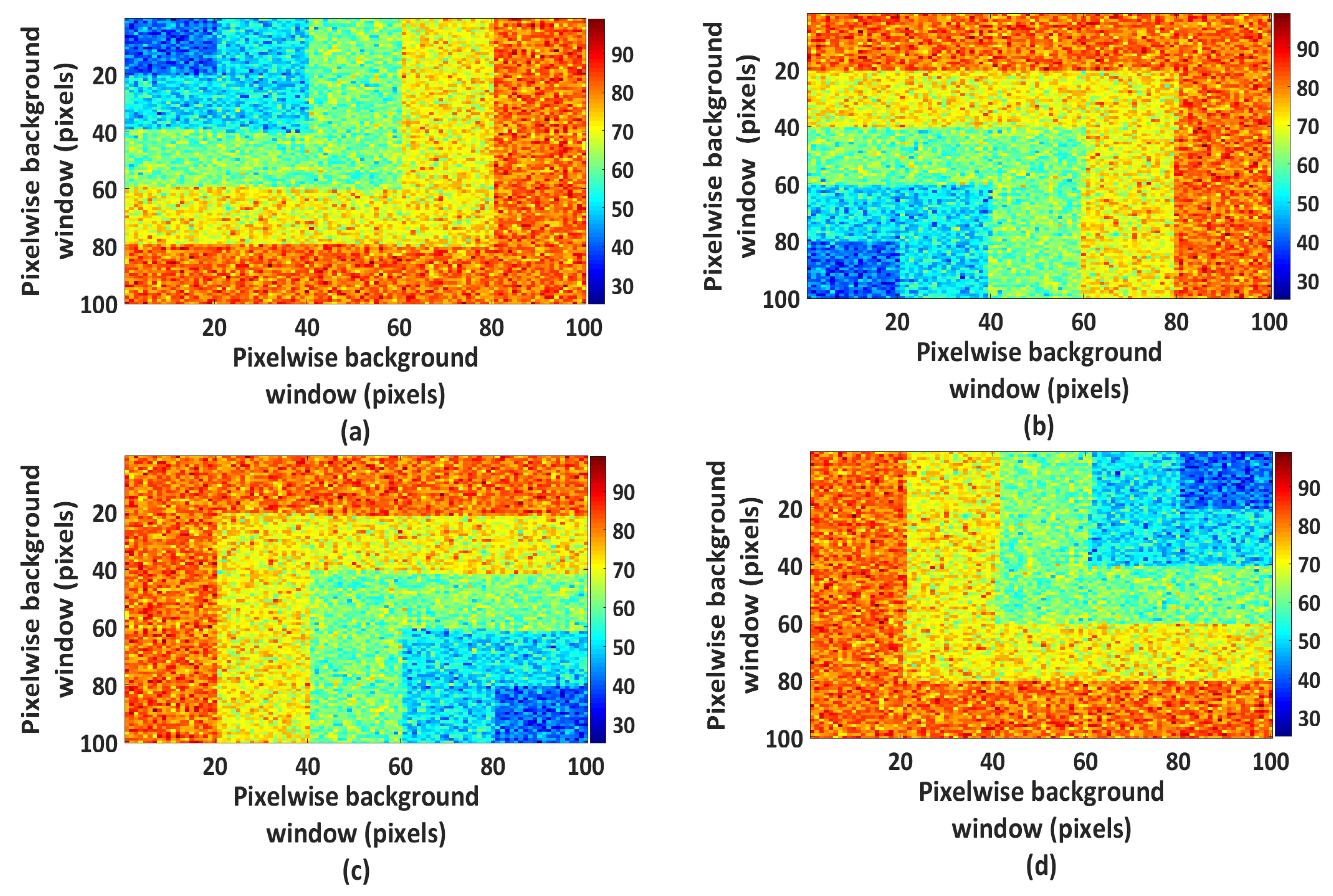
• In a real dataset, sensor noise and processing noise are major sources of distortion. Sensor noise refers to the random electronic noise like dark current, processing noise occurs due to the final pre-processing steps on the reflectance datacube, e.g., spectral smoothing. We added the two types of noise to the datasets at two stages: sensor noise to the radiance cube and processing noise to the estimated reflectance cube. To observe the effect of the different noise levels we considered three levels of the correlated processing noise, with signal-to-noise ratios (SNR):  30, 40, and 50 dB, respectively. All correlated noise levels were generated from independent, normally distributed noise by low-pass filtering with a normalized cut-off frequency of $\frac{8·\pi }{B}$ for each SNR with B being the number of channels. Figure 1 shows four pixelwise estimates of reflectance at 2200 nm (band 100) when SNR of at-sensor radiance was limited to: 30, 40, 50, and 60 dB with random (white) noise. To estimate the four pixelwise reflectance, true AC parameters were employed and no correlated noise was added. When SNR of the at-sensor radiance was limited to 30 dB, 40 dB, and 50 dB the reflectance estimates were severely distorted. Further, [42] suggests that HyMap sensor is highly optimized for mineral exploration tasks which demanded high SNR. From the experiments with the noise levels and following the SNR values given in the literature, we found that sensor noise with SNR = 60 dB was a realistic choice for HyMap sensor.

The size of all the synthetic images is $128\times 128$ pixels with $B=$ 126 spectral bands and the spatial resolution of 2.5 m along track and 2.0 m across track. All synthetic images obey the linear mixture model, which satisfies both the sum to one and the non-negativity constrains and are piecewise smooth, i.e., they are smooth with sharp transitions and exhibit spatial homogeneity, for instance as shown in Figure 2b and Figure 3.

3.2. Case Study: A Vegetation Surface with Usual Scattering Conditions

The objective of using the vegetation surface comprising commonly available materials is to experiment with common airborne imaging conditions. Usual scattering condition refers to moderate scattering conditions with visibility between 23 km to 40 km, approximately equivalent to the AOD range 0.33–0.20. We use spectra of nine materials to generate the image, namely: leather oak, sandy loam, concrete, dry grass, lime stone, pine wood, red brick, terracotta tiles, and tumble weeds. The spectra of the materials and the synthetic vegetation surface are shown in Figure 2 and their fractions in Figure 3.

From visual interpretation of the synthetic vegetation image we found that the spatial variability is spectrally more homogeneous at the center of the image than at the edges and becomes more heterogeneous at the edges (Figure 2b). This is because of the high fraction values of the materials that were present at the edges of the synthetic image (Figure 3). This spatial variability of classes was used as an important criterion to define spatial variability of adjacency range parameter and explained in detail in Section 4.2.

3.3. Case Studies: High Scattering Conditions

The scattering conditions and surface albedo influence the quality of spectra retrieved via atmospheric correction (AC), independently from the other effects. For the proposed method, spectral quality is particularly important for retrieving the pure pixels–a prerequisite of the proposed method–as described in Section 5.2. The following case studies aim to analyze the effect of scattering conditions and surface albedo on the quality of spectra.

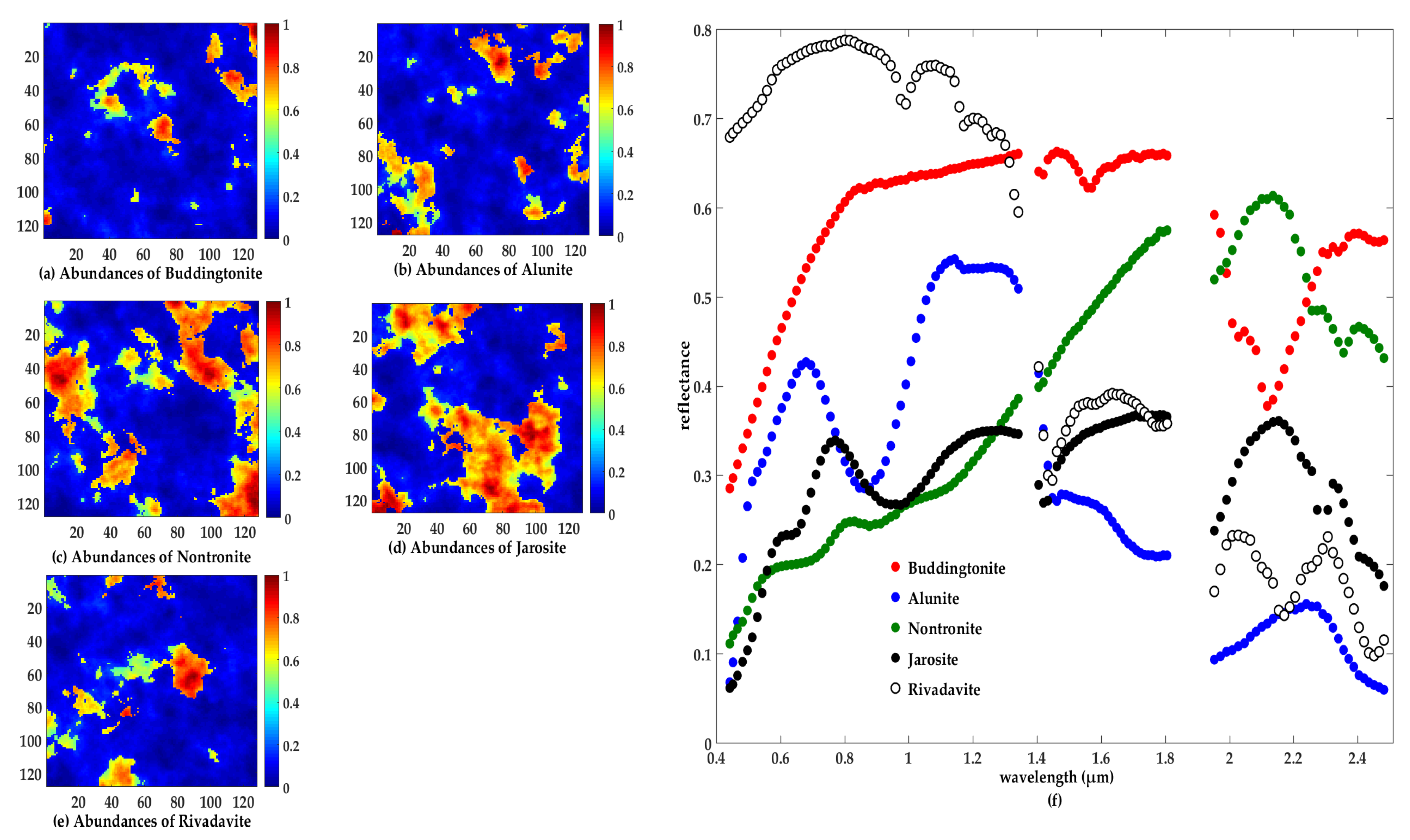
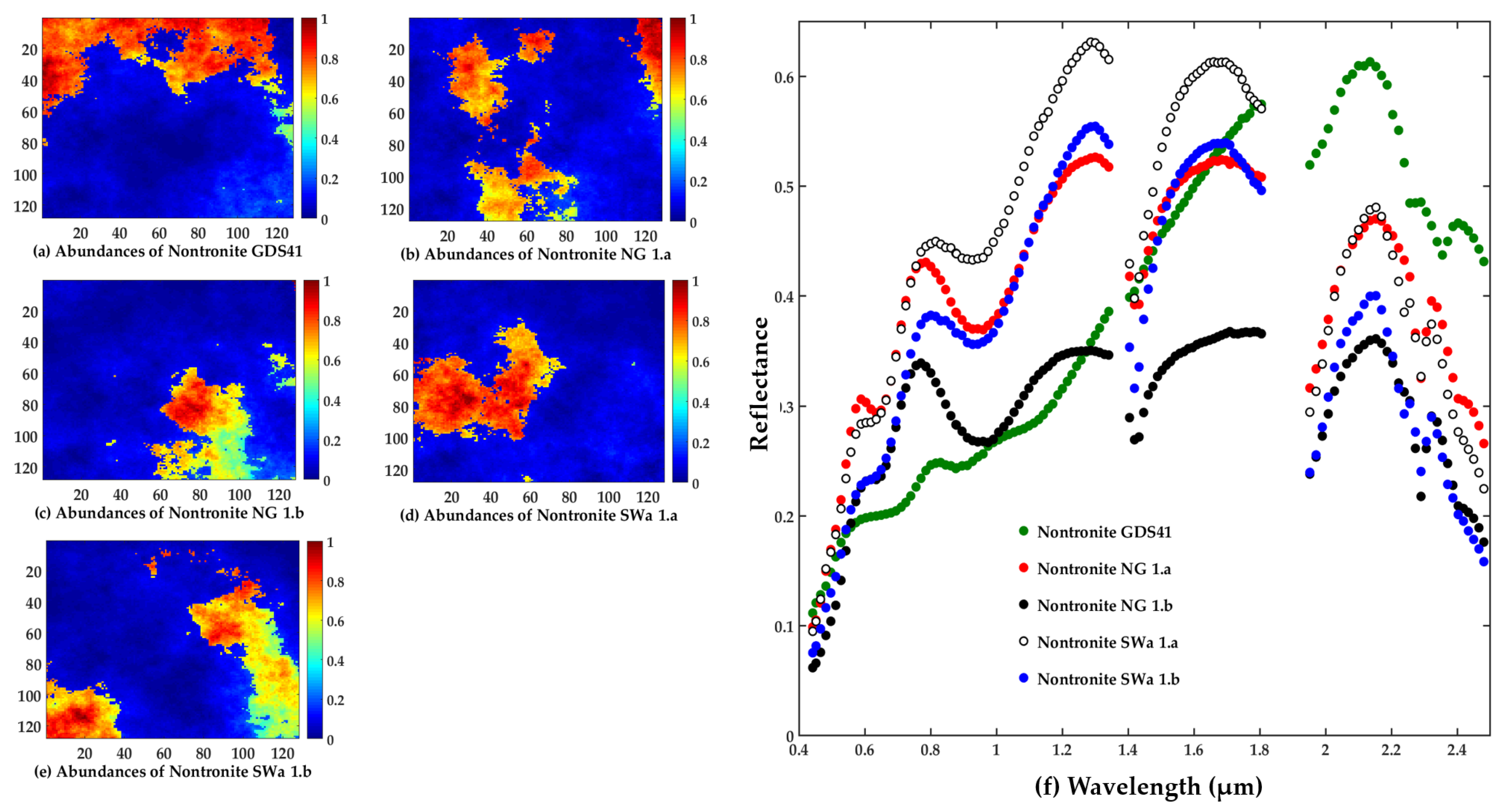
3.3.1. Surfaces with Spectrally Close and Spectrally Distinct Materials

This case study aims to address endmember variability under high scattering conditions using surfaces comprising spectrally distinct and similar materials respectively. Two geological datasets are generated containing two distinct sets of five endmembers, collected from the USGS spectral library [44].

We use the following spectrally distinct endmembers to generate the first geological dataset: Buddingtonite, Alunite, Montmorillonite, Jarosite, and Rivadavite (Figure 4). True fractional abundances of the materials are shown in Figure 4a–e and their spectral profiles are shown in Figure 4f.

The spectrally similar endmembers, used to generate the second geological dataset, were signatures of a single mineral, Nontronite (Figure 5). True fractional abundances of the spectrally similar materials are shown in Figure 5a–e and their spectral profiles are shown in Figure 5f.

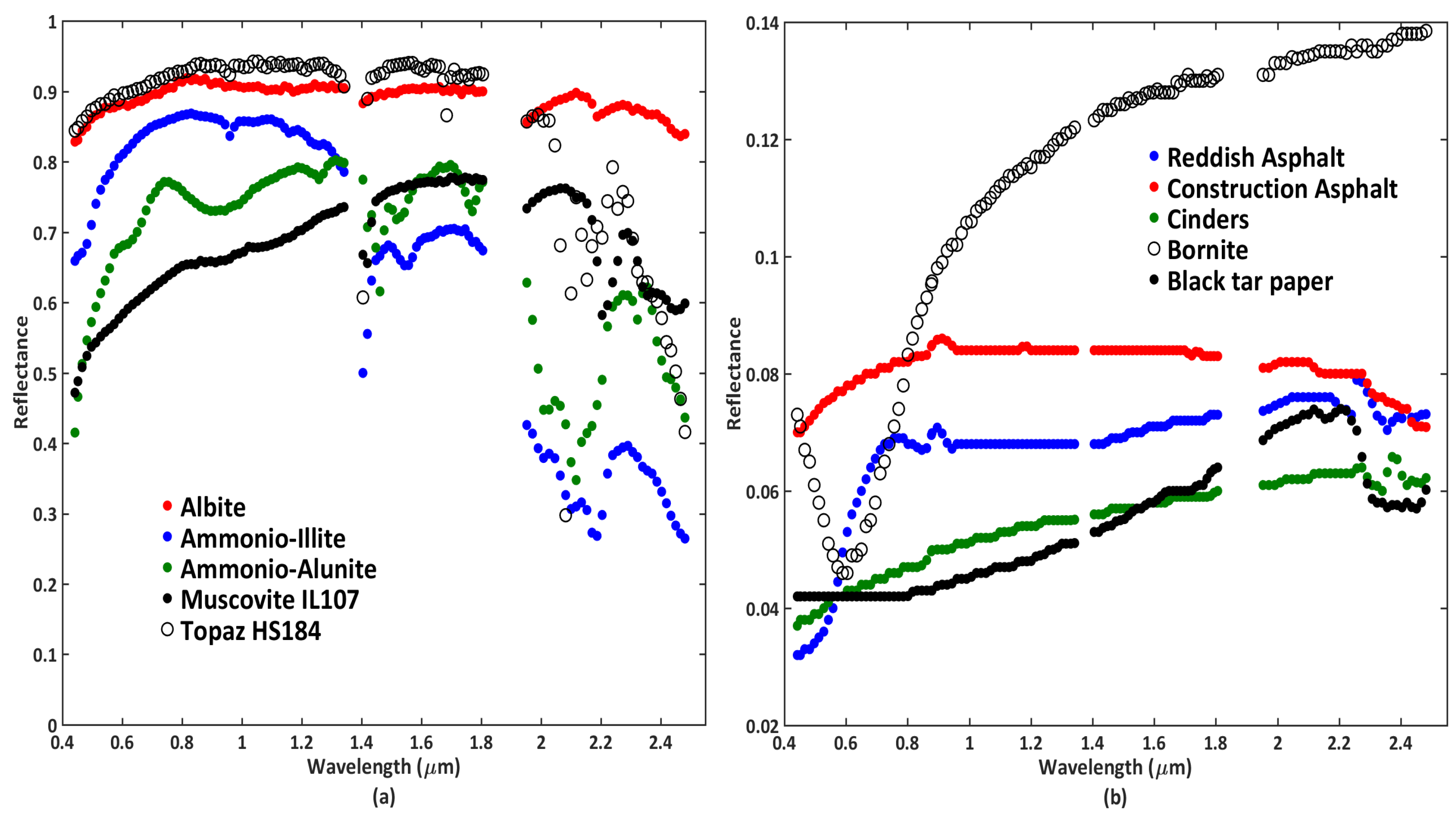
3.3.2. Surfaces with Dark and Bright Materials

This case study aims to analyze the effect of surface albedo on reflectance estimates under high scattering conditions. Two datacubes comprising dark and bright targets are generated respectively. The bright target datacube is generated using spectra of five minerals: Albite, Ammonio-Illite, Ammonio-Alunite, Muscovite, and Topaz. The dark surface is generated mainly using man-made materials: Black tar paper, Cinders, Construction asphalt, Reddish asphalt, and a mineral–Bornite.

The spectra of the materials used to generate the bright and dark surfaces are presented in Figure 6a,b, respectively. The materials used to generate the bright and dark surfaces were physically plausible materials. The choice of the materials ensured that the experiments retrieve atmospheric parameters using realistic bright and dark library spectra that are physically plausible. If the spectra were nonphysical it would not be clear how a real atmospheric retrieval would function.

3.4. Real Data

The purpose of using real sensor data is to validate the proposed method and conclusions from the simulated data under real imaging conditions, i.e., with real sensor noise and scene complexity. The scene used here is an Airborne Prism EXperiment (APEX) sensor datacube (2014) over the Liereman area (within 51.30653${}^{\circ }$ N, 5.013669${}^{\circ }$ E and 51.33816${}^{\circ }$ N, 4.984975${}^{\circ }$ E) in Belgium, shown in Figure 7a. To approximate the size of the simulated image the real scene is cropped into a sub-scene shown in Figure 7b, at the size of the simulated images (100 × 100).

The image of the Liereman area comprises 302 spectral bands between 400 nm and 2500 nm, with a spectral resolution of 4–10 nm depending on the spectral region. Prior to the analysis, bands contaminated by water absorption and low SNR were removed, leaving a total of 227 spectral bands. Further, it is important to note that this data is cloud free. From the spectral analysis of the sub-scene we found that the type of materials present in the scene are comparable to the materials used to generate the synthetic vegetation dataset.

4. The Forward Modeling and the Performance Discriminator

Profiles of the atmospheric condition parameters and their spatial configurations for the forward modeling are given. Two distinct parameters settings are used for experiments with usual scattering conditions (Section 3.2) and for experiments with high scatterings conditions (Section 3.3).

4.1. Profile of the Condition Parameters for the Usual Scattering Conditions

For this purpose, column water vapor value equals 2.0 $\mathrm{g}{\mathrm{cm}}^{-2}$ are used and the sensor altitude is approximately 5 km above sea level resulting in pixel size of 4 m. To obtain a realistic range of AOD for the forward modeling, the method of [25] was applied on three real APEX sensor [45] radiance cubes of the Coast of Belgium. The reason for using the coastal area is its diversity, as the scene is covered by both sea and land. These types of scenes are interesting in terms of determining the uncertainty bounds of AOD for uncertainty exploration as over land and sea AOD shows high variation. This gives us an opportunity to validate the robustness of the proposed methodology for such complexity in the scene.

Estimating a range of AOD is not straightforward with the method of [25] as it provides visibility (in km) as an output. In MODTRAN 4, both AOD and visibility are used to describe the aerosol optical properties. Wherein, visibility scales the aerosol content in the boundary layer (0–2 km). While AOD is a pure number specifying extinction due to aerosols at a specific wavelength $\lambda$. As visibility tends to increase, AOD exponentially decreases. At 550 nm the contributions of molecular depth, ozone depth, trace gases usually are small. Thus, at 550 nm AOD is the main contributor to the total optical depth of the atmosphere i.e., ${\sigma }_e\left(550\right)$ is directly related to the AOD. A high precision in AOD can be achieved by subtracting the Rayleigh scattering coefficient and a very small trace gas depth from a known total optical depth. At 550 nm, visibility is related to AOD by [32],

$$\mathrm{visibility}=\frac{ln\left(50\right)}{{\sigma }_e\left(550\right)+0.01159},$$

(9)

where, 0.01159 ${\mathrm{km}}^{-1}$ is the surface Rayleigh scattering coefficient at 550 nm.

This paper specifically focuses on operational processing chain, where AOD measurements coinciding with image acquisition are often unavailable. Thus, visibility is used to set atmospheric profiles [11,12,13,25,30]. In MODTRAN 4, visibility is given as a parameter for transmittance simulations for a given illumination and viewing geometry. This leads to a look up table of visibility against transmittance. Figure 8a shows the relation between visibility and AOD at 550 nm whereas Figure 8b shows atmospheric transmittance at visibility equals 5, 10, 15, and 20 km. As shown in Figure 8a, the relation between visibility and AOD is exponentially decreasing and the slope is steep for very high scattering conditions that is when visibility is less than 10 km. Care should thus be taken when using visibility to define very high scattering conditions. It is because the relation between visibility and AOD is very sensitive for such conditions and may induce large uncertainty in defining the scattering conditions of the atmosphere.

Further, determining the range of visibility is challenging because the method in [25] is based on the dense dark vegetation (DDV) technique. One of its limitation is that visibility can only be estimated for those pixels. This implies that interpolation is required to estimate visibility for non-DDV pixels. An interpolation method, however, can induce additional uncertainty in a visibility estimation, requiring a separate analysis. To avoid such uncertainty in further analysis, we first recorded all estimations of visibility for the DDV pixels for the entire scene. We then estimated a marginal density of those visibilities (Figure 9). We used kernel methods to estimate the marginal density of visibility [46]. It is implemented using the kde function of the ks package [47] in R [48]. Parameters, for instance, bandwidth and number of modes, used to estimate the marginal densities, are obtained from the h.crit and nr.modes functions as illustrated in the silvermantest package [49,50].

From the marginal density of visibility values as depicted in Figure 9, we observed a skewed distribution, which covers the range between 15 and 120 km. From our experience with the optical parameters in the CDPC, we realized that visibility >60 km has little impact on the estimate of reflectance. Thus, we limit the possible range of visibility to 15 to 65 km, which is approximately equivalent to the AOD range 0.47–0.13.

To simulate the average background radiance for the forward modeling i.e., for the adjacency effect, the spatial relationship is built on the adjacency range (r) values corresponding to the background effect modeling. The average background radiance is as a function of: (1) the extent of the neighborhood or the background window ($EN=(2r+1,2r+1$) of pixels that can spatially influence the target pixel and (2) a weight function within $EN$. Scattering conditions, spatial cross correlation, and uncertainty in estimating r have an influence on pixel wise estimation of $EN$. The optimal value of $EN$ is determined in three steps. First, the minimum value of $EN$ (pre-estimates) is determined by means of variogram fitting using the function vgram.matrix of the fields package in R. Second, a Monte Carlo simulation of photon scattering yielded the relative contribution of $EN$ as a function of AOD, wavelength, aerosol Ångstrom coefficient, anisotropy factor of the Henyey-Greenstein aerosol phase function, the pre-estimated range, and sensor altitude. The photon simulation calculates the cumulative histogram of the adjacency contribution as a function of the distance. Third, using the cumulative histogram, the final $EN$ is determined. To determine the Ångstrom coefficient average AERONET measurements of the Bruges area over the period 2014–2017 are used. Applying this method to the simulated and real scenes, the minimum value of $EN$ was obtained as (41, 41) pixels. The maximum value was set to (91, 91) pixels. This limit was enforced by the spatial extent of the simulated and the real sub image (100 × 100 pixels).

4.2. Pixelwise Parameter Configuration for the Usual Scattering Conditions

From the ranges of visibility and $EN$, we derive their spatial pattern or variability over each pixel, as we may find in real scenes, for the forward modeling. For the simulated datasets, a gradual increase in visibility which varies between 15 km and 65 km corresponding to an AOD range 0.47–0.13 was realized. The direction of variation is taken from the left of the simulated images to the right, i.e., column wise, with a step size of 2 km. To each pixel in a column, randomly sampled values from the log–normal ($\mu$, 0.02) with $\mu =$ 15 km for the first column are assigned. A log-normal distribution is used to approximate the actual distribution of visibility, being a skewed normal distribution (Figure 9). The resultant spatial variability of visibility is shown in Figure 10a.

For the adjacency effect, we considered the spatial variability of the classes present in the simulated image (Figure 2b). From visual interpretation we found that the spatial variability is spectrally more homogeneous at the center of the image than at the edges and becomes more heterogeneous at the edges. This is because of the spatial variability of the materials present in the scene, as shown in Figure 3. A significant influence on the center pixels is thus likely caused by pixels that are far away from the center, because spectrally homogeneous pixels cause a low adjacency effect. To address this spatial variability we set a large adjacency range $EN$ = 91 pixels at the center of the image that gradually decreases to $EN$ = 41 pixels at the edges (Figure 10b).

4.3. Profile of the Parameters for the High Scattering Conditions

Parameters setting for the experiments with high scattering conditions are given in

Table 1. Visibility and corresponding AOD values considered as true values for experiments with high scattering conditions with column water vapor equals 2.0 g cm${}^{-2}$.

True Visibility (km)	True AOD
1	4.94
4	1.42
7	0.89
10	0.68
15	0.48

. These values are considered as true values for the analyses. Using these values the forward modeling is performed and at-sensor radiance cubes are obtained for: spectrally similar and distinct dataset and dark and bright datasets.

4.4. Performance Discriminators

The quantitative assessment of the propagation of uncertainty originating from the AC parameters is measured by the signal to reconstruction error SRE $\equiv \frac{E\left[{\parallel x\parallel }_2^2\right]}{E\left[\parallel x-\widehat{x}{\parallel }_2^2\right]}$, where x is the reference signal and $\widehat{x}$ represents its estimation. SRE provides information on the power of the signal with respect to the power of the error [51]. In all experiments, we report SRE measured in dB: SRE (dB) = 10${\log }_{10}\left(\mathrm{SRE}\right)$.

5. Estimation

5.1. Linear Model for Calibration

In a hyperspectral datacube each pixel is represented with a vector of length B denoting the number of channels. Further, the true reflectance ${\rho }_{\mathrm{t}}$ of the underlying surface within the IFOV is affected by atmospheric absorption and scattering. Then its estimate ${\widehat{\rho }}_{\mathrm{t}}$ obtained via AC is expressed as a linear model:

$${\widehat{\rho }}_{\mathrm{t}}=\mathbf{C}·{\rho }_{\mathrm{t}}+n,$$

(10)

where the matrix $\mathbf{C}\in {\mathbb{R}}^{B\times B}$, is assumed to be diagonal, stores coefficients that model the deviation of ${\widehat{\rho }}_{\mathrm{t}}$ from ${\rho }_{\mathrm{t}}$ and n is the noise effect.

If the coefficients of $\mathbf{C}$ approach 1 then the estimates of AOD approach the actual AOD at the time of imaging, indicating a perfect match. If, however, the coefficients of $\mathbf{C}$ deviate from 1, then the error in the estimates of AOD increases. Here, we assumed that the effect of other atmospheric parameters such as column water vapour is absent.

Fitting the linear model (Equation (10)) by least squares is equivalent to an $l_2$–norm optimisation problem where the deviation in the coefficients of $\mathbf{C}$ is minimised. In fact, it minimises the sum of the squares of the differences between ${\widehat{\rho }}_{\mathrm{t}}$ and ${\rho }_{\mathrm{t}}$:

$$\underset{\mathbf{C}}{min}\frac{1}{2}\parallel \mathbf{C}·{\rho }_{\mathrm{t}}-{\widehat{\rho }}_{\mathrm{t}}{\parallel }_2^2,$$

(11)

5.2. Searching for Reference Library Spectra

To generate pre-estimates of reflectance, we executed AC for k different visibility values that generated k reflectance cubes. As ${\rho }_{\mathrm{t}}$ is not known a priori, we need its estimation that serves as a reference to solve Equation (11). Here, we assume that the ${\rho }_{\mathrm{t}}$ contains materials that are available in a spectral library, which is known a priori. Spectral unmixing of the k reflectance cubes provides k abundance maps indicating the fractional coverage of material present in each pixel. For unmixing realised through the linear mixture model, ${\rho }_{\mathrm{t}}$ can be expressed as a linear combination of the spectra of the endmembers, weighted by their abundances:

$${\rho }_{\mathrm{t}}=y=\mathbf{A}·x+N.$$

(12)

Here, $\mathbf{A}\in {\mathbb{R}}^{B\times m}$ is the set of endmembers in the scene serving as a spectral library containing m pure spectra, $x\in {\mathbb{R}}^m$ is the vector of corresponding fractional abundances compatible with $\mathbf{A}$, and $N\in {\mathbb{R}}^B$ is a noise vector. In this article, we assume that $\mathbf{A}$ is available a priori. Unmixing thus aims at identifying the atoms of $\mathbf{A}$ which are active in each pixel and their respective abundances. From the works of [27,52], we found that Sparse Unmixing via Variable Splitting, Augmented Lagrangian and Total Variation (SUnSAL-TV) [52] a better option than SUnSAL without TV [51] for unmixing in the presence of noise. SUnSAL-TV takes intrinsic spatial smoothness into account as an important characteristic of natural scenes. We thus use SUnSAL-TV to obtain a solution with piece wise smooth transitions of the abundance fractions in neighbouring pixels. SUnSAL-TV solves the optimization problem:

$$\underset{X}{min}\frac{1}{2}{\parallel AX-Y\parallel }_F^2+{\lambda }_1{\parallel X\parallel }_{1,1}+{\lambda }_{TV}\mathrm{TV}\left(X\right),$$

(13)

where

$$\mathrm{TV}\left(X\right)\equiv \sum _{\{i,j\}\in \epsilon }{\parallel x_i-x_j\parallel }_1$$

(14)

is a vector extension of the non-isotropic TV [53] and $\epsilon$ denotes the set of neighbours in the image. In Equation (13), $\mathbf{Y}\in {\mathbb{R}}^{L\times n}$ is the observed data matrix with each column containing the observed spectrum at a pixel, $\mathbf{X}\in {\mathbb{R}}^{m\times n}$ is the matrix of fractional abundances, ${\parallel \mathbf{X}\parallel }_F\equiv \sqrt{\mathrm{trace}\left\{{XX}^T\right\}}$ represents the Frobenius norm of $\mathbf{X}$ and ${\parallel \mathbf{X}\parallel }_{1,1}\equiv {\sum }_{i=1}^n{\parallel x_i\parallel }_1$, with $x_i$ denoting the ith column of $\mathbf{X}$. The first term in Equation (13) measures the data misfit, the second term forces the matrix of fractional abundances to be sparse, and the last term accounts for spatial homogeneity of the abundance maps. The parameters ${\lambda }_1\ge 0$ and ${\lambda }_{TV}\ge 0$ are regularization parameters. SUnSAL-TV introduces a set of new variables per regularizer and then uses the Alternating Direction Method of Multipliers (ADMM) [54] to solve the resulting constrained optimization problem. In our experiments, we neglect sparsity as the spectral libraries employed will contain a small number of endmembers. We use SUnSAL-TV applying both the non-negativity constraint (ANC) and the sum to one constraint (ASC) [55] to solve the optimization problem (Equation (13)). Only spatial information is considered in SUnSAL-TV by setting ${\lambda }_1=0$ and ${\lambda }_{TV}$ >0. The ASC, often ignored due to signature variability [56] is used in this work as we assumed the set of image endmembers to be known and hence no sparsity is enforced on the vectors of abundances. The sparsity indicates that only a small number of endmembers are present inside a pixel and implies that only a few endmembers contribute to y, which is true for high resolution images.

5.3. Generating the First Visibility Estimate

The methods then identifies the locations of pure pixels in the k reflectance cubes using the unmixing method discussed in Section 5.2. The retrieved abundance maps are, however, contaminated by retrieval uncertainties of the observed surface, atmospheric parameters, and instrumental errors. To accommodate for these uncertainties we select pure pixels in the k reflectance cubes with an abundance value between $1-t_1$ and 1.0, where $t_1$ indicates a threshold value that can be set according to the target application and the sensor configurations. The spectra of each pure pixel are then evaluated for distortion in terms of shape as can be determined by the spectral angle mapper. The smaller the spectral angle the more similar a pixel is to a given library spectra. The corresponding visibility value providing the minimum spectral angle value and minimizing (Equation (11)) in least square terms is considered as estimates of visibility for the reference pixel.

5.4. Iterations

Using the pre-estimates of visibility, we re-estimate $\widehat{{\rho }_{\mathrm{t}}}$ by minimizing the $\mathbf{C}$ iteratively. We derive a new visibility value $D_{{\mathrm{vis}}_{i,e+1,\lambda }}$ for pixel i as

$$D_{{\mathrm{vis}}_{i,e+1,\lambda }}=\left\{\begin{array}{cc}{D}_{{\mathrm{vis}}_{i,e,\lambda }}+q,\hfill & \mathrm{if}C(\lambda ,i)<1-t_2\hfill \\ D_{{\mathrm{vis}}_{i,e,\lambda }}-q,\hfill & \mathrm{if}C(\lambda ,i)>1+t_2\hfill \\ D_{{\mathrm{vis}}_{i,e,\lambda }},\hfill & \mathrm{otherwise}\hfill \end{array}\right.$$

(15)

where e is the iteration, $D_{{\mathrm{vis}}_{i,e,\lambda }}$ is incremented or decremented by q depending on the conditions whether $\mathbf{C}$ is greater or less than the threshold value set by $t_2$. In this way, Equation (11) is iteratively solved unless coefficient of $\mathbf{C}$ are close to 1.0. We use the coefficient range between $(1-t_2)$–$(1+t_2)$ as a convergence criterion.

5.5. Interpolation of Visibility

Following step 5.4, we obtained visibility values for the reference pixels, a spatial estimation method is applied to pixels that are spatially related to the reference pixels. A choice of spatial estimation method depends on the type of surface, number of reference pixels, and size of the scene. The optimal number of neighboring points to be used for spatial estimation depends on the adjacency range (r) values corresponding to the background effect modeling. Three cases are distinguished to take account of the spatial locations of the reference pixels and to select spatial estimation method:

• Case 1: No overlapping of the neighborhood. This case accounts for the scenario when within the neighborhood of the target reference pixel $E{N}_{\mathrm{target}}$, no other reference pixel fall.
• Case 2: Overlapping of the neighborhood. This case accounts for scenarios when the neighborhood of two or more reference pixels overlaps with $E{N}_{\mathrm{target}}$. This occurs when two or more pixels falls within $E{N}_{\mathrm{target}}$.
• Case 3: No reference pixel is available for spatial estimation. This case account for the scenario when to estimate visibility at the unsampled location, no reference pixel can be spatially linked using $EN$.

To solve Case 1, stationarity is assumed within $E{N}_{\mathrm{target}}$ implying the parameters, such as mean and variance, are same in all parts of $E{N}_{\mathrm{target}}$ and in all directions. Randomly sampled values from $P(\mu ,\sigma )$ distribution are used to assigned values within $E{N}_{\mathrm{target}}$. Here, $\mu$ is the value of visibility at the reference pixel and $\sigma$ is used to accommodate for the insignificant spatial variability in visibility.

To solve Case 2, if w number of neighborhoods $E{N}_1,\dots ,E{N}_{\mathrm{w}}$ are overlapping then the pixels within $E{N}_1,\dots ,E{N}_{\mathrm{w}}$ are combined to create a large field accommodating all the overlapping reference pixels. An interpolation is then applied on this large field using values of visibility at all the accommodated reference pixels as data points.

To solve Case 3, for a pixel that is spatially unrelated to any reference pixel, visibility value is estimation using a method, which is called binning. Binning comprises the following steps:

• Step 1, find the spatial variation of visibility using values estimated for Case 1 and Case 2. We distinguished three types of spatial variation in visibility: (a) vertical; (b) horizontal; and (c) diagonal. The specific variation is obtained by evaluating histograms of visibility values from line transects in vertical, horizontal, and diagonal directions. A bimodality or multimodality of the histogram from a specific line transect shows a strong variation of the visibility. For instance, if visibility is vertically varying (column wise) then the histogram obtained from the horizontal line transect shows bimodality or multimodality,
• Step 2, the histogram that shows unimodality, that is direction of non-variation of visibility, is used to generate the distribution $P(\mu ,\sigma )$. For instance, if visibility is vertically varying then histogram generated from the values from vertical line transect are used to generate the $P(\mu ,\sigma )$,
• Step 3, for vertical and horizontal variation, a randomly sampled value from $P(\mu ,\sigma )$ is assigned to a spatially unrelated pixel. If visibility is diagonally varying then nearest neighborhood method [57] is used to interpolate the missing value.

6. Results of Experiments with Usual Scattering and with Real Data

6.1. Specific Choices of Methods and Values

The value of k is set to three and visibility values, 35, 45, and 55 km that generated three reflectance cubes are used. The values between 35 and 55 km (AOD values between 0.22 and 0.14) correspond to moderate scattering conditions, which suits to the imaging conditions of airborne campaigns. The value of $t_1$ is set to 0.05 resulting in fraction between 0.95 and 1.0 as a criterion to select a pure pixel. From our experience with real images processed through the CDPC we learned that a reflectance estimate is not sensitive to visibility values that are less than 5 km. Therefore, to solve Case 1, we set $\sigma =2.5$. To solve Case 2, we used a weighted average inverse distance to power method with power equal to 2 [57,58]. To solve Equation (15), we set $q=5$ km as reflectance is sensitive to a difference of 5 km in visibility value. The convergence criterion is set between 0.99 and 1.01 by setting $t_2$ to 0.01. Such a narrow range allows estimating the finest achievable visibility value of a sensor. Depending on the end product and sensor configurations, wider convergence ranges can be explored.

6.2. Visibility Estimation for the Simulated Dataset

In Figure 11, visibility estimates with 30 dB correlated noise before binning are shown in Figure 11a and after binning in Figure 11b, for the sixth iteration. The spatial variability of the estimated visibilities after binning were comparable to that of the true visibilities (Figure 10a). This is confirmed from the direction of variation of the visibility estimates which is from the left to the right, i.e., column wise as that of the true visibilities. Further, the performance of the proposed method was evaluated from the range of the estimated visibilities after binning and their pixelwise absolute differences (Figure 11c) with true visibilities. For most of the pixels the difference was less than 10 km and only for 805 pixels out of 10,000 pixels the difference was greater than 10 km. This implies that approximately 8% pixels had severely affected the reflectance estimates after the sixth iteration. With more iterations the performance was further improved but could not linearly improve the reflectance estimates. This could be attributed to high noise level. For lower noise levels however, the performance was further improved with percentage of pixels above 10 km limited to approximately 2%.

We then estimated reflectance using visibility values after binning (Figure 11b) and observed a significant improvement in the estimations of reflectance from iteration 1 to iteration 6. We observed a performance (SRE) of 35 dB after six iterations. After more iterations, however, further changes in visibility did not improve reflectance estimations. This could be attributed to the high noise level. Further, a distinction between visibility values within a small interval of 5–7 km, which corresponds to AOD values between 0.06 and 0.08, was difficult to observe from the coefficient values. This is because of the relatively low sensitivity of reflectance to visibilities within that interval. This is consistent with our previous work [27]. To obtain these results, the optimal value of ${\lambda }_{TV}$ corresponds to the maximum value of SRE (dB) was 0.01 for 30 dB noise case. For all other noise levels the optimal value of ${\lambda }_{TV}$ was 0. This implies that ${\lambda }_{TV}$ is a suitable regularization parameter under the high noise condition.

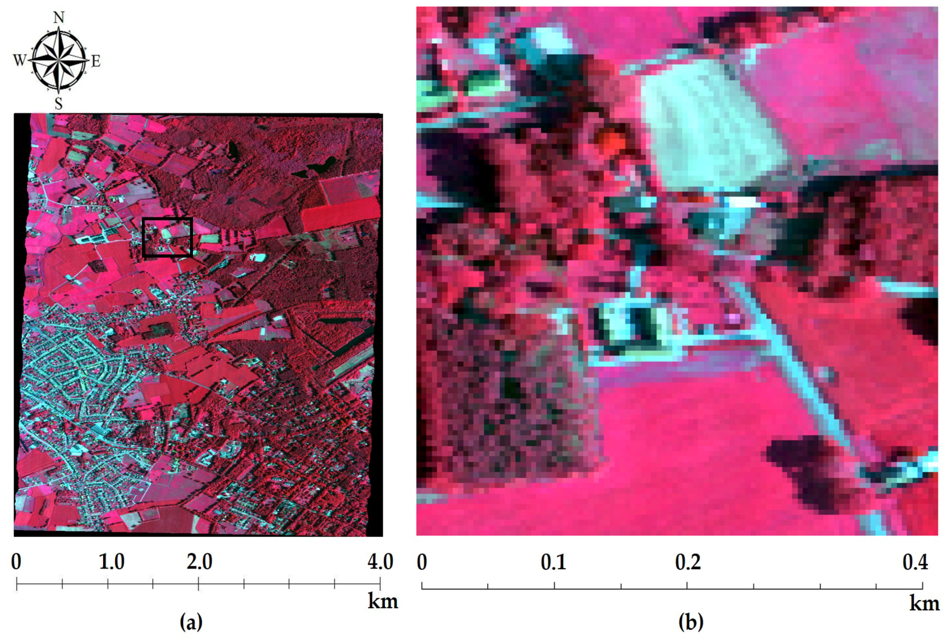
6.3. Visibility Estimation for the Real Dataset

For the real dataset, we cannot evaluate the performance of the method as there is no reference dataset available. Thus, we considered generating a pseudo reference dataset. To achieve this, we perform additional pre-processing on the available real reflectance cube (Figure 7). The procedure to generate the reference reflectance cube comprises the following steps:

• From the real at sensor radiance cube, a set of endmembers is manually selected, whereas the corresponding pixels are called reference pixels.
• Reflectance are estimated by performing AC using various pre-selected combinations of the atmospheric condition parameters.
• From the estimated reflectance cubes spectra of the reference pixels are evaluated to check distortion in terms of shape (Section 5.3).
• The reflectance cube that corresponds to the optimal combination serves as the reference cube.
• The reference cube is transformed to obtain a pseudo at sensor radiance cube using the MODTRAN 4 forward modelling simulations with the same atmospheric conditions as used in the forward modelling of the simulated dataset.
• To the pseudo reference dataset we added 60 dB white Gaussian noise at sensor level and 30 dB correlated noise to the estimated reflectance cube, as we did for the simulated dataset.

Figure 12 shows estimations of visibility after the second and fifth iterations. After five iterations we observed a saturation in performance and observed a performance (SRE) of 35 dB. This implies that further improving visibility estimates would not improve reflectance estimates. We observed results of estimating visibility which are similar to the findings with the simulated dataset. The optimal value of ${\lambda }_{TV}$ corresponds to the maximum value of SRE (dB) is 0.01 for 30 dB noise case. Further, in Figure 12c,d the pixelwise absolute difference between true visibility values (Figure 10a) and visibility estimates after second and fifth iteration are shown respectively. After two iterations the number of pixels with the difference value higher than 10 km was 2191 pixels which was reduced to 1397 pixels after five iterations. This implies that approximately 22% and 14% pixels had severely affected the reflectance estimates after second and fifth iterations, respectively. With more iterations the performance was further improved but it did not linearly improve the reflectance estimates. This could be attributed to high noise level and to the sensitivity of reflectance to visibility values. As found from the experiments with the synthetic datasets. For lower noise levels however, the performance was further improved with percentage of pixels above 10 km came down to approximately 2–3%.

For performance assessment, we compared our method with the DDV pixels-based visibility estimation method in [25]. Applying the DDV method on both the datasets we obtained visibility at DDV pixels only. Further, the DDV-based method is highly effected by illumination and viewing geometry even for the same flight line. We observed large variation in visibility estimation for adjacent pixels. For instance, at one pixel the estimated value was 32 km whereas at the next pixel it was 80 km. Because of large variation, low SRE (between 5 and 10 dB) was observed at the DDV pixels. From these results we conclude that the proposed method performs better than the reference method.

6.4. Experiment with Spatial Variability

This experiment aims to test the proposed method for different spatial variability of visibility and adjacency range. The spatial variations in the parameters are achieved by applying rotation to the reference values of visibility and the background window size defined for each pixel in Figure 10a,b. We also applied spatial smoothing to visibility values at each pixel after the rotation. In addition, visibility and background window are varied diagonally, see Figure 13, Figure 14, Figure 15 and Figure 16. The reason to rotate and smooth the reference data and to realise diagonal variability, is to generate different ways to arrange visibility and adjacency in the spatial domain. These variations of the parameters cover some relevant variation scenarios as can be found in real imaging conditions. These spatial variations are used in the forward modelling as explained in Section 4.2 to obtain various at sensor radiance cubes. The proposed method is then applied on the at sensor radiance cubes. The measured SRE values are close to 35 dB. In addition, the number of iterations to achieve convergence is between 5 and 7. This experiment showed that the method presented in this article estimates visibility correctly for various spatial variation of the parameters.

7. Results of Experiments with High Scattering Conditions

Specific Choices of Methods and Values

A univariate analysis is performed to analyze the effect of scattering and surface albedo on a quality of spectra. Reflectance is estimated with a set of visibility values that are deviated from their true values (Table 1). From the experiments with the usual scattering conditions, we found that an estimation of visibility is not sensitive to a small variation in visibility values (between 5 and 7 km). Thus, we deviate visibility values within ±4–6 km range. The specific values used for reflectance estimates and their corresponding true values are given in

Table 2. True visibility values and visibility values used for estimating reflectance, and corresponding AOD values with column water vapor equals 2.0 g cm${}^{-2}$.

True Visibility (km)	Set Visibility (km)	True AOD	Set AOD
01	05	4.94	1.17
04	01	1.42	4.94
04	10	1.42	0.68
07	02	0.89	2.60
07	12	0.89	0.57
10	05	0.68	1.17
10	15	0.68	0.48
15	10	0.48	0.68
15	20	0.48	0.37

. Further, to separate the noise effect from the scattering and albedo effects, only 60 dB correlated noise (no random noise) is added to the datasets.

Using the visibility values given in Table 2, reflectance estimates were obtained. Subsequently, SUnSAL-TV method (13) was applied for estimating fractional abundances. The optimal values of ${\lambda }_1$ and ${\lambda }_{\mathrm{TV}}$ were found to be 0. In Figure 17, the effect of high scattering on reflectance estimates and on abundance estimates are shown. From these performance plots we observed that other than uncertainty in atmospheric condition parameters, surface albedo was the important factor in determining performances at both reflectance and unmixing levels. Further, the maximum achievable performances at unmixing level was just above 25 dB compared to 42 dB at reflectance level. This could be attributed to limitations of the unmixing method.

In Figure 18 and Figure 19 the effects of scattering and variation in visibility values on spectral qualities of materials used to generate spectrally distinct and spectrally similar datasets, respectively are shown. Setting the visibility higher and lower than the true visibility resulted in overestimation and underestimation of reflectance, respectively. This pattern is clearly visible in these figures. For instance in Figure 18e. The overestimation and underestimation pattern reverses for low albedo targets i.e., targets with reflectance less than 0.25%. The incorrect scattering conditions had further distorted the shape of the spectra especially at strong water vapor absorption features. For instance, as shown in Figure 18a. This could be attributed to the physical relation between aerosols and water vapor in the atmosphere and to the low SNR at water absorption features.

Likewise, for dataset generated with spectrally similar materials (Figure 19) similar results were observed as for the dataset generated with spectrally distinct materials (Figure 18). In addition, negative reflectance estimates were observed when scattering conditions were overestimated. Under those conditions when surface albedo were low (0.2%), the proportion of $L_{\mathrm{pa}}$ in $L_{\mathrm{rs},\mathrm{t}}$ was higher than $L_{\mathrm{t}}$. For such scenarios the reflectance estimates via AC resulted in negative estimates.

In Figure 20, the effects of surface albedo, scattering, and variation in visibility on spectral qualities of bright and dark target datasets are shown. Other than the effect of variation in defining scattering conditions, the effect of surface albedo was more prominent for these results. Especially, the negative estimations of reflectance and high variation in reflectance estimates were observed. These results were further confirmed with the results shown in Figure 17.

8. Discussion

This article presents a method that iteratively estimates aerosol optical depth (AOD) from the estimates of reflectance spectra. It was applied to a hyperspectral sensor and there is no reason why it should also not be effective on other hyperspectral sensors. The method is simple to implement and can be extended to encompass other atmospheric parameters. In particular, the number of iterations for a pixelwise estimation is between 6 and 8. The reason why we could use less iterations is that for each iteration the new estimates are fed back into atmospheric correction procedures where estimation converges when reflectance becomes insensitive to changes in visibility. This is in contrast to those AOD estimation methods which were developed empirically or developed for a specific surface characteristics or developed with a relation between bands in near-infrared, red, and blue wavelength regions [25,59,60,61,62,63]. Further, a common approach to estimate AOD is to use at-sensor radiance where AOD is derived at specific wavelengths either using some band relation or using in situ point measurements coinciding with spaceborne or airborne imagining. For instance, many AOD estimation methods use ground measurements such as AERONET sites or sun photometer and derive AOD at specific wavelengths and later interpolate AOD for other wavelengths [61,64]. Such methods however ignore uncertainty arising from Ångstrom coefficient or uncertainty arising from the wavelength mismatch of in situ instrument and sensor wavelengths. For methods built on such specific relations it is not possible to encompass other atmospheric condition parameters. Important to note that it was impossible to compare our AOD estimation method with the common practice of using at-sensor radiance to estimate AOD at every point. The reason is that that our method uses surface reflectance and therefore the comparison was restricted to a limited evaluation.

The proposed method was applied on a small sub-scene to differentiate between uncertainty and variability of the scene. This way larger real scenes divided into smaller sub-scenes can be processed. The only challenge there would be to estimate background contribution for adjacency correction. It is because in larger scenes background radiance can originate from pixels that are outside the sub-scene, especially for spaceborne data. This challenge can be resolved by first estimating the background contribution over the full scene. In the literature, most of the AOD estimation methods do not estimate AOD for each pixel. Instead AOD values are derived for specific surface types which can be dark surface or dense dark vegetation pixels [25,60,62]. In contrast to those methods our method estimates AOD using reflectance at each pixel with a relation between adjacency range function and scattering conditions and acknowledges the uncertainty arising from this relation.

For initial estimates of reflectance, we considered 35, 45, and 55 km values of visibility for AC that generated three reflectance cubes. The range of values between 35 and 55 km (AOD values between 0.22 and 0.14) serves as a good preliminary range because airborne campaigns are often performed under low to moderate scattering conditions. This value can, however, be adjusted for spaceborne data or when the data is acquired under high scattering conditions. The proposed method is flexible for such changes as it uses reflectance estimates at each pixel to derive AOD. The methods which iteratively use reflectance estimates to derive AOD either do not estimate AOD at each pixel or are sensitive to viewing and illumination geometry. For instance, the method of [59] uses iterative estimations of reflectance to infer AOD values but their estimations are highly sensitive to viewing and illumination geometry. To compensate for such effects, average value of 10 pixels by 10 pixels were used. In contrast to those methods, our method acknowledges uncertainty arising from viewing and illumination geometry and iteratively minimizes those uncertainty during AOD estimates.

The interpolation method used in this study is weighted average inverse distance to power method. This choice is based on the assumption that for a small scene pixels that are close to the target pixel are contributing more to the background radiation than those that are farther apart. Moreover, for small area the choice of the interpolation method is not critical. Further, any uncertainty arising from the interpolation method is tractable. It is because the spatial extent of neighboring pixels is based on an adjacency range, which is calculated using the three step process defined in Section 5.4. While performing experiments for different spatial variations of the two parameters, low performance was expected when visibility was diagonally varying, especially to solve Case 3. We hypothesized that the nearest neighbor method could affect the performance of the method for various diagonal variations (as shown in Figure 13, Figure 14, Figure 15 and Figure 16). However, no notable variation in the performance was observed. This is attributed to the small area where choice of the interpolation method was not critical. More experiments can be performed to test the effect of spatial variation on the performance for larger scenes. As for the small area the choice of interpolation method is not critical, the choice of the interpolation method made in this article is based on the computation speed. For instance, the nearest neighbor interpolation method is faster than the cubic or spline-based interpolation methods.

The criterion to select pure pixels is based on the value of $t_2$ and the spectral angle values. To further automate this process factors such as scattering conditions, scene heterogeneity, path length from surface to the sensor can be considered and more sophisticated methods that identify reference pure pixels under uncertainty can be developed.

Care should be taken when using visibility as a substitute to AOD, especially under high scattering conditions where AOD is highly sensitive to visibility. As long as airborne campaigns are not acquired under high scattering conditions, errors seen at visibility 0–10 km as in [65] are unlikely to be experienced with operational remote sensing.

From the performance of reflectance and abundance estimates under high scattering conditions with the albedo effects, as sown in Figure 17, we observe that the overall performance of abundance estimates are lesser than the performance of reflectance estimates. This might be due to the inherent limitations of the unmixing method, their numerical approximations, and the non-linear propagation of uncertainty from visibility to abundance estimates via AC. Further, the performances of reflectance and abundance estimates for bright surface and for dataset with spectrally distinct materials are higher than the performances for dark surface and for dataset with spectrally similar materials. Bright targets reflect more radiation energy than dark targets. Thus, for the bright targets the majority of the at-sensor radiance consists of photons that are not scattered. In contrast, most of the photons for the dark targets are scattered [27,66]. This contribution amplifies under high scattering conditions resulting in performance degradation.

As established in the literature, a variability in aerosol optical depth affects the amplitude of the retrieved spectra. This influence was not linear, in the sense that deviations from the reference spectra depend on the surface reflectance of the target, the wavelength, and the scattering conditions [6]. This observation is consistent with our previous work [26,27]. For high aerosol optical depth values and high surface reflectance (>$0.3$), the estimated reflectance was higher than the reference reflectance, whereas for low surface reflectance (<$0.3$) estimated spectra were lower than reference spectra. This consistently happened for spectra of all considered endmembers. An opposite pattern was observed for low scattering conditions. In [67], a threshold $P_c=\frac{\mathrm{AOD}}{{\rho }_t\left(\lambda \right)}$ was introduced as a critical parameter to determine how the estimated reflectance changes due to aerosol scattering. Applying this threshold we found that if $P_c$ > 1, then the estimated surface reflectance was underestimated, otherwise it was overestimated. The changes in the estimated reflectance were negligible when aerosol optical depth approaches the reflectance value. Considering these effects, the results of all nine visibility combinations (Table 2) are not shown in Figure 18, Figure 19 and Figure 20. It is because for extremely high scattering conditions reflectance estimates are either significantly overestimated or underestimated, (especially in the blue wavelength region) which may bias the analyses. As discussed earlier, the airborne remote sensing is not performed under such high scattering conditions. However, the analyses give a useful insight into the effect of those conditions on the spectral quality of the data and ultimately to the performance of the proposed method. These results might be useful to spaceborne data.

9. Conclusions and Outlooks

The experiments reported in this article have four components: atmospheric correction (AC), retrieval of visibility, unmixing to extract locations of pure materials, and propagation of uncertainty from visibility to reflectance estimates. A sensitivity analysis provided information on the contribution of sources of variation to dispersion in the output. A distinction in visibility between 5 and 7 km, corresponding to AOD values between 0.06 and 0.08, is difficult to obtain from the coefficient values because of the relatively low sensitivity of reflectance to variability in visibility. We therefore conclude that sensitivity of an application product to uncertainty in a parameter is useful as a convergence criterion while estimating the involved parameters.

The uncertainty propagation analysis showed that an estimate of the atmospheric condition parameter visibility using reflectance is more efficient than using at-sensor radiance. Sources of uncertainty and propagation of uncertainty are useful measures to determine the performance of an estimation method. The experiments using high scattering showed that a deviation in visibility from its true value affected the reflectance estimate. Hence, an uncertainty analysis is important to assess the performance of an estimation method as well as of a model that uses reflectance as an input. Also, the surface albedo is an important source of uncertainty for estimating a parameter and for quantifying the propagation of uncertainty. Experiments with dark and bright surface show that the surface albedo influences the quality of the spectra retrieved via AC, independently from other effects.

The present study can be further extended to take other atmospheric correction parameters into account. Deeper effects of the Ångstrom coefficient can be investigated. It would be interesting to use the proposed method if various methodological choices have to be fine-tuned. Experiments with spectral libraries containing a large number of spectral signatures are recommended but those are beyond the scope of the current study.

References

1. Jarocinska, A.M.; Kacprzyk, M.; Marcinkowska, A.; Ochtyra, A.; Zagajewski, B.; Meuleman, K. The application of APEX images in the assessment of the state of non-forest vegetation in the Karkonosze Mountains. Misc. Geogr. 2016, 20, 21–27. [Google Scholar] [CrossRef] [Green Version]
2. Tagliabue, G.; Panigada, C.; Colombo, R.; Fava, F.; Cilia, C.; Baret, F.; Vreys, K.E.A. Forest species mapping using airborne hyperspectral APEX data. Misc. Geogr. 2016, 20, 28–33. [Google Scholar] [CrossRef] [Green Version]
3. Mierczyk, M.; Zagajewski, B.; Jarocińska, A.; Knapik, R. Assessment of Imaging Spectroscopy for rock identification in the Karkonosze Mountains, Poland. Misc. Geogr. 2016, 20, 34–40. [Google Scholar] [CrossRef] [Green Version]
4. Krówczyńska, M.; Wilk, E.; Pabjanek, P.; Zagajewski, B.; Meuleman, K. Mapping asbestos-cement roofing with the use of APEX hyperspectral airborne imagery: Karpacz area, Poland—A case study. Misc. Geogr. 2016, 20, 41–46. [Google Scholar] [CrossRef]
5. Demarchi, L.; Canters, F.; Cariou, C.; Licciardi, G.; Chan, J. Assessing the performance of two unsupervised dimensionality reduction techniques on hyperspectral APEX data for high resolution urban land-cover mapping. ISPRS J. Photogramm. Remote Sens. 2014, 87, 166–179. [Google Scholar] [CrossRef]
6. Seidel, F.C.; Kokhanovsky, A.A.; Schaepman, M.E. Fast retrieval of aerosol optical depth and its sensitivity to surface albedo using remote sensing data. Atmos. Res. 2012, 116, 22–32. [Google Scholar] [CrossRef]
7. Bhatia, N.; Stein, A.; Reusen, I.; Tolpekin, V.A. An optimization approach to estimate and calibrate column water vapour for hyperspectral airborne data. Int. J. Remote Sens. 2018, 39, 2480–2505. [Google Scholar] [CrossRef]
8. Popp, C.; Brunner, D.; Damm, A.; Roozendael, M.V.; Fayt, C.; Buchmann, B. High-resolution NO2 remote sensing from the Airborne Prism EXperiment (APEX) imaging spectrometer. Atmos. Meas. Tech. 2012, 5, 2211–2225. [Google Scholar] [CrossRef]
9. Gao, B.C.; Davis, C.; Goetz, A. A Review of Atmospheric Correction Techniques for Hyperspectral Remote Sensing of Land Surfaces and Ocean Color. In Proceedings of the 2006 IEEE International Symposium on Geoscience and Remote Sensing, Denver, CO, USA, 31 July–4 August 2006; pp. 1979–1981. [Google Scholar]
10. Gao, B.C.; Montes, M.J.; Davis, C.O.; Goetz, A.F. Atmospheric correction algorithms for hyperspectral remote sensing data of land and ocean. Remote Sens. Environ. 2009, 113, S17–S24. [Google Scholar]
11. Richter, R.; Schlapfer, D. Atmospheric/Topographic Correction for Airborne Imagery (ATCOR-4 User Guide); User Guide; DLR-German Aerospace Center: Köln, Germany, 2007. [Google Scholar]
12. Biesemans, J.; Sterckx, S.; Knaeps, E.; Vreys, K.; Adriaensen, S.; Hooyberghs, J.; Meuleman, K.; Kempeneers, P.; Deronde, B.; Everaerts, J.; et al. Image processing work flows for airborne remote sensing. In Proceedings of the 5th EARSeL Workshop on Imaging Spectroscopy. European Association of Remote Sensing Laboratories (EARSeL), Bruges, Belgium, 23–25 April 2007. [Google Scholar]
13. Sterckx, S.; Vreys, K.; Biesemans, J.; Iordache, M.; Bertels, L.; Meuleman, K. Atmospheric correction of APEX hyperspectral data. Misc. Geogr. 2016, 20, 16–20. [Google Scholar] [CrossRef]
14. Diner, D.J.; Martonchik, J.V.; Kahn, R.A.; Pinty, B.; Gobron, N.; Nelson, D.L.; Holben, B.N. Using angular and spectral shape similarity constraints to improve MISR aerosol and surface retrievals over land. Remote Sens. Environ. 2005, 94, 155–171. [Google Scholar] [CrossRef]
15. North, P.R.J. Estimation of aerosol opacity and land surface bidirectional reflectance from ATSR-2 dual-angle imagery: Operational method and validation. J. Geophys. Res. Atmos. 2002, 107. [Google Scholar] [CrossRef] [Green Version]
16. Deuz, J.L.; Breon, F.M.; Devaux, C.; Goloub, P.; Herman, M.; Lafrance, B.; Maignan, F.; Marchand, A.; Nadal, F.; Perry, G.; Tanre, D. Remote sensing of aerosols over land surfaces from POLDER-ADEOS-1 polarized measurements. J. Geophys. Res. Atmos. 2001, 106, 4913–4926. [Google Scholar] [CrossRef] [Green Version]
17. Kaufman, Y.J.; Tanre, D.; Remer, L.A.; Vermote, E.F.; Chu, A.; Holben, B.N. Operational remote sensing of tropospheric aerosol over land from EOS moderate resolution imaging spectroradiometer. J. Geophys. Res. Atmos. 1997, 102, 17051–17067. [Google Scholar] [CrossRef] [Green Version]
18. Liang, S.; Fang, H. An improved atmospheric correction algorithm for hyperspectral remotely sensed imagery. IEEE Geosci. Remote Sens. Lett. 2004, 1, 112–117. [Google Scholar] [CrossRef]
19. Teillet, P.M.; Fedosejevs, G. An improved atmospheric correction algorithm for hyperspectral remotely sensed imagery. Can. J. Remote Sens. 1995, 21, 374–387. [Google Scholar] [CrossRef]
20. Christopher, S.A.; Zhang, J.; Holben, B.N.; Yang, S.K. GOES-8 and NOAA-14 AVHRR retrieval of smoke aerosol optical thickness during SCAR-B. Int. J. Remote Sens. 2002, 23, 4931–4944. [Google Scholar] [CrossRef]
21. Hauser, A.; Oesch, D.; Foppa, N.; Wunderle, S. NOAA AVHRR derived aerosol optical depth over land. J. Geophys. Res. Atmos. 2005, 110. [Google Scholar] [CrossRef] [Green Version]
22. Kaufman, Y.J.; Tanre, D.; Gordon, H.R.; Nakajima, T.; Lenoble, J.; Frouins, R.; Grassl, H.; Herman, B.M.; King, M.D.; Teillet, P.M. Passive remote sensing of tropospheric aerosol and atmospheric correction for the aerosol effect. J. Geophys. Res. Atmos. 1997, 102, 16815–16830. [Google Scholar] [CrossRef] [Green Version]
23. Remer, L.A.; Kaufman, Y.J.; Tanre, D.; Mattoo, S.; Chu, D.A.; Martins, J.V.; Li, R.R.; Ichoku, C.; Levy, R.C.; Kleidman, R.G.; et al. The MODIS Aerosol Algorithm, Products, and Validation. J. Atmos. Sci. 2005, 62, 947–973. [Google Scholar] [CrossRef] [Green Version]
24. Rahman, M.S.; Di, L.; Shrestha, R.; Yu, E.G.; Lin, L.; Kang, L.; Deng, M. Comparison of selected noise reduction techniques for MODIS daily NDVI: An empirical analysis on corn and soybean. In Proceedings of the 2016 Fifth International Conference on Agro-Geoinformatics, Tianjin, China, 18–20 July 2016; pp. 1–5. [Google Scholar]
25. Richter, R.; Schlapfer, D.; Muller, A. An automatic atmospheric correction algorithm for visible/NIR imagery. Int. J. Remote Sens. 2006, 27, 2077–2085. [Google Scholar] [CrossRef]
26. Bhatia, N.; Tolpekin, V.A.; Reusen, I.; Sterckx, S.; Biesemans, J.; Stein, A. Sensitivity of Reflectance to Water Vapor and Aerosol Optical Thickness. IEEE J. Sel. Top. Appl. Earth Obs. Remote Sens. 2015, 8, 3199–3208. [Google Scholar] [CrossRef]
27. Bhatia, N.; Iordache, M.D.; Stein, A.; Reusen, I.; Tolpekin, V.A. Propagation of uncertainty in atmospheric parameters to hyperspectral unmixing. Remote Sens. Environ. 2018, 204, 472–484. [Google Scholar] [CrossRef]
28. Haan, J.F.; Kokke, J.M.M. Remote Sensing Algorithm Development Toolkit I: Operationalization of Atmospheric Correction Methods for Tidal and Inland Waters; Development Toolkit NRSP-2 96-16; Netherlands Remote Sensing Board: Delft, The Netherlands, 1996. [Google Scholar]
29. Verhoef, W. Theory of Radiative Transfer Models Applied in Optical Remote Sensing of Vegetation Canopies. Ph.D. Thesis, University of Wageningen, Wageningen, The Netherlands, 1998. [Google Scholar]
30. Schlapfer, D. Differential Absorption Methodology for Imaging Spectroscopy of Atmospheric Water Vapor. Ph.D. Thesis, Remote Sensing Laboratories, Department of Geography, Universiy of Zurich, Zurich, Switzerland, 1998. [Google Scholar]
31. Verhoef, W.; Bach, H. Simulation of hyperspectral and directional radiance images using coupled biophysical and atmospheric radiative transfer models. Remote Sens. Environ. 2003, 87, 23–41. [Google Scholar] [CrossRef]
32. Berk, A.; Anderson, G.P.; Acharya, P.K.; Chetwynd, J.H.; Bernstein, L.S.; Shettle, E.P.; Matthew, M.W.; Adler-Golden, S.M. MODTRAN 4 User’s Manual; Technical Report; Air Force Research Laboratory: Hanscom AFB, MA, USA; Naval Research Laboratory: Washington, DC, USA; Spectral Sciences: Burlington, MA, USA, 2000. [Google Scholar]
33. Staenz, K.; Secker, J.; Gao, B.C.; Davis, C.; Nadeau, C. Radiative transfer codes applied to hyperspectral data for the retrieval of surface reflectance. ISPRS J. Photogramm. Remote Sens. 2002, 57, 194–203. [Google Scholar] [CrossRef]
34. Stamnes, K.; Tsay, S.C.; Wiscombe, W.; Jayaweera, K. Numerically stable algorithm for discrete-ordinate-method radiative transfer in multiple scattering and emitting layered media. Appl. Opt. 1988, 27, 2502–2509. [Google Scholar] [CrossRef] [PubMed]
35. Boucher, O. General Introduction. In Atmospheric Aerosols; Springer: Dordrecht, The Netherlands, 2007. [Google Scholar]
36. Kaufman, Y.; Tanre, D.; Boucher, O. A satellite view of aerosols in the climate system. Nature 2002, 419, 215–223. [Google Scholar] [CrossRef] [PubMed]
37. Kaskaoutis, D.G.; Kambezidis, H.D. Investigation into the wavelength dependence of the aerosol optical depth in the Athens area. R. Meteorol. Soc. (Q.) 2006, 132, 2217–2234. [Google Scholar] [CrossRef] [Green Version]
38. Lenoble, J. Atmopsheric Radiative Transfer; A. Deepak Publishing: Hampton, VA, USA, 1998. [Google Scholar]
39. ENVI-Team. ENVI Classic Tutorial: Vegetation Hyperspectral Analysis; Technical Report; Exelis Visual Information Solutions, Inc.: Boulder, CO, USA, 2014. [Google Scholar]
40. ENVI-Guide. ENVI EX User’s Guide; Technical Report; ITT Visual Information Solutions: Boulder, CO, USA, 2009. [Google Scholar]
41. Baldridge, A.M.; Hook, S.J.; Grove, C.I.; Rivera, G. The ASTER spectral library version 2.0. Remote Sens. Environ. 2009, 113, 711–715. [Google Scholar] [CrossRef]
42. Cocks, T.; Jenssen, T.; Stewart, A.; Wilson, I.; Shields, T. The HYMAPTM Airborne Hyperspectral Sensor: The System, Calibration and Performance. In Proceedings of the 1st EARSeL Workshop on Imaging Spectroscopy, Zurich. European Association of Remote Sensing Laboratories (EARSeL), Zurich, Switzerland, 6–8 October 1998; pp. 37–42. [Google Scholar]
43. Matlab-Toolbox. Hyperspectral Imagery Synthesis (EIAs) Toolbox; Technical Report; Grupo de Inteligencia Computacional, Universidad del Pa’s Vasco/Euskal Herriko Unibertsitatea (UPV/EHU): Vizcaya, Spain; The MathWorks, Inc.: Natick, MA, USA, 2012. [Google Scholar]
44. Kokaly, R.F.; Clark, R.N.; Swayze, G.A.; Livo, K.E.; Hoefen, T.M.; Pearson, N.C.; Wise, R.A.; Benzel, W.M.; Lowers, H.A.; et al. USGS Spectral Library Version 7; Technical Report; U.S. Geological Survey Data Series 1035: Reston, VA, USA, 2017. [Google Scholar]
45. Schaepman, M.E.; Jehle, M.; Hueni, A.; D’Odorico, P.; Damm, A.; Weyermann, J.; Schneider, F.D.; Laurent, V.; Popp, C.; Seidel, F.C.; et al. Advanced radiometry measurements and Earth science applications with the Airborne Prism Experiment (APEX). Remote Sens. Environ. 2015, 158, 207–219. [Google Scholar] [CrossRef] [Green Version]
46. Silverman, B.W. Density Estimation for Statistics and Data Analysis; Chapman and Hall/CRC: London, UK, 1986. [Google Scholar]
47. Duong, T. ks: Kernel Smoothing, 2016, R package version 1.10.3. In Kernel Smoothing; Wand, M.P., Jones, M.C., Eds.; Chapman and Hall/CRC: London, UK, 2016. [Google Scholar]
48. R Development Core Team. R: A Language and Environment for Statistical Computing; R Foundation for Statistical Computing: Vienna, Austria, 2008. [Google Scholar]
49. Silverman, B.W. Using Kernel Density Estimates to investigate multimodality. J. R. Stat. Soc. 1981, 43, 97–99. [Google Scholar]
50. Hall, P.; York, M. On the calibration of Silvermans test for multimodality. Stat. Sin. 2001, 11, 515–536. [Google Scholar]
51. Iordache, M.D.; Bioucas-Dias, J.M.; Plaza, A. Sparse Unmixing of Hyperspectral Data. IEEE Trans. Geosci. Remote Sens. 2011, 49, 2014–2039. [Google Scholar] [CrossRef] [Green Version]
52. Iordache, M.D.; Bioucas-Dias, J.M.; Plaza, A. Total Variation Spatial Regularization for Sparse Hyperspectral Unmixing. IEEE Trans. Geosci. Remote Sens. 2012, 50, 484–4502. [Google Scholar] [CrossRef]
53. Chambolle, A. An algorithm for total variation minimization and applications. J. Math. Imaging Vis. 2004, 20, 89–97. [Google Scholar]
54. Jonathan, E.; Bertsekas, D.P. On the Douglas—Rachford splitting method and the proximal point algorithm for maximal monotone operators. Math. Programm. 1992, 55, 293–318. [Google Scholar] [Green Version]
55. Heinz, D.C.; Chang, C.I. Fully constrained least squares linear spectral mixture analysis method for material quantification in hyperspectral imagery. IEEE Trans. Geosci. Remote Sens. 2001, 39, 529–545. [Google Scholar] [CrossRef]
56. Bateson, C.A.; Asner, G.P.; Wessman, C.A. Endmember bundles: A new approach to incorporating endmember variability into spectral mixture analysis. IEEE Trans. Geosci. Remote Sens. 2000, 38, 1083–1094. [Google Scholar] [CrossRef]
57. Li, J.; Heap, A.D. Spatial interpolation methods applied in the environmental sciences: A review. Environ. Model. Softw. 2014, 53, 173–189. [Google Scholar] [CrossRef]
58. Babak, O.; Deutsch, C.V. Statistical approach to inverse distance interpolation. Stoch. Environ. Res. Risk Assess. 2009, 23, 543–553. [Google Scholar] [CrossRef]
59. Davies, W.H.; North, P.R.J.; Grey, W.M.F.; Barnsley, M.J. Improvements in Aerosol Optical Depth Estimation Using Multiangle CHRIS/PROBA Images. IEEE Trans. Geosci. Remote Sens. 2010, 48, 18–24. [Google Scholar] [CrossRef]
60. Hadjimitsis, D.G.; Clayton, C. Determination of aerosol optical thickness through the derivation of an atmospheric correction for short-wavelength Landsat TM and ASTER image data: An application to areas located in the vicinity of airports at UK and Cyprus. Appl. Geomat. 2009, 1, 31–40. [Google Scholar] [CrossRef]
61. Tan, F.; Lim, H.S.; Abdullah, K.; Holben, B. Estimation of aerosol optical depth at different wavelengths by multiple regression method. Environ. Sci. Pollut. Res. 2016, 23, 2735–2748. [Google Scholar] [CrossRef]
62. Gupta, P.; Levy, R.C.; Mattoo, S.; Remer, L.A.; Munchak, L.A. A surface reflectance scheme for retrieving aerosol optical depth over urban surfaces in MODIS dark target retrieval algorithm. Atmos. Meas. Tech. 2016, 9, 3293–3308. [Google Scholar] [CrossRef]
63. Guang, J.; Xue, Y.; Wang, Y.; Li, Y.; Mei, L.; Xu, H.; Liang, S.; Wang, J.; Bai, L. Simultaneous determination of aerosol optical thickness and surface reflectance using ASTER visible to near-infrared data over land. Int. J. Remote Sens. 2011, 32, 6961–6974. [Google Scholar] [CrossRef]
64. Kassianov, E.; Ovchinnikov, M.; Berg, L.K.; McFarlane, S.A.; Flynn, C. Retrieval of aerosol optical depth in vicinity of broken clouds from reflectance ratios: Sensitivity study. J. Quant. Spectrosc. Radiat. Transf. 2009, 110, 1677–1689. [Google Scholar] [CrossRef]
65. Wilson, R.T.; Milton, R.J.; Nield, J.M. Are visibility-derived AOT estimates suitable for parameterizing satellite data atmospheric correction algorithms? Int. J. Remote Sens. 2015, 36, 1675–1688. [Google Scholar] [CrossRef] [Green Version]
66. Lindstrot, R.; Preusker, R.; Diedrich, H.; Doppler, L.; Bennartz, R.; Fischer, J. 1D-Var retrieval of daytime total columnar water vapour from MERIS measurements. Atmos. Meas. Tech. 2012, 5, 631–646. [Google Scholar] [CrossRef] [Green Version]
67. Fraser, R.S.; Kaufman, Y.J. The Relative Importance of Aerosol Scattering and Absorption in Remote Sensing. IEEE Trans. Geosci. Remote Sens. 1985, GE-23, 625–633. [Google Scholar] [CrossRef]
Figure 1. Band 100 at (2200 nm) of the pixelwise reflectance estimate adding random sensor noise to the at-sensor radiance with SNR (a) 30 dB; (b) 40 dB; (c) 50 dB and (d) 60 dB.
Remotesensing 10 00947 g001
Figure 2. Spectral profiles of the endmembers (a) used to generate the synthetic vegetation image (b).
Remotesensing 10 00947 g002
Figure 3. True fractional abundances of the endmembers in the synthetic vegetation image: (a) leather oak; (b) sandy loam; (c) concrete; (d) dry grass; (e) lime stone; (f) pine wood; (g) red brick; (h) terracotta tiles; and (i) tumble weeds.
Remotesensing 10 00947 g003
Figure 4. blueTrue fractional abundances of the materials used to generate a geological dataset with spectrally distinct materials: (a) Buddingtonite; (b) Alunite; (c) Montmorillonite; (d) Jarosite; and (e) Rivadavite; and their spectral profiles (f).
Remotesensing 10 00947 g004
Figure 5. True fractional abundances of the materials used to generate a geological dataset with spectrally similar materials: (a) Nontronite GDS41; (b) Nontronite NG 1.a; (c) Nontronite NG 1.b; (d) Nontronite SWa 1.a; and (e) Nontronite SWa 1.b; and their spectral profiles (f).
Remotesensing 10 00947 g005
Figure 6. Spectra of the materials (a) to generate the bright surface and (b) to generate the dark target surface.
Remotesensing 10 00947 g006
Figure 7. False color representation of the real APEX image (a) and the experimental sub-scene (b) for the Liereman area (within 51.30653 N, 5.013669 E and 51.33816 N, 4.984975 E) in Belgium.
Remotesensing 10 00947 g007
Figure 8. Relation between visibility and AOD (a) and the effect of visibility on atmospheric transmittance (b). The standard MODTRAN 4 Mid-Latitude Summer model with correlated k-option is used with column water vapor = 2.0 g cm 2 and the other atmospheric parameters are at their default values.
Remotesensing 10 00947 g008
Figure 9. Marginal kernel density of visibility estimated using all (≈80 thousand) measurements from the image-based method. A bandwidth of 1.56 is used as a parameter for kernel density estimation.
Remotesensing 10 00947 g009
Figure 10. Spatial variability of visibility (a) and the background window (b) used in forward modeling, serving as the true values for result evaluation.
Remotesensing 10 00947 g010
Figure 11. Visibility estimates at the sixth iteration with 30 dB correlated noise (a) before and (b) after binning; and (c) pixelwise absolute differences between (b) and the true visibilities of Figure 10a.
Remotesensing 10 00947 g011
Figure 12. Visibility estimates after binning for the real dataset with 30 dB correlated (a) after the second iteration and (b) after fifth iteration; whereas (c) displays the pixelwise absolute differences between (a) with the true visibilities (Figure 10a) and (d) with those of (b).
Remotesensing 10 00947 g012
Figure 13. Pixelwise perturbation to the spatial variability of visibility with (a) 90 rotation; (b) no rotation; (c) 180 rotation; and (d) 270 rotation.
Remotesensing 10 00947 g013
Figure 14. Pixelwise perturbation to the spatial variability of visibility with diagonal variation (a) top left to bottom right; (b) bottom left to top right; (c) bottom right to top left; (d) top right to bottom left.
Remotesensing 10 00947 g014
Figure 15. Pixelwise perturbation to spatial variability of the background window with no rotation (a) and 90 rotation (b).
Remotesensing 10 00947 g015
Figure 16. Pixelwise perturbation to the spatial variability of the background window with diagonal variation (a) top left to bottom right; (b) bottom left to top right; (c) bottom right to top left; (d) top right to bottom left.
Remotesensing 10 00947 g016
Figure 17. Effects of scattering on reflectance estimates in (a) and on abundance estimates in (b) for various datasets.
Remotesensing 10 00947 g017
Figure 18. Effects of scattering and variation in visibility on spectral qualities of five endmembers (ae) used to generate the geological dataset with spectrally distinct materials.
Remotesensing 10 00947 g018
Figure 19. Effects of scattering and variation in visibility on spectral qualities of five endmembers (ae) used to generate the geological dataset with spectrally similar materials.
Remotesensing 10 00947 g019
Figure 20. Effects of scattering, variation in visibility, and surface albedo on spectral qualities (of a randomly selected pixel) used to generate the bright (a) and dark (b) surfaces.
Remotesensing 10 00947 g020