Suitability Assessment of X-Band Satellite SAR Data for Geotechnical Monitoring of Site Scale Slow Moving Landslides

Abstract

This work addresses the suitability of using X-band Synthetic Aperture Radar (SAR) data for operational geotechnical monitoring of site scale slow moving landslides, affecting urban areas and infrastructures. The scale of these studies requires high resolution data. We propose a procedure for the practical use of SAR data in geotechnical landslides campaigns, that includes an appropriate dataset selection taking into account the scenario characteristics, a visibility analysis, and considerations when comparing advanced differential SAR interferometry (A-DInSAR) results with other monitoring techniques. We have determined that Sentinel-2 satellite optical images are suited for performing high resolution land cover classifications, which results in the achievement of qualitative visibility maps. We also concluded that A-DInSAR is a very powerful and versatile tool for detailed scale landslide monitoring, although in combination with other instrumentation techniques.

1. Introduction

Landslides are a globally widespread major natural hazard [1,2] that can take place at various temporal and spatial scales. Slow-moving landslides are characterized by motion rates reaching several centimeters per year, being capable to produce a dramatic impact on properties and infrastructures in urbanized areas. In order to design the appropriate engineering solutions if the latter happens, a detailed site scale assessment is needed, making geotechnical monitoring an essential tool to understand the spatial and temporal evolution of the landslide [3,4]. Surface and subsurface time dependent displacements associated with landslides are usually monitored using in situ (e.g., levelling, electronic distance measurement triangulation and trilateration networks, extensometers, inclinometers, piezometers, and Global Navigation Satellite System) and remote sensing techniques (e.g., LIDAR, photogrammetry, satellite- and ground-based synthetic aperture radar). Some of them permit continuous recording, which gives a very useful information for early detection and alert of sudden changes. In situ observation techniques have several limitations: (a) the setting of sparse observation points, which usually cover small areas, thus giving an limited overview of the landslide extent and of the spatial distribution of the displacement field; (b) observations are constrained to accessible areas; (c) instrumentation is usually placed where activity is expected (preventing any opportunity to obtain information on sudden or unknown active areas); (d) reference stations might not be stable, in particular when only small areas are covered with the observation system; (e) displacement information is only available after the first survey is performed, so that there is usually a lack of information about previous epochs that could help us to understand and characterize mass movements; and (f) involvement of staff in field campaigns, direct data collection, and maintenance of continuous recording systems, can be very expensive for the institutions involved in the monitoring. All these considerations affect the sustainability of such a monitoring system, which is a limiting aspect for the availability of long-term studies of unstable slopes [5].

Those limitations can be overcome, at least partially, using the abovementioned remote techniques. Among them, synthetic aperture radar (SAR) satellite observations provide complex reflectivity images that can be processed by advanced differential SAR interferometry (A-DInSAR) algorithms in order to monitor complex deformation episodes. A-DInSAR techniques are capable of measuring subtle ground displacements with sub-centimetric precision [6,7]. More in details, A-DInSAR can measure only the component of the ground displacement along the radar line-of-sight (LOS) direction; however, if SAR acquisitions from both ascending and descending orbits are available, the horizontal (east–west) and vertical components of the displacement can be determined [8,9]. The suitability of A-DInSAR for slow moving landslide investigations at different scales is widely accepted [10,11,12]. It has the advantage of giving useful information on the spatial and temporal distribution of landslides alongside with their kinematics, at competitively affordable costs for users [13]. It provides spatially extensive information compared to in situ methods and long observation periods at fixed time acquisitions, compared to other remote techniques.

A crucial step in performing A-DInSAR monitoring is to select the appropriate SAR dataset suitable for studying a specific area. For the particular case of landslides, the geometry of the slopes is a determinant factor, which can limit the radar visibility for ascending or descending images. The type of land cover of the scene and the wavelength of the satellite radar sensor determine the amount of coherent targets (CTs) at which displacements can be measured by A-DInSAR techniques. To consider a portion of the terrain as a coherent target (CT), the backscattering properties of the surface of that area should remain stable between the dates of SAR image acquisitions. There are freely available land data we can use to assess land coverage in a costless way, but they have a low resolution, making them more adequate for regional analyses than for site scale ones. Sentinel-2 satellite (S2) from the European Space Agency (ESA) provides optical images with 10 m, 20 m and 60 m resolution at different bands. These free images can be used to classify terrain coverage when site scale studies are in order.

The purpose of this work is to assess the suitability of X-band A-DInSAR techniques in monitoring site scale landslides affecting urban areas and/or civil infrastructures with the objective to include this tool as a part of the operational geotechnical monitoring. Additionally, we evaluate the performance of supervised land cover classification based on Sentinel-2 satellite high resolution optical images, for the visibility analysis of X-band SAR datasets. We use a site scale landslide located in the Deba valley (Gipuzkoa, Spain) as a test case, in an area where slope movements are frequent. It is a reactivated slow moving paleo landslide whose complex motion has caused moderate to severe structural damage for centuries in Leintz Gatzaga medieval village. Landslide movements have been monitored in recent years by a geotechnical campaign requested by the local council to establish the failure mechanism. First, we describe the landslide and the in situ techniques applied to monitor the landslide motion. Second, we select a priori the most suitable SAR dataset for the test-site and perform a visibility analysis taking into account the land cover and the topographical relief. To obtain the land cover maps at high resolution, we make a supervised classification of different spectral bands combinations of S2 optical images. Afterwards, we carry out an advanced differential interferometric analysis to obtain velocities and displacement time series using the coherent pixel technique (CPT), a mature algorithm that has been used in the past to study different kinds of landslides with orbital and ground-based SAR acquisitions [14,15]. We statistically compare detected CTs in the studied area to the results of the visibility analysis. Finally, we examine the correlation of displacement spatial distribution and temporal rates between X-band SAR results and other monitoring data. Our results show that the application of X-band A-DInSAR techniques in the geotechnical monitoring campaign of the studied site scale landslide enhances the spatial density of measurements, permits detecting movement in previously unknown active areas, and complements the information given by other monitoring techniques. Moreover, we observe that accurate high resolution land cover classifications for A-DInSAR applications can be achieved from S2 optical images, allowing the creation of qualitative visibility maps.

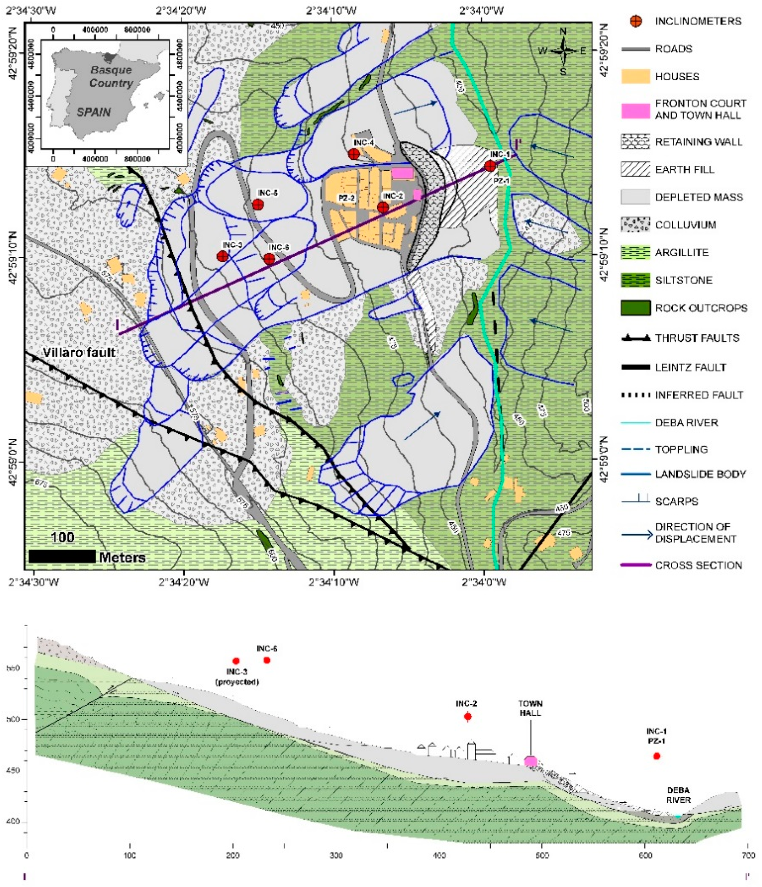
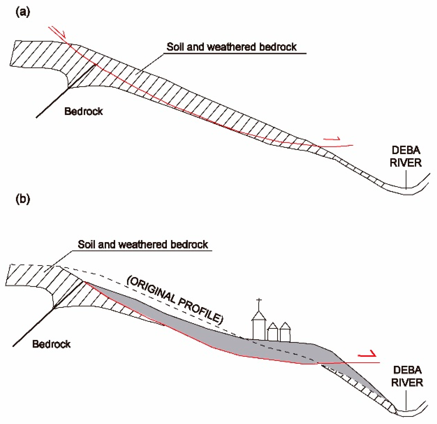
2. Leintz Gatzaga Landslide

2.1. Geological Context

The study area is located in the upper course of the Deba River, which flows through the province of Gipuzkoa (Basque Country, Spain). The relief of the Deba valley is quite abrupt and slope movements are frequent, mostly triggered by intense rainfall [16]. The region is tectonically complex, formed by arched shaped large-scale folds of Latter Jurassic and Early Cretaceous materials that belong to the Basque Arc [17]. Local geology and geomorphology is characterized by weathered cretaceous materials (argilites and siltstones) covered by quaternary colluvial deposits, high topographic relief and the presence of various faults (Figure 1).

We focus our work on a reactivated paleo-landslide whose complex motion has cause moderate to severe structural damage for centuries in Leintz Gatzaga medieval village [19], which has around 250 inhabitants and preserves an important historic heritage. The village settles on an east-facing slope that has an average gradient of 25%. On the slope, we distinguish different movements: the main landslide affecting the village, secondary lobes that develop within the main landslide body (with shallower slip surfaces) and smaller surfaces of rupture besides the main landslide. The width of the main landslide is 300 m and the length is 600 m. The main scarp of the landslide coincides with a thrust fault that puts in mechanical contact argillites and siltstones of the Urgonian and SupraUrogonian complex. The presence of this weak area, in conjunction with a thick weathered horizon and the erosive action of the Deba River at the toe of the slope, would have acted as main determinants of the paleo-movement that generated the current hill profile on which the village was funded in 1331, and after which the landslide was reactivated (Figure 2).

The lithostratigraphic column of the landslide is formed by four levels. The upper level is a low consistent clayey gravel earth fill which is constrained under the urbanized area. The second level is a high consistent colluvial deposit composed by low plasticity clay or clayey gravels, with large blocks of siltstone, argillites, and limestone which derive from rock falls of weathered Cretaceous bedrock from the upper cliff. Beneath it, there is a level of sandy gravels (composed entirely of siltstone), containing gypsum and pyrite veins. In some areas, the fines percentage increases to form sandy clays with gravels. This level has been defined as a “tectonic mylonite” [20], produced by ductile deformation of the bedrock due to shear strain accumulation of the inferred fault below Deba river, although it could just be an intense weathered product of the bedrock [18]. Finally, the substrate is formed by siltstones (Aptian–Albian age) that are in mechanical contact with calcareous argillites (Albian) by a thrust fault located at the landslide main scarp (northeast of Villaro fault). Several engineering works were performed in the last decades to alleviate landslide activity effects on Leintz Gatzaga buildings and infrastructures. In 1980, a drainage system was installed and a rock armour retaining wall was constructed at the foot of the slope (Figure 1). This solution had the objective of improving the bearing capacity of the terrain in that area, in order to build a fronton court and a new town hall, as the old one was dismantled due to structural failure caused by landslide activity. However, cracks appeared in the crown of the wall during the works and a strong rainfall period aggravated the problem in 1982. After that, the upper part of the wall was unloaded by excavating 1700 m³ of material. Between 1996 and 1998, micropiles were drilled in shallow foundations of a singular building and the fronton court. In 2009, the local council requested a geotechnical campaign to monitor landslide movements and establish the failure mechanism. Field observations indicate that the landslide is still moving, causing damage to several buildings, the fronton court area, and roads.

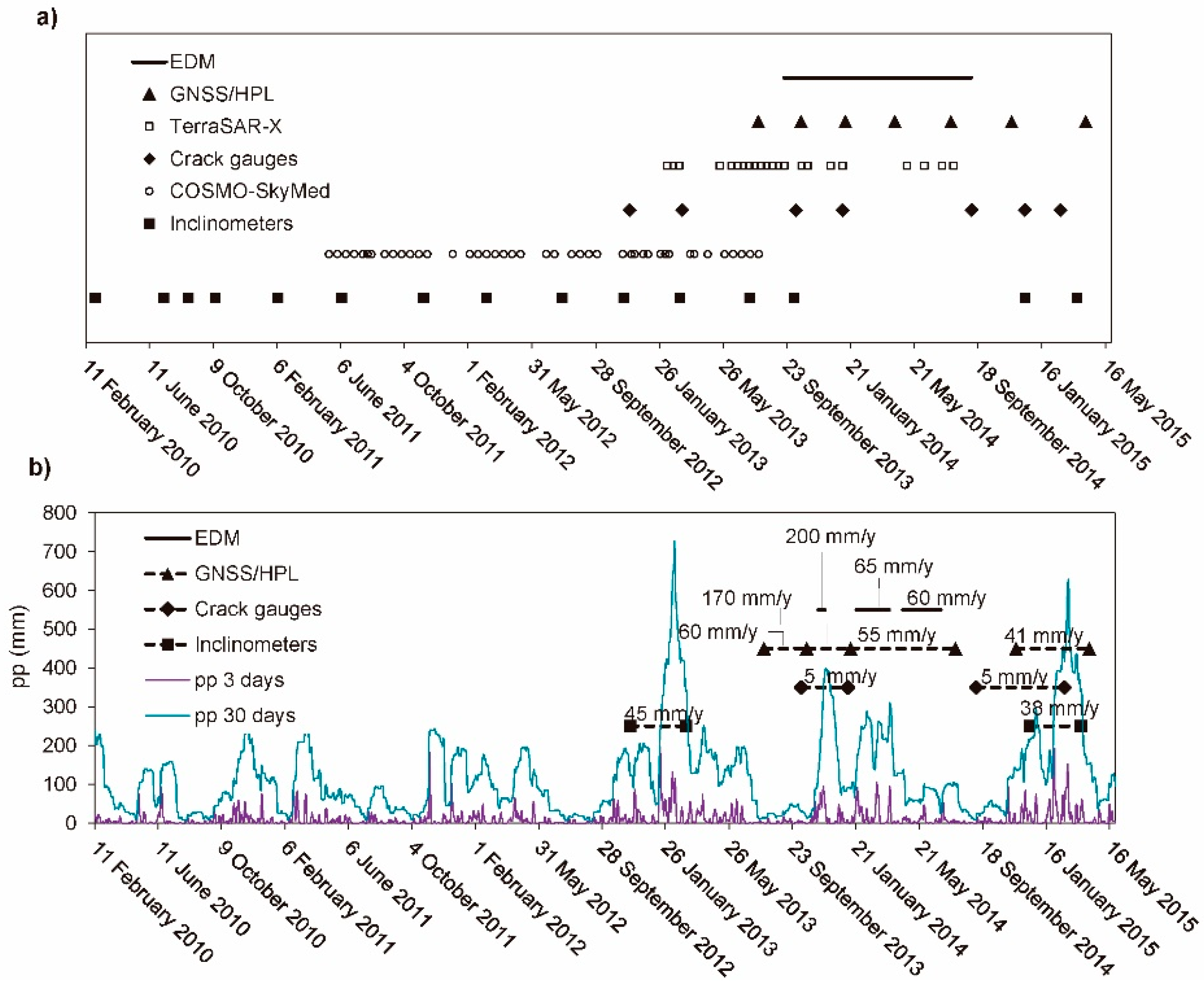
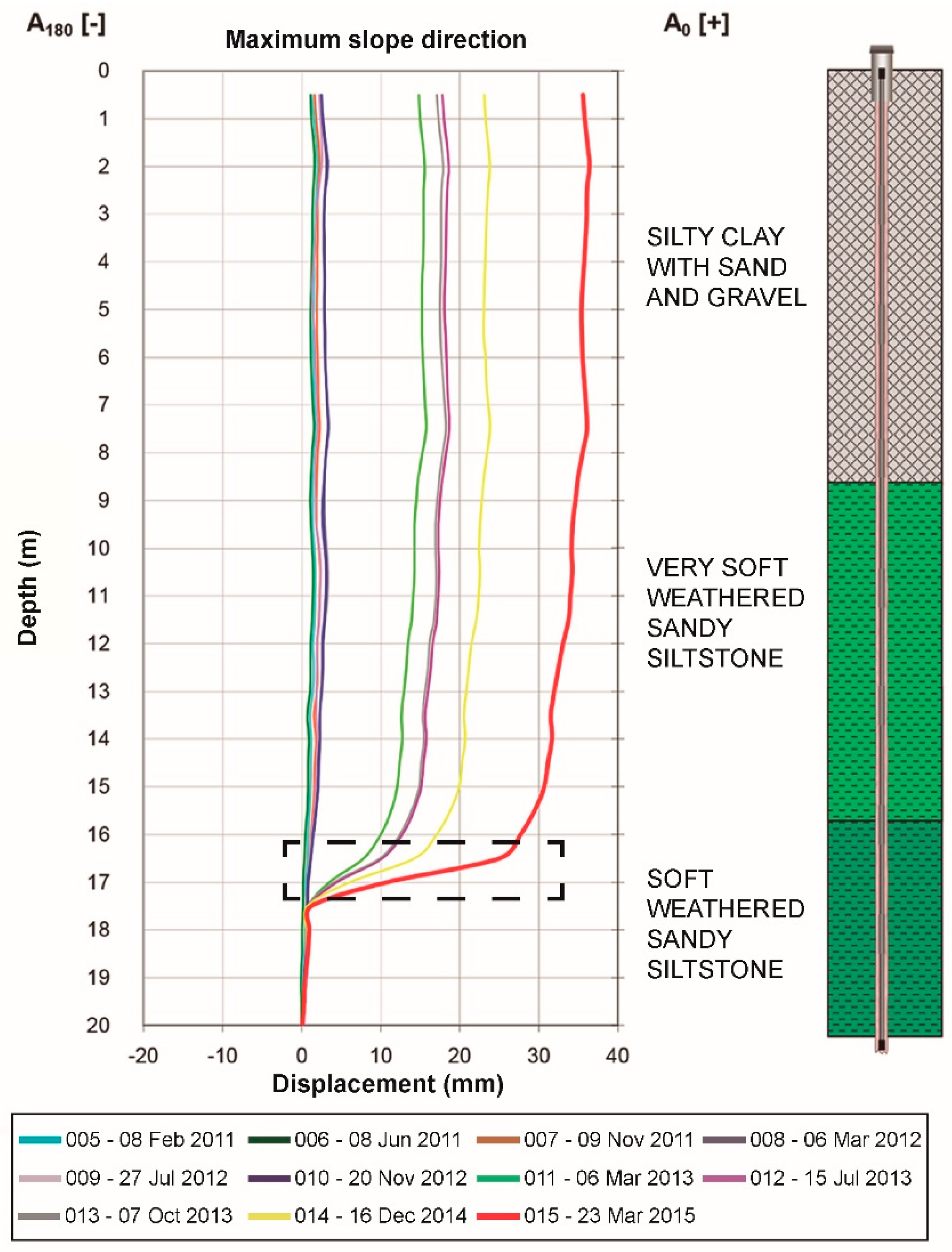
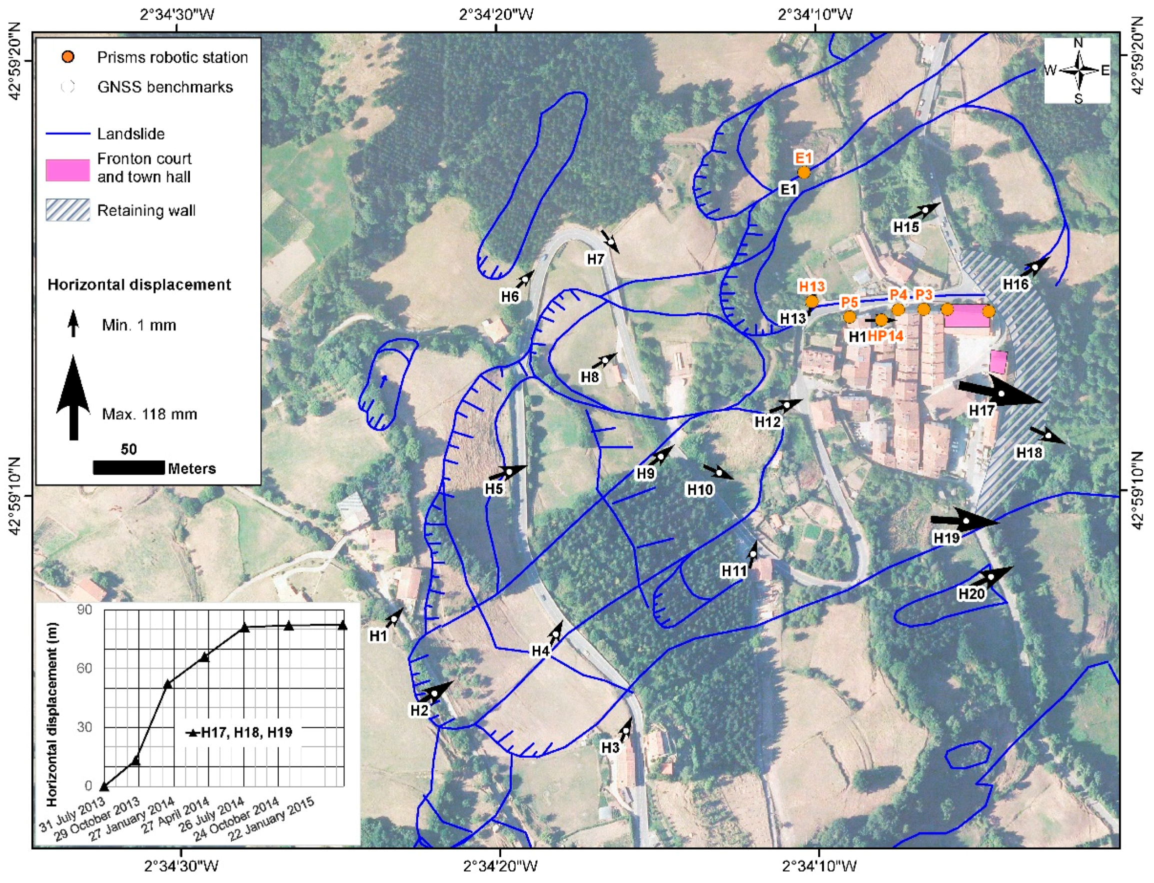
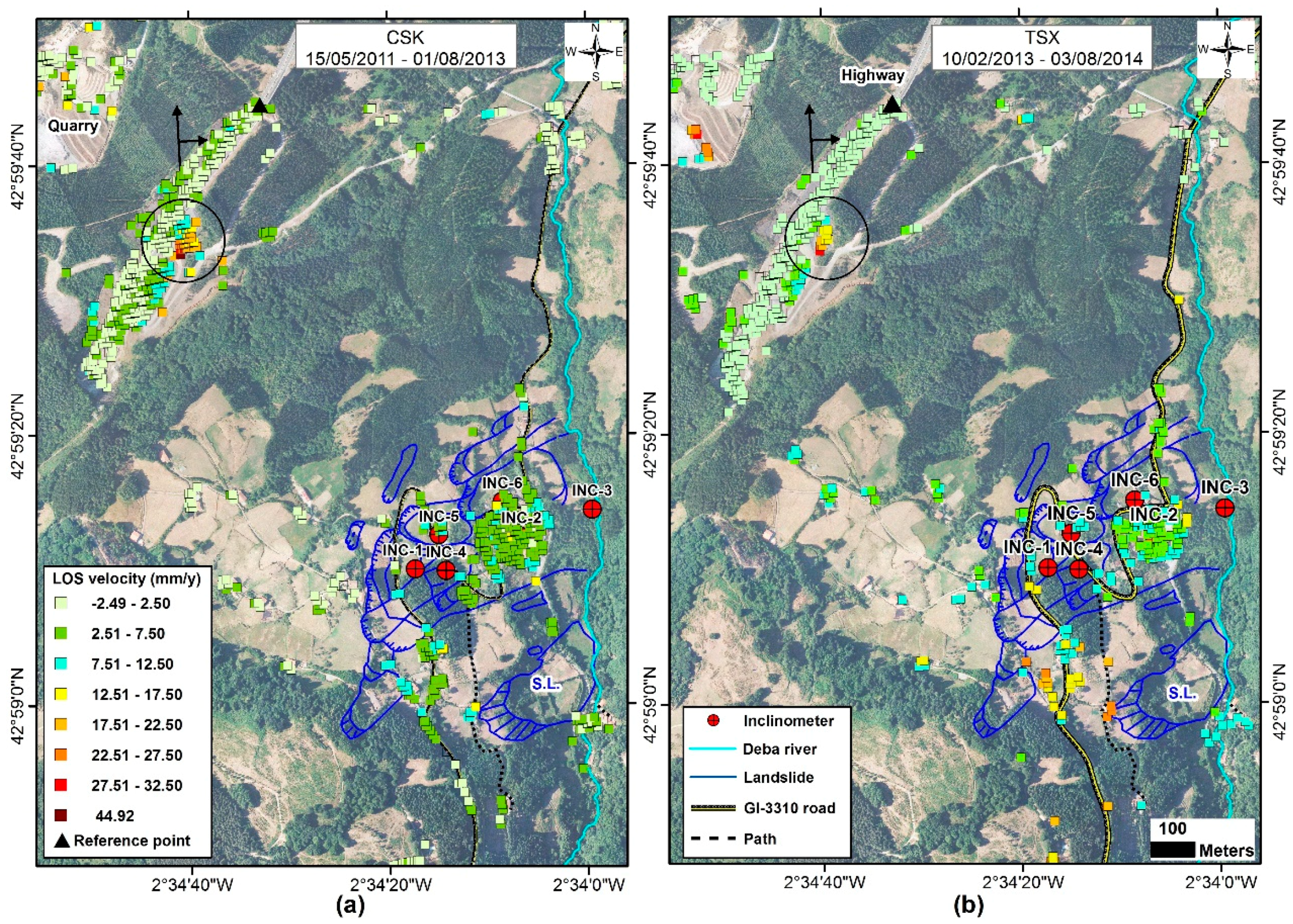
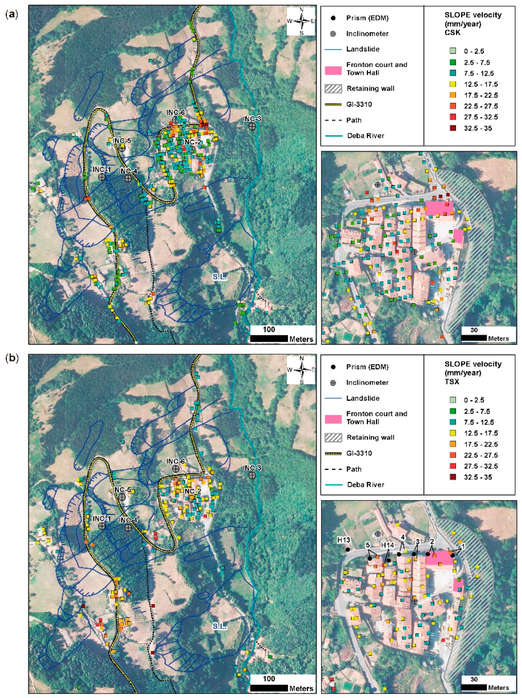
2.2. Monitoring Techniques Applied

Since 2010 different monitoring techniques have been used to measure the surface and in-depth displacements of Leintz Gatzaga landslide (Figure 3a). In this sub-section we will discuss the results obtained with the in situ monitoring techniques and their relation to accumulate precipitation data (Figure 3b). Remote sensing A-DInSAR techniques will be discussed in Section 3.3 of this manuscript.

Three inclinometers were installed in March 2010 (INC-1, INC-2, and INC-3), another one in October 2012 (INC-6) and two more in the beginning of 2013 (INC-4 and INC-5). The last reading available is from March 2015. Readings were performed manually every three months, although there is a gap of 14 months from October 2013 to December 2014. All inclinometers show displacement towards the maximum slope direction. For inclinometers INC-1, INC-2, and INC-3 core samples data are available, showing that the slip surface develops in weathered siltstone with soft to extremely soft consistence next to the contact with the bedrock. They detected the main slip surface at 16 m depth at the head of the landslide (INC-3), 28 m at the main body (INC-4), 23 m below the village (INC-2), and 13.5 m at the foot (INC-1). Inclinometers INC-5 and INC-6 detected shallower surface planes that develop within the margins of the main landslide body, at 12.5 m and 13.5 m, respectively. Shear deformation band concentrates within a narrow zone of about 1 m for all the inclinometers. A maximum accumulated displacement of 30 mm was measured in INC-3, which is located at the head of the landslide (Figure 4). Almost all of the movement was registered in two rainy periods from December 2012 to March 2013 and December 2014 to March 2015 with velocities around 40 mm/year.

Ten crack gauges were installed on the facades of the line of buildings located to the north of the village. Seven readings are available from December 2012 to February 2015. A maximum aperture of 4 mm was measured on one of the cracks of the fronton court. The opening of the cracks occurred in two periods, from October 2013 to January 2014 and from September 2014 to February 2015, while in the rest of the time the opening was negligible.

Six differential global navigation satellite system (GNSS) complemented with high precision levelling (HPL) campaigns were performed on 20 benchmarks covering the span time from July 2013 to November 2014 (Figure 5). GNSS precision in the horizontal plane is 3 mm ± 0.5 ppm and HPL has a typical deviation of 0.3 mm in 1 km of double levelling. The direction of the movement is towards the maximum slope direction. Maximum displacements were detected in the village area close to the retaining wall, up to 118 mm in the horizontal plane. Displacements measured on the landslide do not follow the same pattern. However the benchmarks with maximum displacement (H17, H18, and H19) do all register movement since the first reading. We calculated the arithmetic mean of the horizontal displacement measured in each of those benchmarks (inset Figure 5), from which we can extract a mean velocity of 60 mm/year from the end of July to middle October 2013, followed by an increment of velocity (170 mm/year) until January 2014 and followed by a decrease of velocity (55 mm/year) until July 2014. An additional measurement was made in April 2015 just on these three benchmarks.

Continuous recording of the displacements of seven prism reflectors were performed automatically during 352 days, from September 2013 to September 2014, with an electronic distance measurement (EDM). The robotic station featured a communication system to obtain the data remotely in real time. Five prism reflectors (P1–P5 in Figure 5) were placed on the facades of the line of buildings located to the north of the village and a two more housed inside H13 and H14 benchmarks (Figure 5). The displacement pattern is similar for all of them, with the exception of H13. A mean velocity of 200 mm/year was recorded between 11 November 2013 and 23 November 2013 (Figure 3). After that, there was not significant movement until the period between 17 January 2014 to 25 March 2014, with mean velocity of 65 mm/year. In April 2015, there is a jump in the time series, due to subtraction of a reference prism, which has been corrected for later comparison with interferometric displacement data in the Section 3.3.4 of this manuscript. From 20 April 2014 to 1 July 2014, a mean velocity of 60 mm/year was measured.

Additionally, two vibrating wire piezometers were installed in 2010 at the toe of the landslide (PZ-1) and in the village (PZ-2) to measure pore pressures at three different depths positions. Until 2014 readings were made manually every three months. The large discontinuity of readings masked short- and medium-term fluctuations. In 2014, datalogger sensors were installed in the piezometers performing readings two times a day. The piezometric level at PZ-2 was located at 3 m depth from the surface and reacts immediately to precipitation, ranging between 2.5 m and 3.66 m.

2.3. Landslide Classification and Activity

The variety and complexity of unstable slope phenomena brings the need for a system of classification to characterize the landslide behavior, being crucial to define the state of activity. The current profile of the slope is the result of a mass movement of predominantly fine material (clayey soil) that occurred before the village was settled. The landslide style is characterize by a main body and secondary lobes of displaced masses formed by repeated movements of the same type. Urban damage, geomorphological feature inspection, and ground monitoring data show that the landslide was active in the studied period. Therefore, we classify the landslide as a reactivated multiple earth slide according to Cruden and Varnes classification [21]. Also, according to the measured displacements, we distinguish two patterns that are directly related to accumulated rainfall infiltration (Figure 3b). The first one corresponds to an extremely slow landslide velocity and the second to a very slow velocity one. The depleted volume of the Leintz Gatzaga landslide is of about 2.6 × 10⁶ m³, which corresponds to a very large magnitude landslide according to Fell classification [22].

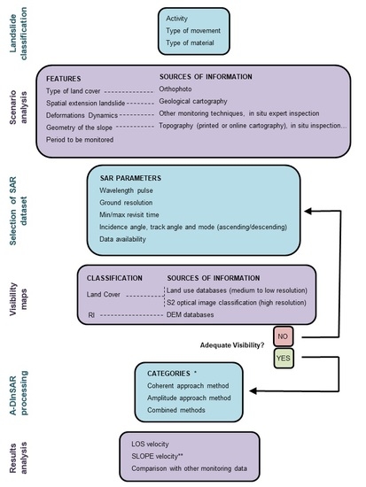
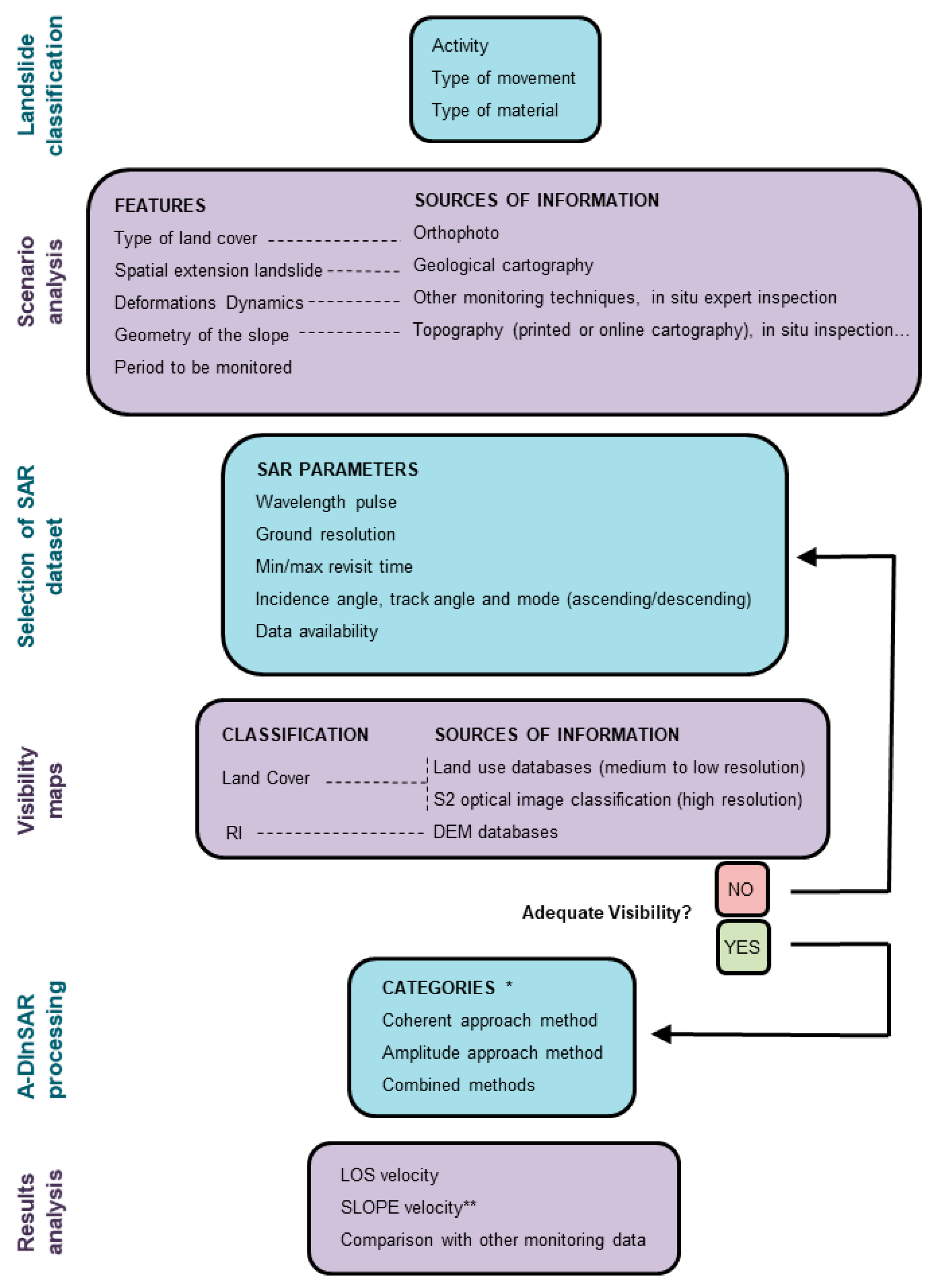
3. Practical Guidelines for Complex Monitoring of Slow Moving Landslides

Our main objective is to propose a procedure which can serve as a practical guidelines of complex monitoring of site scale slow moving landslides including remote sensing A-DInSAR techniques, to be used by civil protection agencies, local authorities, and private building companies. A summary of the procedure is outlined in the flow chart shown in Figure 6. Further description of the procedure is detailed in the following sub-sections. Section 3.1 includes the scenario analysis of the studied area and the SAR dataset selection. Section 3.2 describes the classification of the land cover data (from high resolution Sentinel 2 optical data) and geometrical visibility, which will be used to create the visibility maps. Finally, Section 3.3 includes the A-DInSAR processing with the selected category, the assessment of high resolution qualitative visibility map production, and analysis of the monitoring results.

3.1. SAR Dataset Selection

The selection of the appropriate SAR dataset suitable for studying a specific area is crucial. The objective is to detect as much reliable targets to be measurable through time in order to obtain dense spatial coverage of surface displacements. This depends on several factors related to both the scene characteristics (such as land coverage, the extent of the area of interest, deformation dynamics) and the sensor specifications (such as carrier frequency, image resolution, and revisiting time). For the particular case of landslide processes, another determinant factor to take into account is the geometry of the slope where the instability occurs. The last—but not least—consideration is data availability, especially when archived images are needed for historical analysis. The constrains and limitations when using A-DInSAR techniques to monitor landslides have been discussed in literature [11,12,13,24] and several authors have proposed “pre-processing” guidance and methodologies to study the suitability and reliability of applying these techniques for particular landslides [25,26,27,28]. In this sub-section, we will discuss the considerations to select an adequate dataset for the studied area and asses its visibility taking into account the geometrical parameters of the SAR images, the type of land cover, and geometrical distortions.

3.1.1. Particular Characteristics of the Landslide Scene

In order to select an appropriate SAR dataset, we take into account the principal characteristics of the scene where the landslide phenomena takes place:

• Type of land cover: in our test-case the area of interest is characterized by both small patches of man-made structures (the village, sparse construction, and roads), which are usually coherent, and vegetated zones (pastures and forest), which instead are generally less coherent.
• Spatial extent of the phenomena: landslide extent is in the order of 300 × 600 m².
• Deformation dynamics: according to in situ monitoring data, the expected velocity of the landslide varies between extremely slow velocity and very slow velocity according to Cruden and Varnes classification [21], depending on rainfall infiltration.
• Geometry of the slope: the landslide is located on a slope that faces east, with an average inclination of 25%.
• Period to be monitored: from early 2010 to middle 2015.

The type of land cover of the scene and the wavelength of the satellite radar sensor will determine the amount of CTs at which displacements can be measured by A-DinSAR techniques. To consider a portion of the terrain as a CT, the backscattering properties of that area should remain stable between the dates of SAR image acquisitions. The latter occurs in bare surfaces such as rock outcrops and urbanized areas, whereas the contrary takes place in surfaces that rapidly vary their backscattering properties due to ambient factors, such as plant growth and wind, which produces the effect known as temporal decorrelation [6]. Typical values of radar sensor wavelength pulses are 3.1 cm for X-band, 5.6 cm for C-band, and 23.6 cm for L-band. The greater the wavelength, the greater the penetration capability in vegetated areas, and the lower the sensitivity of the differential phase to deformation [29].

For local scale studies as the one at hand, an orthophoto and local cartography can be enough to discern at least between vegetated and urbanized areas, giving a general overview that will help in choosing the most suitable radar frequency band. Figure 7a shows the combination of a 5 m resolution orthophoto provided by the Spanish National Geographic Institute (IGN) [30] and cadastral cartography provided by the regional database of Gipuzkoa council [31]. Vegetated zones constitute nearly the 90% of the analyzed area. Dark green corresponds to conifer forest and scrubland (labelled by F) and very pale green to grasslands (G), which are mainly destined for grazing. The village occupies an extent of 0.02 km², the average area of sparse constructions is 300 m² and regional roads are 8 m wide. There are also unpaved trails 3 m wide crossing grazing areas, forest, and along the riverside. With this brief information of the land cover of Leintz Gatzaga study area, we maintain that the most suitable choice is X-band. The fine resolution of the satellites that operate in this band will be able to detect the small coherent patches that are well distributed in the studied area [32]. Moreover, the short temporal sampling of X-band satellites can be crucial when the deformation phenomenon to be monitored is fast or shows an important non-linear behavior. Nevertheless, the use of A-DInSAR data is limited to landslides, ranging from extremely slow to very slow phenomena, according to the velocity classification of Cruden and Varnes [21], due to phase measurement ambiguity [33]. Additionally, shorter wavelength implies a better sensitivity of the differential phase to displacement, although at the same time, the interferograms are more affected by temporal and volumetric decorrelation, thus causing strong decorrelation in all types of vegetated areas. These effects will limit the sampling density of the surface monitoring of the studied area, which is one of the disadvantages of A-DInSAR techniques, while still being a drastic improvement over classical monitoring methods.

We discarded C-band data from Envisat and ERS satellites (ESA) to perform a historical analysis of the landslide due to their low spatial resolution, which is 4 m in azimuth and 20 m in ground range if working at full resolution and much less if applying a multilook with a SBAS coherence-based techniques. However, other techniques that combine permanent scatterers and distributed scatterers—such as SqueeSAR [34]—could improve the results of C band data in areas like Leintz Gatzaga. Just a few CTs would be detected in large areas where phase quality is preserved along time (village) and none in area covered by smaller man-made structures (sparse constructions and roads). However, other satellite products which operate in C-band with enhanced spatial resolution, such as RADARSAT-2 (Canadian Space Agency, CSA) or recently launched Sentinel-1 (ESA) satellite mission, could be appropriate for this scenario in further studies. Sentinel-1 is a small baselines constellation with a low revisit time (six days in constellation, 12 days per satellite) which ensures low temporal baselines between acquisitions. ALOS-1 PALSAR data (Japanese Spatial Agency, JAXA), which have a spatial resolution of about 10 m, would be also suitable for this application because the L-band is characterized by a greater foliage penetration capability, thus extending the coverage to landslides in relatively vegetated areas [35]. However, the longer revisiting time of this satellite (46 days) reduces the quality of both the displacement velocity and the displacement time series [36]. Indeed, only a few images with large baselines were available in the archive for use in this study, which are not enough to obtain reliable results. A significant improvement for L-band sensors is ALOS-2 satellite, which was launched in mid-2014 and has revisiting cycle of 14 days.

3.1.2. Selected SAR Datasets Parameters

Second generation satellites [32] working at X-band, such as COSMO-SkyMed (Italian Space Agency, ASI) or TerraSAR-X (German Aerospace Centre, DLR), provide SAR products mainly on demand. However, sometimes historical data are available from previous planning. COSMO-SkyMed (CSK) is a four-spacecraft constellation whose single satellite has a 16 days repeat cycle; the final revisit time can be significantly shorter depending on the number of active satellites and their configuration. A set of 43 ascending Stripmap HIMAGE mode SAR images was available in the CSK archive, covering the period from 15 May 2011 to 1 August 2013. The time interval overlaps inclinometric and crack gauge data (Figure 3a) allowing us to compare A-DInSAR data to ground truth one. The minimum time interval between subsequent images of the available CSK dataset is eight days, while the maximum is 48 days. We also acquired, by request, 22 High Resolution Spotlight TerraSAR-X (TSX) images covering the period from 10 February 2013 to 3 August 2014, which overlaps inclinometric, crack gauge, GNSS/HPL, and EDM data (Figure 3a). The repeat cycle of the TSX satellite is 11 days and the maximum interval between subsequent images of the available dataset is 121 days. Spotlight mode has the advantage of having a fine ground projected resolution (0.9 × 1.6 m), although in our case ground resolution is lowered due to the SBAS approach that uses multilook (ML). To obtain a ground resolution of 10 × 10 m, the ML factor used for the TSX Spotlight mode (13 × 7) is greater than the one use for the CSK Stripmap mode (5 × 5). The fact that more pixels are averaged allows reducing the coherence threshold of the TSX interferograms for the same phase standard deviation. Datasets acquisition parameters are summarized in

Table 1. Acquisition parameters of the selected datasets.

Sensor	CSK	TSX
Number of images	43	22
Acquisition orbit	Ascending	Ascending
Acquisition mode	Stripmap HIMAGE	High Resolution Spotlight (HS)
Polarization	HH	HH
Temporal interval	15 May 2011 to 1 August 2013	10 February 2013 to 3 August 2014
Minimum revisit time (days)	7	11
Maximum revisit time (days)	48	121
Incidence angle (°)	27	35
Tracking angle (°)	348	350
Ground projected resolution (Azimut × Range)	2.2 m × 2.2 m	0.9 m × 1.6 m
Multilook factor applied (Azimuth × Range)	5 × 5	13 × 7
Ground resolution with ML	≈10 m × 10 m	≈10 m × 10 m

.

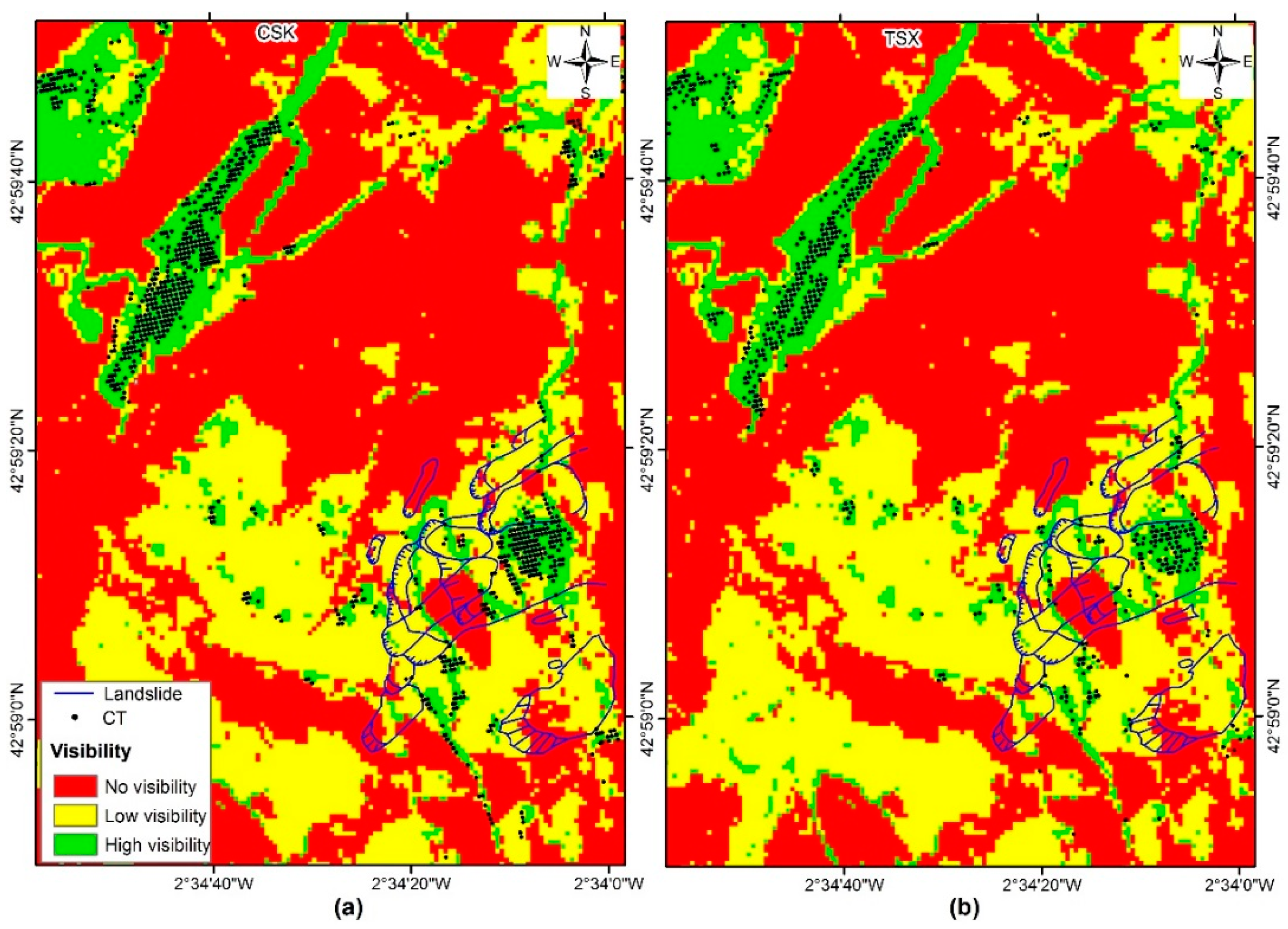
3.2. Visibility Analysis

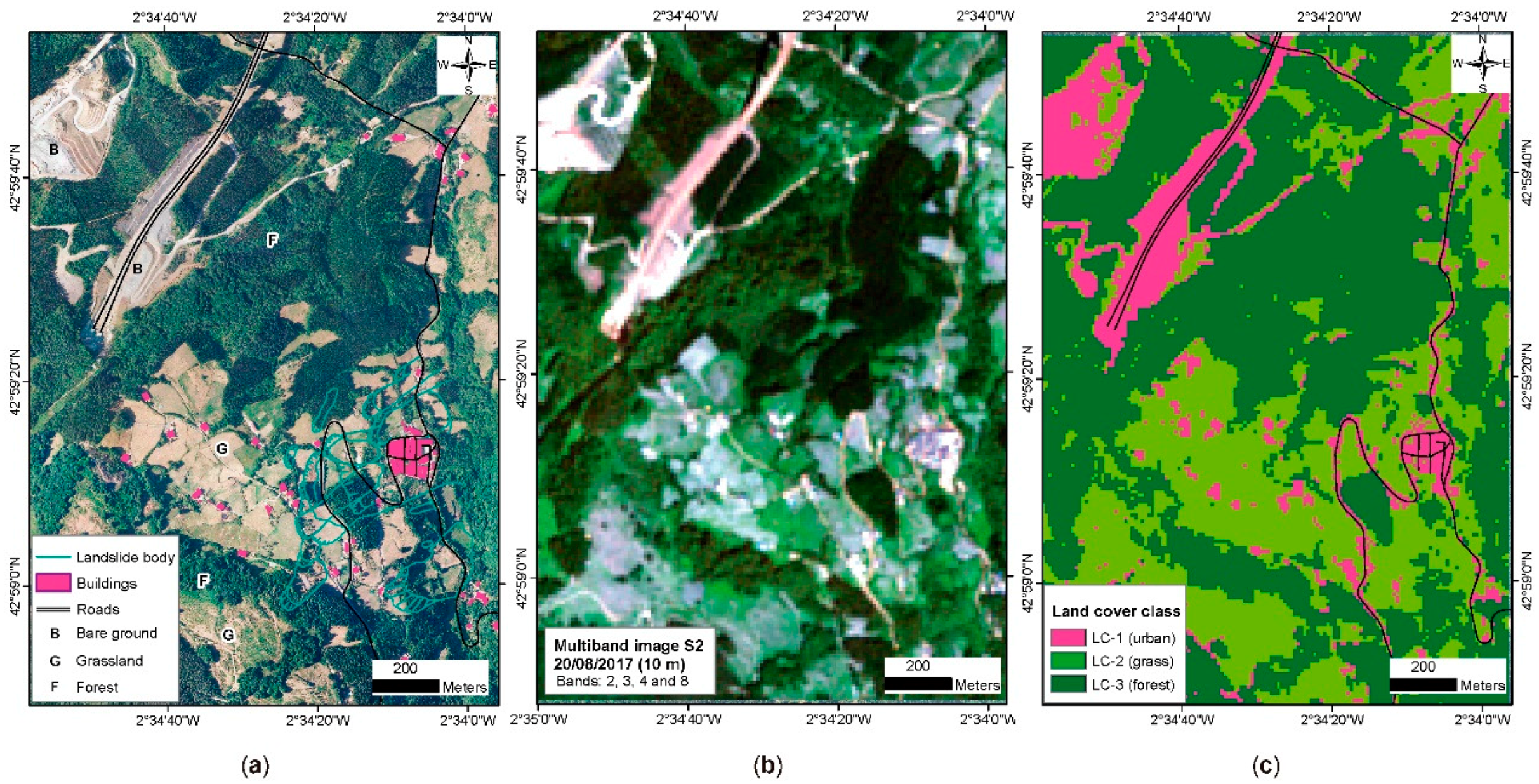
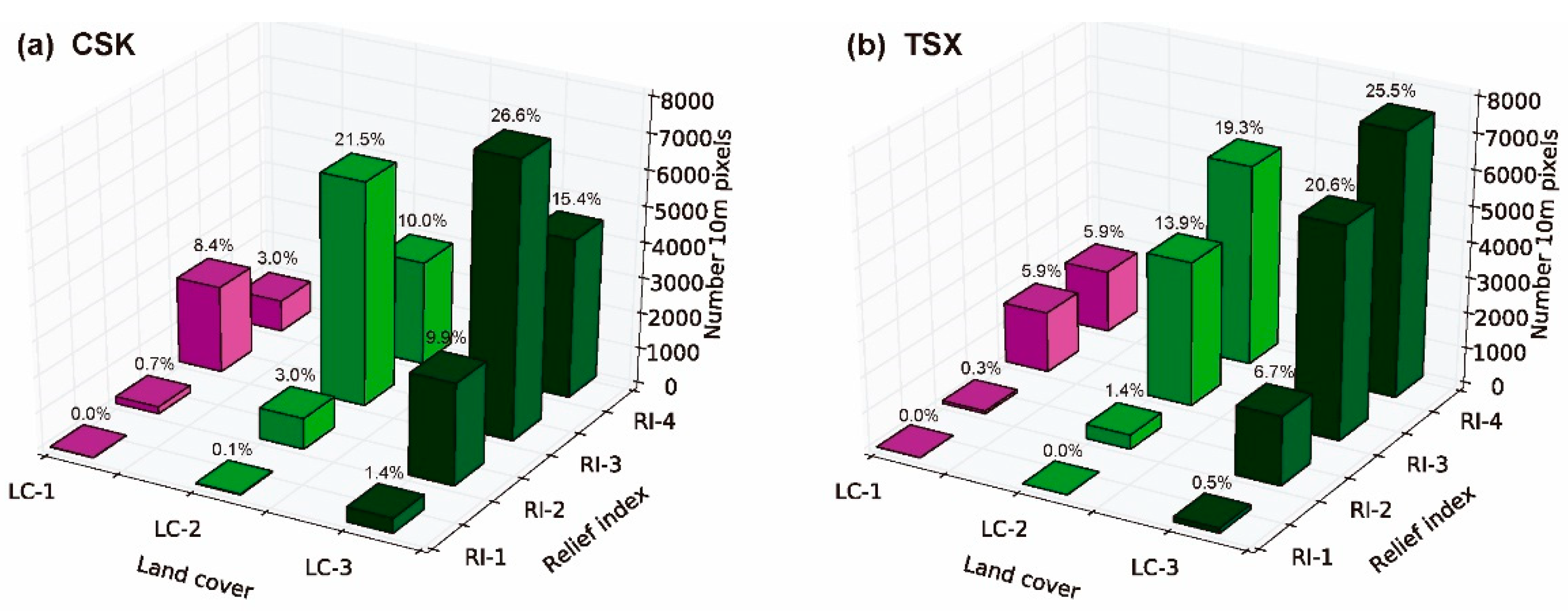
3.2.1. Land Cover Classification

International and regional land cover databases are freely available as cartographic products. Some examples are the Coordination of Information on the Environment project from the European Environmental Agency (CORINE) or the Spanish land use information system (SIOSE) from the Spanish National Plan for Territory Observation (PNOT). However, these databases have a medium-low spatial resolution (the minimum mapping unit of SIOSE for urban areas is one hectare and for natural and agricultural areas is two hectares), which is not useful to site scale case studies as the one in hand.

High resolution land cover information, in order to assess the expected CTs density in small-scale areas of interest, can be achieved with high resolution optical data. In that respect, we exploit optical images acquired by Sentinel-2 (S2) ESA mission, that comprises twin satellites flying in the same orbit but phased at 180°, with a revisit frequency of five days at the Equator. Sentinel-2A satellite was launched on 23 June 2015 and Sentinel-2B on 07 March 2017. They carry an optical instrument payload that samples 13 spectral bands: four bands at 10 m, six bands at 20 m, and three bands at 60 m spatial resolution, ideal for land classification purposes [37].

Image classification refers to the task of extracting information classes from a multiband raster image, resulting on thematic maps such as land cover types. The two most common approaches are supervised and unsupervised image classification techniques, depending on the interaction between the analyst and the computer during classification [38]. The former uses the spectral signatures obtained from training samples to classify an image. The latter finds spectral classes without the analyst’s intervention. Among the various algorithms geared toward supervised classification, one of the most common used is maximum likelihood classification. We performed land cover classifications in two S2 images acquired at 22 April 2017 and 20 August 2017. The selection criteria was to have a low cloud shadow percentage (0.16 and 0.15 respectively) and to belong to different seasons. The former corresponds to the end of the rainy season (84.4 mm of precipitation accumulated in the previous 30 days) and the latter to summer that is typically dry (16.1 mm of precipitation accumulated in the previous 30 days). We tested different band combinations and resolutions of 10 and 20 m. In order to gain a relative evaluation between the classifications, we calculated statistics using the kappa coefficient of agreement [39]. The first step was to identify the main classes of land cover according to the area of interest characteristics, the preservation of coherence among time and the X radar wavelength. We distinguish three classes of pixels:

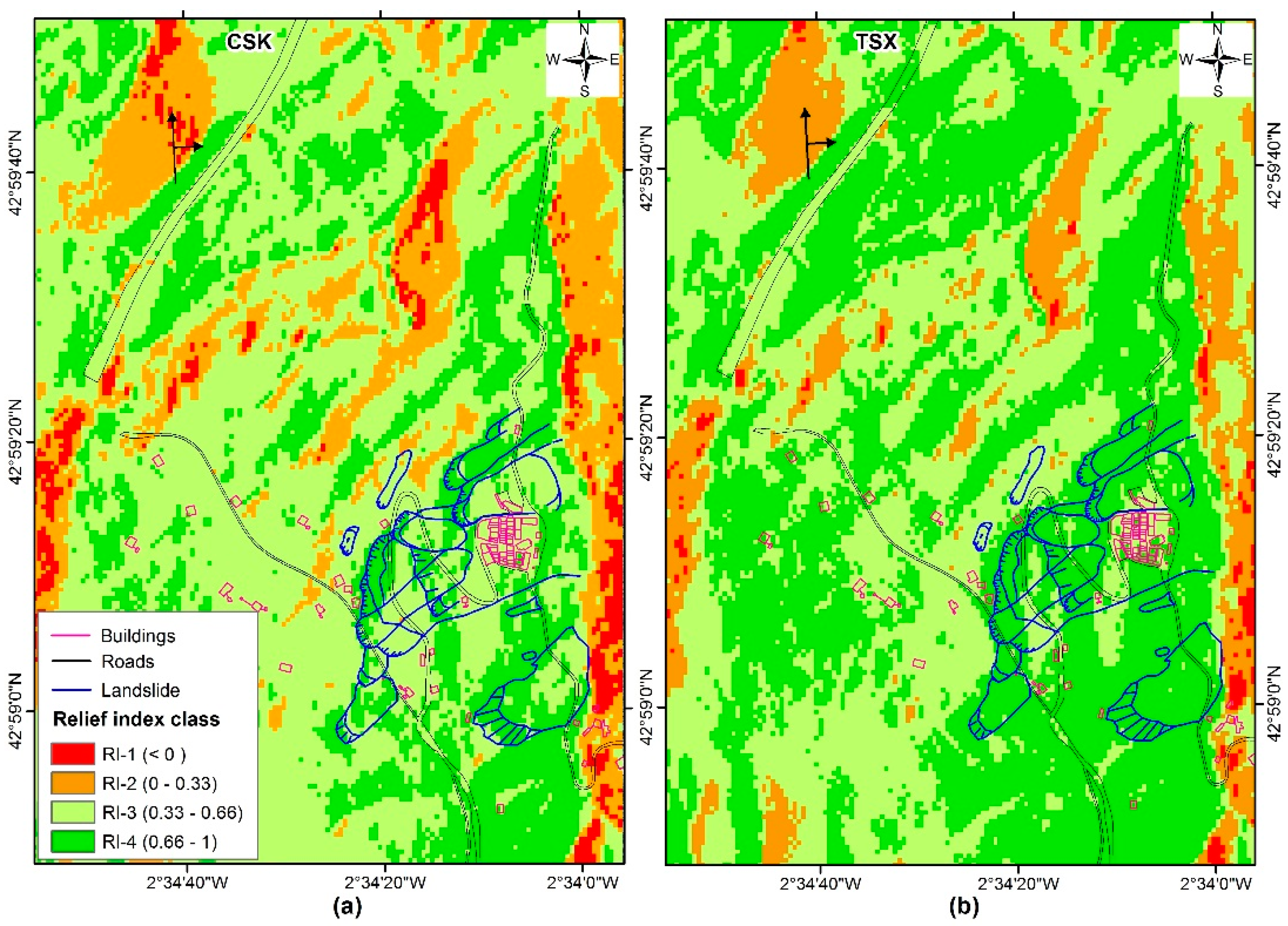
• LC-1: Urban (buildings, roads and bare ground). Coherence is expected to be very well preserved through time.
• LC-2: Grasslands. Coherence is expected to be poorly preserved.
• LC-3: Forest. Coherence is expected to be completely lost.

The second step was to combine spectral bands sampled by S2 at 10 m and 20 m spatial resolution to create the multiband images of the area of interest (that has an extent of 2020 × 1440 m). The spectral bands used for each combination can be found in the third column of

Table 2. Kappa coefficients of 14 land cover classifications obtained from multiband images. The distribution, in terms of percentage, of the land cover (LC) classes on the studied scene (extent of 2020 × 1440 m) is also shown. The last columns show the percentage of detected coherent targets (CT) of CSK and TSX datasets for each LC class. Note that the number of pixels of the whole scene is 29,088 for the 10 m resolution images and 7373 for the 20 m resolution ones.

				LC Class Distribution (%) of the Studied Scene			Detected CTs (%) for Each LC Class
							CSK (926 CTs)			TSX (658 CTs)
Cell Resolution (m)	S2 Image	Bands Combination	Kappa Coefficient	LC-1	LC-2	LC-3	LC-1	LC-2	LC-3	LC-1	LC-2	LC-3
10 (29,088 pixels)	22 August 2017	3,4,2	0.69	16.2	33.6	50.2	85.1	12.1	2.8	88.8	7.8	3.5
		2,3,4,8	0.785	16.6	30.8	52.6	85.2	11.4	3.3	89.7	6.8	3.5
	20 August 2017	3,4,2	0.807	12.6	35.9	51.5	79.6	18.6	1.8	82.8	14.1	3
		2,3,4,8	0.813	12.1	34.6	53.3	79.9	17.5	2.6	86.6	10.9	2.4
20 (7373 pixels)	22 April 2017	3,4,2	0.63	16.2	34.4	49.4	83.9	13.3	2.8	86.6	10.6	2.7
		2,3,4,8A	0.694	18.9	28.9	52.2	87.7	8.7	3.6	90.1	7.3	2.6
		5,4,2	0.652	16.8	33.5	49.7	84.7	12.3	3	89.1	8.1	2.9
		7,4,2	0.666	17.6	29.4	53	84.7	10.7	4.6	88	8.1	4
		2,3,4,5,6,7,8A,11,12	0.75	21	28.5	50.5	95.5	3.3	1.2	94.4	4.1	1.5
	20 August 2017	3,4,2	0.697	13.5	35.6	50.9	81.4	16.4	2.2	87.8	10.6	1.5
		2,3,4,8A	0.688	12.9	36	51.1	80.1	17.6	2.3	86.5	12.3	1.2
		5,4,2	0.705	13.6	36.1	50.3	79.8	18	2.2	85.4	11.9	2.7
		7,4,2	0.681	12.8	35.9	51.3	78	20	2	85.6	13.4	1.1
		2,3,4,5,6,7,8A,11,12	0.754	17.8	28.8	53.4	90.9	5.9	3.1	93	4.6	2.4
			Ave.	15.6	33.0	51.4	84.0	13.3	2.7	88.2	9.3	2.5
			Max.	21.0	36.1	53.4	95.5	20.0	4.6	94.4	14.1	4.0
			Min.	12.1	28.5	49.4	78.0	3.3	1.2	82.8	4.1	1.1

. Then we created training samples in order to identify classes. We ensured that training samples were representative for the area using a 0.25 cell resolution orthophoto, Google Earth map service system, and in situ evaluation during field campaigns. The percentage of training samples area with respect to the whole study area clip is 20.6%. We generated 14 land cover classifications (Table 2), one for each multiband image, using a maximum likelihood algorithm. The evaluation of the statistical significance of the difference in accuracy between two thematic maps derived from remotely sensed data has often been based on the comparison of the kappa coefficient calculated for each map [40]. The kappa coefficient of agreement for a thematic map is based on the comparison of the predicted and actual class labels for each case in the testing set and may be calculated from [39]

$$\mathrm{K}=\frac{{\mathrm{P}}_0-{\mathrm{P}}_{\mathrm{C}}}{1-{\mathrm{P}}_{\mathrm{C}}},$$

(1)

where P₀ is the proportion of cases in agreement (i.e., correctly allocated) and P_C is the proportion of agreement that is expected by chance. To compute these proportions, we calculated the error matrix (or confusion matrix) of each classification, which are tables that show correspondence between the predicted class (classification results) and the actual class (ground truth). Error matrices are available in the Supplementary Material (Table S1). The kappa coefficients and the percentage occupied by each land cover class is shown in Table 2. According to the classification results, the area of interest is mostly covered by LC-3 class (forest) with mean percentage of 51.4%, followed by LC-2 (grass) with mean percentage of 33% and LC-1 (urban) with mean percentage 15.6%. LC-3 is the class whose percentage varies the least among different classifications and LC-1 the one that varies the most. In general, the classifications obtained from the S2 image of April detect more amount of LC-1. The best kappa coefficient is the one that corresponds to the classification obtained from S2 image of 20 August 2017 with a resolution of 10 m and two-, three-, four-, and eight-band combination (Figure 7b,c).

3.2.2. Geometrical Distortion (Relief Index) Classification

The side look acquisition mode of the SAR satellites antenna produces geometrical distortions of the terrain area that is imaged in each SAR resolution cell when the topography is not flat [41]. This complicates landslide monitoring with A-DInSAR techniques, as they typically develop along slopes, and careful analysis should be made in order to select the best available acquisition configuration. In general terms, the descending and ascending geometries are favorable, respectively, for west and east facing slopes [25] and landslides that present an orientation parallel to the satellite orbit (quasi polar) will have motion orthogonal to the LOS and thus be undetectable. In a SAR image, the features of the scene are projected along the radar line of sight (LOS, also known as the “slant-range”); or, in other words, ordered depending upon its distance from the satellite along its side-looking direction. Consequently, the terrain slopes facing the radar appear compressed in the image, known as foreshortening effect, and if the inclination of the slope exceeds the incidence angle, the scatters are imaged in reverse order and superimposed on the contribution coming from other areas, causing the layover effect [6,42]. On the other hand, scatters located on the opposite side can be affected by two distortions; if terrain slope is equal to the radar incidence angle the cell dimension becomes very large and details are lost and if the terrain slope exceeds the radar incidence angle the resolution cells cannot be imaged as they are in shadow. The inclination and orientation of slopes can be easily derived from a digital elevation model (DEM) using a geographic information system (GIS). National and regional cartographic open databases in Spain, such as the National Geographic Institute (IGN), provide a wide range of topographic data and DEMs with resolutions up to 2 m. The topographic information can eventually be combined with the orbit parameters of the SAR images datasets to obtain a geometrical visibility map [13,25,43,44]. We use the relief index (RI) [26] in order to check if coherent targets will be visible in the Leintz Gatzaga study area using the CSK and TSX datasets. RI equation [26] is defined as the ratio between the slant range and the ground range, taking into account the acquisition geometry of the radar and the orientation (aspect model) and inclination (slope model) of the terrain

$$\mathrm{RI}=-\sin \left\{[\left(\mathrm{S}\times \sin \left(\mathrm{A}\right)\right]-\sin \left(\mathrm{i}\right)\right\},$$

(2)

where S is the slope, A is the corrected aspect with respect to the track angle of ascending or descending orbit mode, and i is the incidence or ‘off–nadir’ angle of the satellite antenna. Values of the RI range from −1 (layover or shadow effects) to +1 (slope with very good geometrical visibility). We define four classes according to [45]. For the first class (RI-1), no CTs can be detected due to geometrical distortions such as layover and shadow effects for negative values and foreshortening effect for RI values very close to zero. The second class (RI-2) comprises values between 0 and 0.33 and indicates that the slope geometry is not favorable for the satellite LOS geometry; therefore, it is expected to retrieve a lower number of CTs. RI-3 comprises values between 0.33 and 0.66 and indicates flat areas or slopes with an acceptable geometry with respect to the satellite LOS. In general, when the value of RI is greater than 0.3, the slope is well-oriented and the main factor that influences the CTs distribution is land use [26]. Finally, RI-4 (values from 0.66 to +1) stands for areas where the slope direction is approximately parallel to the satellite LOS direction and therefore are the most suitable areas to detect CTs.

To calculate the slope and aspect necessary to obtain the geometrical visibility maps, we used a 5 m resolution DEM provided by IGN [46], which we resampled to 10 m and 20 m. As for the case of land cover classifications, the 10 m resolution cell scene gives 29,088 pixels and the 20 m resolution cell scene 7373 pixels. The acquisition characteristics of the two SAR datasets are included in Table 1. Figure 8 shows the 10 m resolution RI maps of the CSK and TSX datasets of Leintz Gatzaga study area. For both datasets, RI maps indicate that most of the landslide extent has good to very good geometrical visibility. Note that the opposite slope of the valley that faces west shows low RI values. In the case of CSK dataset geometry, the most common class is RI-3, both for the whole clip and landslide extent, while for the TSX is RI-4. CSK dataset has a worse geometrical visibility because of its smaller incidence angle that induces higher topographic effects [14]. The distribution of each class of the four RI maps is included in

Table 3. Distribution, in terms of percentage, of the RI classes on the studied scene (extent of 2020 × 1440 m). Bottom rows show the percentage of detected coherent targets (CT) of CSK and TSX datasets for each RI class.

	RI Class Distribution (%) of the Studied Scene
Cell resolution (m)	CSK geometry				TSX geometry
	RI-1	RI-2	RI-3	RI-4	RI-1	RI-2	RI-3	RI-4
10	1.5	13.6	56.5	28.4	0.5	8.4	40.3	50.8
20	1.6	13.5	56.4	28.2	0.6	8.7	40	50.7
	Detected CT (%) for each RI class
	CSK dataset (926 CT)				TSX dataset (658 CT)
	RI-1	RI-2	RI-3	RI-4	RI-1	RI-2	RI-3	RI-4
10	0	1.1	74.9	24	0	0.3	54.9	44.8
20	0	0.6	76.3	23	0	0.2	52.1	47.4

in terms of percentage.

3.2.3. Land Cover and RI Classes’ Distribution

If we combine land cover and relief visibility data we obtain the relative distribution of LC and RI classes of the cells or pixels that conform the studied scene. Histograms of Figure 9 show the LC and RI distribution of the 29,088 pixels (10 m resolution) of the multiband image with the best kappa coefficient (two-, three-, four-, eight-spectral band combination, date 20 August 2017, cell resolution 10 m, Table 2) and the relief classifications for the CSK and TSX geometries (Table 3). The shape of the graphs are the same for any LC classification and cell resolution, although the total number of pixels for each class varies. For all the computed LC classifications, the scene is mostly composed by pixels categorized as forest, followed by grass and urban fabric. With the geometrical parameters of the CSK dataset, there are more pixels categorized as RI-3 and, for the TSX dataset there are more categorized as RI-4. The reason for this is that the incidence angle of the satellites antennas are different. From this result, we can conclude that given the relief of the studied area, the TSX incidence angle is more adequate, as a greater amount of pixels has high geometrical visibility.

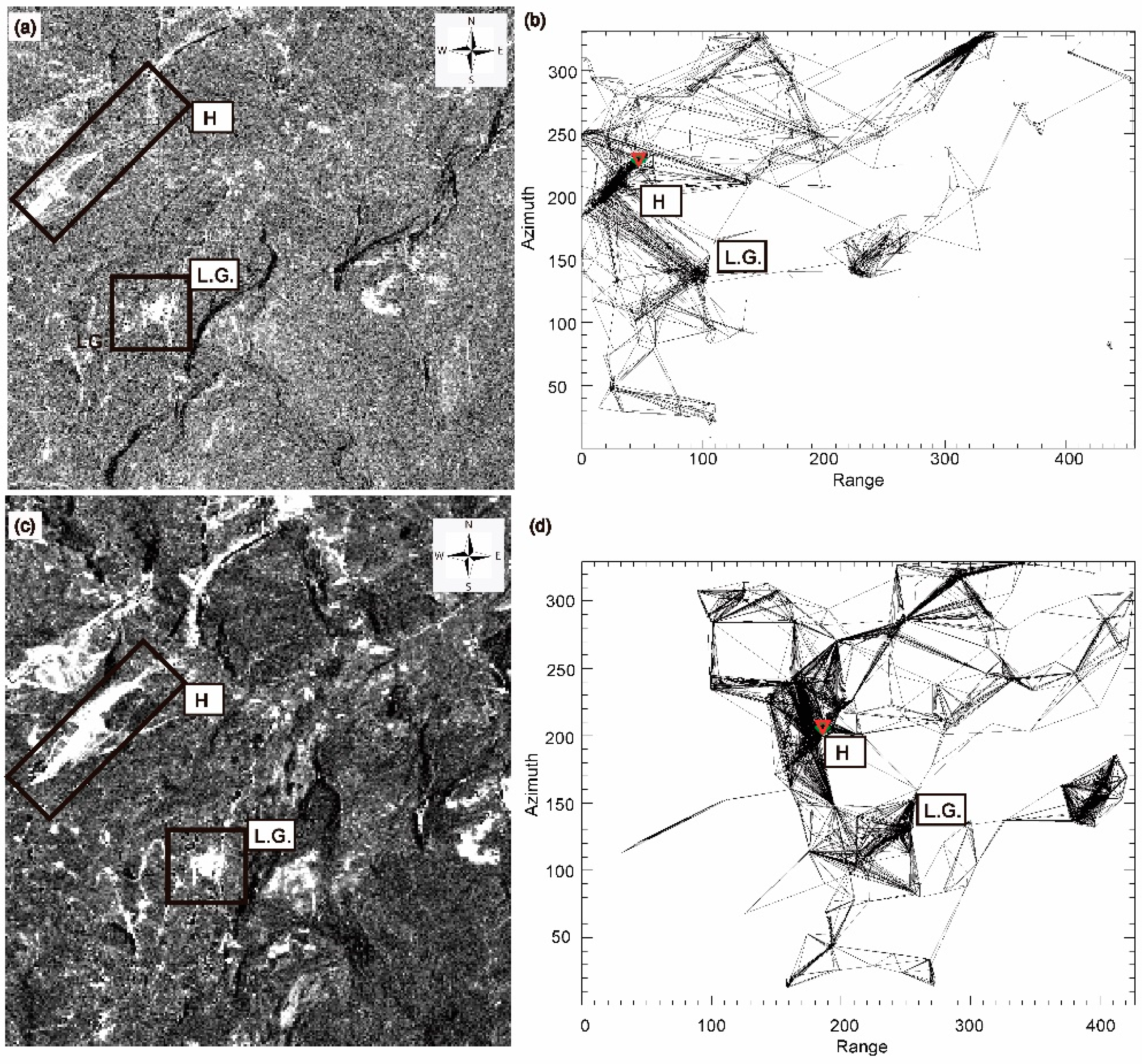
3.3. A-DInSAR Processing

A-DInSAR techniques use a stack of SAR images to extract the temporal evolution of the deformation. These techniques can be divided into two categories depending on how targets are selected in order to obtain the time series displacements: prevalent phase-coherent radar targets by amplitude stability or persistent scatter (PS) methods [47] and distributed targets by spatial coherence or small baseline subsets (SBAS) [48,49,50]. In general, the permanent scatters approach, which selects the PS candidates using the amplitude stability of pixels along time, is better suited for urban areas due to the high reflectivity and low decorrelation during man-made construction, but a minimum number of about 25 acquisitions is required [47]. The elevated cost of acquiring such a number of images from commercial X-band satellites, can be a limiting factor both for commercial and scientific uses. Spatial coherence techniques require a reduced set of images due to their capability to generate a larger number of interferograms. However, resolution is lowered due to the multilooking operation.

For Leintz Gatzaga landslide, we used the SUBSIDENCE-GUI processor which is based on the coherent pixels technique (CPT) developed at the remote sensing laboratory (RSLab) of the Universitat Politècnica de Catalunya (UPC) [51]. This approach has some similarities with the most-widely used Small Baselines Subset (SBAS), when we use multilooked images and the selection of pixels by coherence criteria (as in our case), but differs in the method used for velocity estimation. This method has provided good results in the past for similar test sites [14] and it was chosen because it has been proven to also work with a limited number of acquisitions, such as the set of TSX used here.

For areas with a high vegetation surface coverage, as the one presented in this paper, the user has to test different options to find the best compromise between pixels’ density and their quality. It is important to avoid, or at least reduce to the minimum, the number of pixels’ subsets (groups of pixels disconnected from the rest). Using multilook images and a coherence criteria to select those pixels with enough phase quality has a drawback: the chances of detecting isolated coherent scatters surrounded by low coherence areas is reduced. Achieving a good atmospheric phase filtering rely on having a well temporal distributed dataset and high pixel density (preferably with short spatial connections between pixels). For both SAR datasets, we used a coherence selection approach [50] with a 5 × 5 multi-look for the CSK and a 13 × 7 multi-look for the TSX, obtaining ground resolution pixels of approximately 10 × 10 m. For each dataset, we cropped the SAR images to an area of about 18 km² and co-registered to a common master geometry. We used a 5-m resolution DEM [46] to remove the topographic contribution. The mean coherences maps presented in Figure 10a,c show that coherence is very well preserved in the village, highway, and roads, while, as expected, vegetated areas are fully decorrelated. Overall, the density of coherent areas is large enough to obtain reliable deformation maps although long spatial connections between pixels had to be used (Figure 10b,d). The temporal filter is adjusted depending on the dataset characteristics, the image temporal sampling, to have at least enough temporal samples to average. The software used automatically expands the filter to include more images in case of temporal gaps in the data.

From the 43 CSK SAR images, we generated 90 interferograms, with a maximum temporal baseline of 250 days and spatial baselines below 500 m. From the 22 TSX SAR images, we generated 76 interferograms, with the same temporal and baselines restrictions. Connection diagrams of the interferograms of the CSK and TSX acquisitions is available in the Supplementary Material (Figure S1). We placed the reference point on the highway surface (red triangle in Figure 10b,d), where displacements are known to be inexistent. In order to select the CTs candidates, the model coherence threshold was set in 0.4 for the CSK dataset and 0.3 for the TSX. The next step of the CPT algorithm consists on carrying out a triangulation network in which nodes (CTs) are interconnected, with the objective of working with phase increments among CTs instead of absolute phases, which reduces unwrapping problems. In our test-site, some areas have low CTs density (less 1 × 10⁴ pixels/km²), so we employed redundant network strategies. CTs candidates were connected uniformly in all directions with arcs no longer than 800 m, forming a spider-web-like network [52], which added redundancy to the system and five additional links with respect to the Delaunay triangulation. A total subset of 1794 CTs for the CSK dataset and 1322 for the TSX passed the selection criteria.

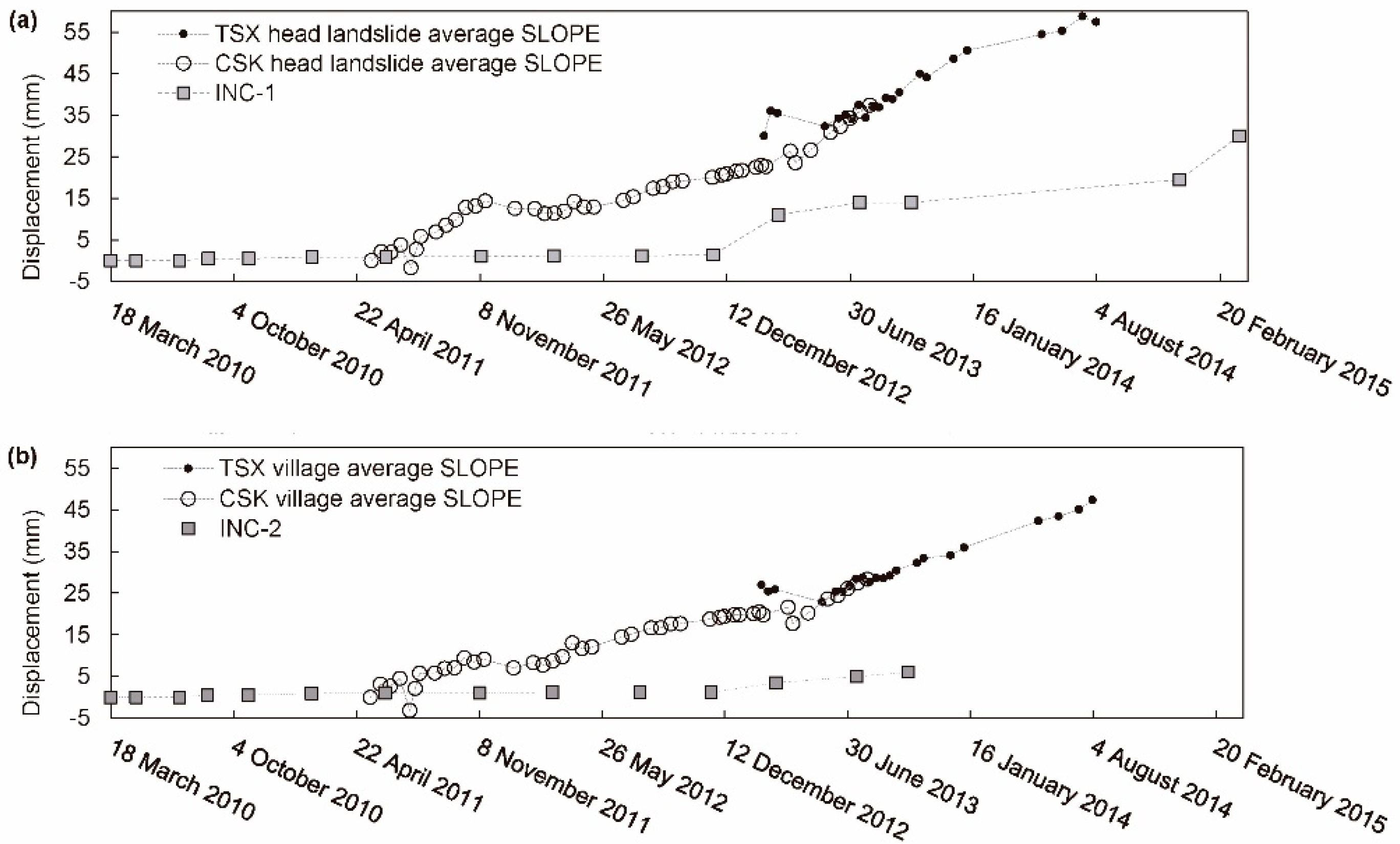
3.3.1. A-DInSAR Results

As expected from the pre-processing analysis, CTs of both datasets are restricted to urbanized areas and roads. Despite selecting just a few CTs that accomplished coherence criteria between the highway (were the reference point was placed) and the Leintz Gatzaga village, relatively dense connections were achieved (Figure 10b,d). However, other clusters of CTs within the cropped processed area have remained totally disconnected or with scarce connections, which compromise phase reliability and, hence, surface displacement rate estimations. Moreover, these clusters are located either out of the landslide area of interest, or over the confronting slope of the valley, so we have discarded them in the results and post processing analysis. From the total initial subsets of 1794 CTs of the CSK dataset and 1322 of the TSX, 926 and 658 CTs, respectively, remained after clipping the area of interest (Figure 11), which coincides with the extent of the clip used for the suitability analysis (2020 × 1440 m).

The standard deviation (s.d.) of mean LOS velocity values considering all coherent targets of the area of interest (2020 × 1440 m) is 5 mm/year for the CSK and 6 mm/year for the TSX datasets. The scene covers a wider area than the active landslide and includes stable zones. To the latter is added the fact that the landslide does not move homogeneously, which explains high s.d. values. We have assessed a stability threshold of 2 s.d. to establish active CT points. A point is considered active if |LOS velocity| > 2 s.d [53], where |LOS velocity| is the absolute LOS velocity value of each CT. Two standard deviation maps of the area of interest, one for each SAR dataset, are available in the Supplementary Material (Figure S2). We observe different active areas in the scene. The first one is Leintz Gatzaga landslide. It exhibits a mean LOS velocity of 6 mm/year for the extent of time monitored with the CSK dataset and 8 mm/year for the extent of time monitored with TSX. The s.d. of mean LOS velocity considering just the CT located within the landslide body, is 3 mm/year for CSK and 2 mm/year for TSX. Both monitoring periods overlap six months. The landslide does not move homogenously, but presents differential movements, also detected with other in situ monitoring techniques such as GNSS (Figure 5). These differences are highlighted in the standard deviation maps (Figure S2). Active zones concentrate in the head of the landslide and at the NE border of the village for both SAR datasets. The CSK dataset also presents active zones in the center of the village. The second active area is at the crown of a small secondary and individual landslide located to the South of Leintz Gatzaga village (labelled as S.L. in Figure 11). A small cluster of CT show mean LOS velocities up to 15 mm/year for the CSK dataset and up to 22.5 mm/year for the TSX dataset. We identified tension cracks at the crown of this secondary landslide in field work (Figures S2 and S3). To the east of the secondary landslide, CTs along the GI-3310 road also exhibit displacement, being more pronounced in the period monitored by the TSX. This area is covered by colluviums (Figure 1) where creeping and shallow movements are common. The third active area is Vitoria-Éibar highway. Even though is outside the area of influence of Leintz Gatzaga landslide, a brief analysis is unavoidable, as CPT processing has clearly detected movement at both soil cut slopes sides for the CSK dataset and to the east side for the TSX dataset. No measurements were taken with other monitoring techniques in this area, only in situ inspection was carried out. West side cut slope is composed by dark fine graded colluvium deposits and is currently reinforced with bolts. It is very scarcely vegetated and running water scars are present. Detected motion is extremely slow and it could be due to soil adjustment because the maximum load of the bolts was not reached during the SAR monitoring period or due other shallow process like surface washing. The east side cut slope exhibit a much greater rate of LOS movement that reaches up to 44 mm/year in the CSK dataset. Here a very small (50 × 100 m) local failure was identified; the main scarp can be clearly distinguished in the orthophoto. Surface movement detection at the cut slopes is a clear example on how remote sensing A-DInSAR techniques have the advantage of capturing unexpected or not previously registered with other techniques displacements. Other active zone was detected at the NW part of the scene, due to material for construction being quarried.

3.3.2. CT Detection Suitability Assessment

As described in the previous sub-section, we identified three main classes or categories of land cover (LC) according to the preservation of coherence along time and four classes of relief index (RI) according to geometrical distortions due to topography. To discern which was the best band combination to perform an automated land cover classification, we tested different options (Table 2) and computed the kappa coefficient for each of them. The higher value was obtained for image S2—20 August 2017, bands 2348, and 10 m resolution. Once both SAR datasets with the CPT software, were processed we overlapped the A-DInSAR results with the LC and RI maps in order to obtain the number of CTs that fail within each class. Results are shown in right columns of Table 2 (LC) and bottom rows of Table 3 (RI) in terms of percentage. Regarding the land cover, an average of 84% and 88.2% of the CT were detected in LC-1 class (urban), 13.3% and 9.3% in LC-2 (grasslands) and 2.7% and 2.5% in LC-3 (forest) for CSK and TXS datasets, respectively. This result is as expected; CTs will be detected at surfaces where coherence is preserved, as it the case of urban fabric. In general, the land cover maps with 20 m resolution cell detect more CTs at urban areas; the reason is because CTs have a resolution of 10 m after applying multilook so there are more chance that a CT fail within an area classified as urban. Note that georeferentation errors have not been taken into account. Regarding the RI, most of the CTs were detected in areas classified as RI-3, for both datasets.

Table 4. Average values of (from all the classifications) of the CTs distribution for each class with respect to the total amount of pixels of the studied scene.

Studied Scene Cell Resolution		CSK CT Distribution (%)				TSX CT Distribution (%)
		RI-1	RI-2	RI-3	RI-4	RI-1	RI-2	RI-3	RI-4
10 m	LC-1	0.0	2.8	21.1	16.0	0.0	1.6	17.2	11.5
	LC-2	0.0	0.3	1.4	1.7	0.0	0.1	0.5	0.8
	LC-3	0.0	0.0	0.2	0.2	0.0	0.0	0.3	0.4
		RI-1	RI-2	RI-3	RI-4	RI-1	RI-2	RI-3	RI-4
20 m	LC-1	0.0	6.6	77.7	57.3	0.0	3.2	60.3	44.1
	LC-2	0.0	0.0	5.6	4.4	0.0	0.0	1.6	3.2
	LC-3	0.0	0.1	0.7	1.0	0.0	0.0	0.4	0.5

shows the average proportion (from all the classifications) of the CTs detected in each class with respect to the total amount of pixels of the studied scene. Again, percentage values of 20m resolution cells are higher because the total amount of pixels of the studied scene are less (7373 pixels) than the finer resolution of 10 m (29,088 pixels). As for previous works [26], the influence of R index on CT density is strong for value under 0.3. We expected that the highest percentage was achieved by LC-1 and RI-4 combination. However, it was for RI-3. This might be due to two reasons: the presence of disconnected patches and loss of coherence of bare ground classified as LC-1.

From the information presented in Table 4, we have performed a qualitative classification of the X-band SAR visibility on the studied area taking into account LC and RI. We distinguish three classes, high visibility (HV), low visibility (LV), and no visibility (NV) as it is shown in

Table 5. Qualitative visibility classification. NV: no visible; LV: low visibility; HV: high visibility.

	RI-1	RI-2	RI-3	RI-4
LC-1	NV	LV	HV	HV
LC-2	NV	NV	LV	LV
LC-3	NV	NV	NV	NV

. Figure 12 shows a visibility classification map for both datasets using the LC classification obtained with the multiband image with better kappa coefficient (S2 image of 20 August 2017 with a resolution of 10 m and two-, three-, four-, and eight-band combination).

3.3.3. Post Processing Downslope Projection

A limitation of A-DInSAR is that movement is measured only in the LOS component. However, landslides typically address two movement components depending on the failure mechanism: the downslope direction in case of movements subparallel to the slope and the vertical direction in case of predominantly rotational movements [11]. In case of no availability of ascending and descending SAR images, which allow the separation of the displacement in the east–west horizontal and vertical components [8,9] we can apply the downslope projection method [11,36,54] provided that the movement is assumed to occur mainly towards the steepest slope. This procedure reduce geometrical distortions generated by the combination of the topography of mountainous environment and the satellite acquisition parameters [43]. Based on ground truth information and mechanical characterization of Leintz Gatzaga landslide, we assess that surface motion is mainly subparallel to the slope. Therefore, to fully exploit A-DInSAR displacement data, LOS velocity is projected along the steepest slope to obtain SLOPE velocity. We have applied this post-processing method only to the CTs located at the Leintz Gatzaga landslide and surroundings, discarding the highway area. We calculated the orientation (or aspect) and inclination of the slope needed to perform the downslope projection with a 5 m resolution DEM [46]. Figure 13 shows the SLOPE velocity maps of the two different time periods calculated with the geometrical parameters of each SAR dataset (Table 1). After performing the downslope projection, CT density has a reduction of about 35%, as we dismissed “uphill” direction values [36]. Average SLOPE velocity of the landslide calculated with the CSK dataset is 12 mm/year (6 mm/year of s.d.) and with the TSX dataset is 14 mm/year (5 mm/year of s.d.). Clearly, SLOPE velocity values are greater than their respective values in LOS. More importantly, differential movements are highlighted within the landslide. Maximum velocities are detected at the head of the landslide (close to INC-1), at the fronton court whose walls exhibit several cracks, and at the center and to the northwest of the village (Figure S3).

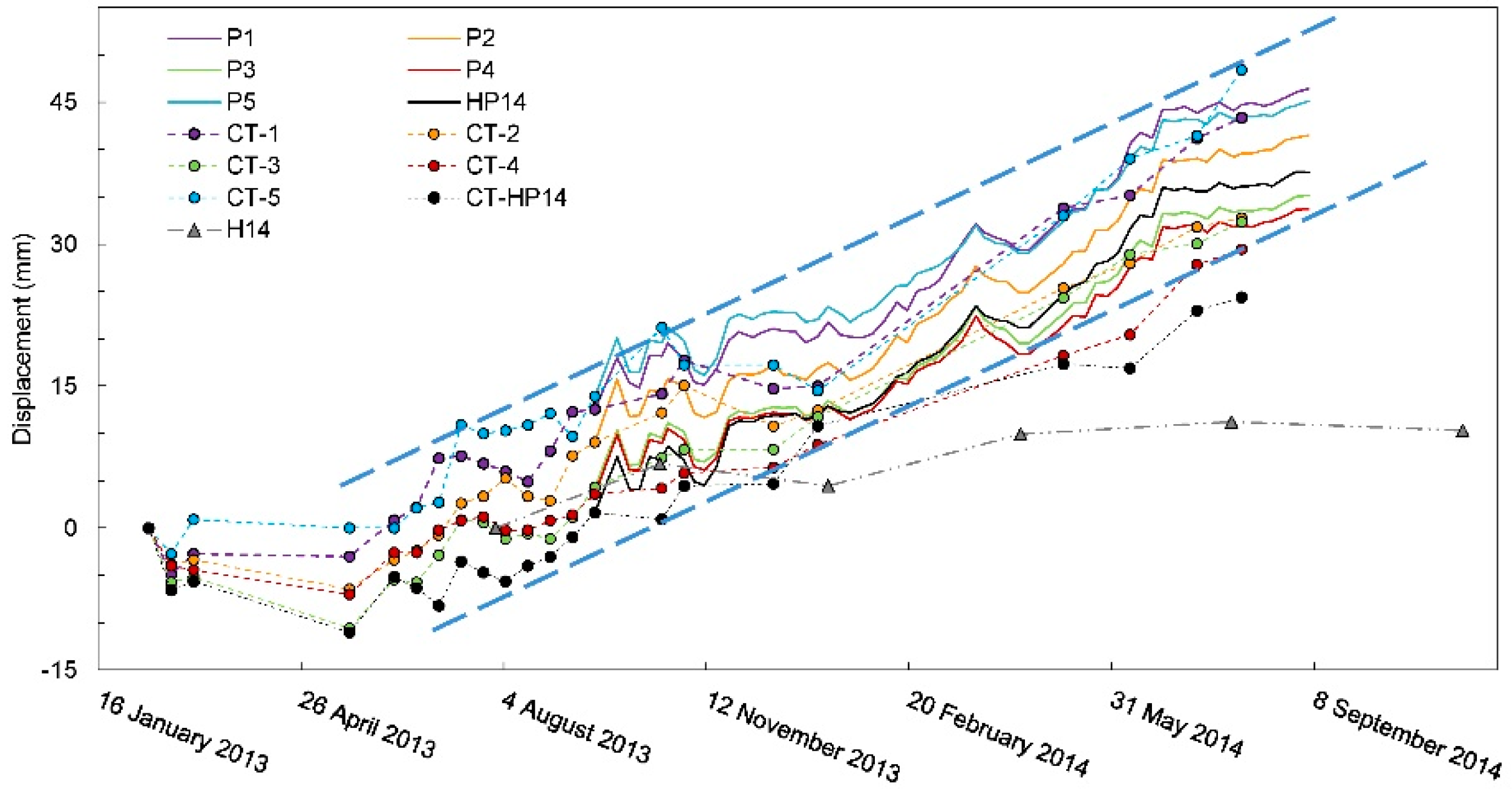
3.3.4. A-DInSAR Results Comparison to Ground Measurements

In this sub-section, we will compare overlapping satellite radar observations with ground truth data (Figure 3a) in terms of space distribution of movement and displacement time series. CSK dataset covers the time span 15 May 2011 to 1 August 2013 and TSX 10 February 2013 to 3 August 2014, overlapping almost six months. Both datasets present a similar space distribution of the landslide movement; higher rates are located at the head of the landslide, to the north of the village (fronton court and town hall), at the crown of a secondary slope failure (labelled S.L. in Figure 10 and Figure 12) and at the colluvium mass waste area around the GI-3310 road.

Inclinometers register the cumulated displacement along the line of maximum movement and they are referred to a stable surface under the sliding surface, while A-DinSAR represent the displacements measured at the surface in LOS direction with respect to a stable zone. This fact should be taken into account when comparing time series of both measurements. Inclinometric data overlaps both CSK and TSX datasets. Figure 14a show the average value of SLOPE time series displacements of the CTs located within a radius of 80 m to INC-1 at the head of the landslide. Figure 14b shows the average values of SLOPE displacement of all the CTs located within the village, where INC-2 is located. As discussed in the monitoring section, inclinometers do not register displacement until the rainy period of 20 November 2012–6 March 2013 (Figure 3b and Figure 13). However, surface displacements were measured with A-DInSAR since the first acquisition, being more pronounced at the head of the landslide than at the main body where the village settles, as it also happens in the inclinometers. The greater SLOPE displacement rates are registered between July 2011–November 2011 and since April 2013. Note that the stitching of CSK and TSX datasets time series of Figure 14 is based on the clear common trend between the end of May 2013 and beginning of August 2013. We have not applied any filter to the time series, so the first measures of TSX could be affected by noise, which might be the reason for differences in time series displacements during the time period from December 2012 to May 2013.

Ten crack gauges were installed on the facades of the line of buildings located to the north of the village. The maximum aperture was measured on one of the cracks of the fronton court, which is also the site were maximum displacements rates were measured by the CSK dataset in the village, up to 32.5–35 mm/year in downslope projection (Figure 13a). Regarding the TSX dataset, downslope velocities in the fronton court are between 17.5–12.5 mm/year, which are also higher than the average of the village, although the lower CTs density might mask higher rates of movement.

GNSS/HPL and EDM monitoring campaigns overlap with TSX dataset. Figure 15 shows the time series displacement of five prisms located to the north of the village (Figure 5) and the downslope projection of the CTs that are closer to each of them (Figure 13). Displacements measured by GNSS complemented with HPL at benchmark H14 (which houses prism HP14) are also shown. H14 and prisms displacements are expressed as the modulus of the three directions, which in all cases points downslope. Although time series are noisy (no filtering has been applied), the trend and amount of movement fits quite well between EDM and A-DInSAR measurements. GNSS/HPL measurement at H14 also captures the increment of movement from January 2014. However, the amount of displacement is less than the other techniques. In general, detected average velocity by GNSS/HPL is greater at the head and at the village, same as A-DInSAR. Maximum velocities were detected at benchmark H17 (Figure 5). A total displacement of 86 mm was measured for the period between 20 October 2013 and 11 January 2014. However CTs of the TSX dataset do not detect movement at that site probably due to aliasing [12], as there are four acquisitions in that period with a gap of 45 days between two of them. The measured values are included in a 15–20 mm wide strip, in agreement with the expected precision of DInSAR measurements [7].

4. Discussion

In this work, we propose a procedure that applies SAR data to obtain precise geotechnical monitoring results of site scale landslides affecting urban areas and/or civil infrastructures. The procedure is based on adequate SAR data selection, detailed site specification, high resolution visibility analysis, velocity projection along the steepest slope, and complemented with other monitoring data.

We determined that X-band SAR images were the best choice attending to the characteristics of the test landslide, the period wanted to be monitored and data availability. We acquired two datasets of CSK (Stripmap HIMAGE mode) and TSX (high resolution spotlight mode) images, covering the period from 15 May 2011 to 1 August 2013 and from 10 February 2013 to 3 August 2014, respectively. We carried out an advanced differential interferometric analysis to obtain velocities and displacement time series using the coherent pixel technique (CPT) and compare these results with data obtained from other monitoring instrumentation. We also applied the downslope projection method, as the data from other monitoring instrumentation indicates that the Leintz Gatzaga landslide moves towards the steepest slope. Both X-band datasets have shown capability to produce reliable mean LOS velocities and time series displacement maps for this area, thanks to its improved temporal and spatial resolution.

The dimension of cropped SAR image, broader than the landslide area, has allowed us to detect movements in unexpected zones, as is the case of the Vitoria–Eibar highway cut slopes. Average SLOPE velocity of the landslide calculated with the CSK dataset is 12 mm/year and with the TSX dataset is 14 mm/year, being both values greater than their respective in the LOS. Differential movements can be noticed within the landslide. Stable areas surrounding the landslide have also been detected. This information is very useful to geologist to make a more detailed landslide cartography. The most critical areas are the fronton court and the head of the secondary landslide. It can be noticed how movement increased along the GI-3310 road at the SW of the scene between CSK and TSK SLOPE results (Figure 12).

Comparison between A-DInSAR results and other instrumentation data in terms of space distribution of movement and displacement time series shows good agreement. Based on the results of this work, the main advantage of introducing A-DInSAR techniques in geotechnical monitoring campaigns is the dramatic enhancement of the density of surface measure points, allowing to identify differential movements of the instable zone and to detect previously unknown moving areas. The main disadvantages we found are the limitation of velocity measurability and the masked movements in the time series due to aliasing when there are long time gaps between SAR acquisitions. The enhancement of surface measuring point density is very useful to validate and adjust future stability analysis of the landslide [54].

Additionally to the proposed procedure, in this work we test new Sentinel-2 optical data to create high resolution land cover maps, which are useful for analyzing coherent targets’ detection of short wave length bands. The land coverage information, which is needed along with the topography for the visibility analysis, can be obtained from geographical databases at a low resolution, which is not useful to detailed site scale case studies. Therefore, we performed a supervised land use classification of 10 m and 20 m resolution S2 optical data, based upon three classes of coherence preservation. In order to assess which was the best choice of spectral band combination and epoch, we calculated the kappa coefficient to find the most accurate classification.

Our results (Table 2) show that the highest kappa coefficients are achieved with 10 m resolution and that the more the spectral bands used, kappa coefficients are higher. Regarding the two epochs tested, we obtained higher kappa coefficient with the optical S2 image acquired in 20 August 2017. We also analyzed what was the relative distribution of the CTs detected in each of the three land cover (LC) classes and the four relief index (RI) classes (Table 4). We observed that for values of RI that are less than 0.3, the topography is the main factor that rules CT detection, while for RI values higher than 0.3 is the type the land cover. This result is in concordance with previous works [26]. We created a qualitative visibility classification of the Leintz Gatzaga study area based upon our results (Table 5 and Figure 12) that can be used in other areas of the Deba Valley, where landslides of similar characteristics and occurring in similar scenarios (small urban patterns surrounded by vegetation), are common. However, there is an important point to take into account, which is CT connections. Even if an area has very good visibility, it can remain isolated if there are scarce connections between CTs, which can lead to detecting anomalous CTs due to unwrapping errors or not detecting them at all.

5. Conclusions

Slow moving landslides are a widespread geological hazard that can damage exposed urban elements. Engineering solutions are design either to reduce the vulnerability of those elements and/or to minimize the intensity of the hazard phenomena. For both cases, the mechanical behavior of the landslide must be understood and quantified in order to adopt the optimal solution. Surface and subsurface geotechnical monitoring of landslides can obtain valuable information of the spatial extension of the sliding body, the deepness of the sliding plane, the velocity, and the behavior in time. The surface extension of a landslide will help us to determine which urban elements are at risk and, in conjunction with the deepness of the sliding plane, the total volume of the displaced material. Both the volume of the mobilized material and the velocity will determine the intensity of the landslide phenomena and hence the potential severity of the damages to exposed vulnerable urban elements and/or civil infrastructures. Moreover, monitoring the movement allows us to analyze the landslide behavior in time and link velocity changes with physical processes, such as variation in water pore pressure due to rainfall or dynamic loads, softening of the soil, etc. This is fundamental to adjust physical-based models, be able to forecast the landslide behavior, and ultimately obtain future hazard scenarios and adopt appropriate solutions to reduce the risk.

The suitability of A-DInSAR for monitoring surface displacements of slow moving landslides at different scales is widely accepted, although its use has been restricted to academia, civil protection agencies, local authorities, and private companies are starting to include this tool of the operational monitoring of landslides. The scale at which we perform landslide assessments (regional or site scale) determines the minimum spatial resolution that is required to make a reliable analysis.

In this work, we present a practical guideline that applies A-DInSAR techniques to the operational geotechnical monitoring of site scale landslides affecting urban areas and/or civil infrastructures. We summarize this procedure as follows:

• A priori selection of the dataset according to the following aspects of the scenario:

  ○

  Type of land cover: will determine the radar sensor wavelength pulse selection.

  ○

  Spatial extent of the phenomena: will determine the minimum spatial resolution.

  ○

  Deformation dynamics: will determine the expected velocity and hence the wavelength pulse selection and minimum time between acquisitions.

  ○

  Geometry of the slope: will determine the acquisition mode of the SAR images.

  ○

  Period to be monitored: will determine if historical archives are needed (data availability) and to plan satellite data acquisition requests.

• Perform a qualitative visibility analysis of the selected SAR dataset with a GIS software, according to:

  ○

  Land cover: Use freely available S-2 optical image data to make supervised land cover classification. First identify the main classes of land cover according to the area of interest characteristics, the preservation of coherence among time or the amplitude reflectance (depending if SABS of PS approach are used) and the radar wavelength. We recommend using the higher resolution, closer to the ground resolution of the SAR data, and generating the multiband image (from which the supervised classification will be performed) with the maximum number of multispectral bands available.

  ○

  Relief geometrical distortion: Perform the relief index RI to detect geometrical distortions, using a DEM and the geometrical parameters of the SAR dataset

• Process the stack of SAR images with A-DInSAR: We have shown that performing a SBAS approach has the advantage of requiring less number of SAR images, which reduces the costs, although multilooking compromises the spatial resolution.
• Analyze the spatial distribution mean LOS velocity that will give information of the extension of the landslide, previously undetected unstable areas and differential movements.
• Perform the slope projection method if the movement occurs mainly along the steepest slope.
• When comparing and complementing A-DInSAR with other displacement monitoring data, take into account that A-DInSAR is measuring surface displacements; meanwhile other techniques, such as inclinometers, measure subsurface displacement at the rupture plane. If quantitative time series analysis is performed, all the data should be in the same projection. We must not forget that movements can be also masked by aliasing due to the sampling frequency.

In short, we have shown that A-DInSAR is a very powerful and versatile tool for geotechnical monitoring of landslides. However, we have to keep in mind that when detailed analysis is needed, a single monitoring technique is not enough. It has been demonstrate that high resolution LC classifications can be achieved with S-2 data. Future lines include the exploitation of current active C-band satellite Sentinel-1, of the European Space Agency (ESA), whose enhanced spatial resolution will allow to detect small coherent patches as the ones present in Leintz Gatzaga landslide. ESA products, such as Sentinel-1 and Sentinel-2 data, have the advantage of having an open access data policy.

References

1. Bryant, E.A. Natural Hazards, 1st ed.; N. Y. Cambridge University Press: New York, NY, USA, 1991; pp. 1–12. ISBN 0-521-37295-X. [Google Scholar]
2. UNEP/GRID-Geneva. Global Risk Data Platform. Available online: http://preview.grid.unep.ch (accessed on 18 February 2018).
3. Gili, J.A.; Corominas, J.; Rius, J. Using Global Positioning System techniques in landslide monitoring. Eng. Geol. 2000, 55, 167–192. [Google Scholar] [CrossRef]
4. Wieczorek, G.F.; Snyder, J.B. Monitoring slope movements. Geol. Monit. 2009, 245–271. [Google Scholar] [CrossRef]
5. Calò, F.; Ardizzone, F.; Castaldo, R.; Lollino, P.; Tizzani, P.; Guzzetti, F.; Lanari, R.; Angeli, M.-G.; Pontoni, F.; Manunta, M. Enhanced landslide investigations through advanced DInSAR techniques: The Ivancich case study, Assisi, Italy. Remote Sens. Environ. 2014, 142, 69–82. [Google Scholar] [CrossRef]
6. Hanssen, R.F. Radar Interferometry: Data Interpretation and Error Analysis; Springer Science & Business Media: Berlin, Germany, 2001; Volume 2. [Google Scholar]
7. Casu, F.; Manzo, M.; Lanari, R. A quantitative assessment of the SBAS algorithm performance for surface deformation retrieval from DInSAR data. Remote Sens. Environ. 2006, 102, 195–210. [Google Scholar] [CrossRef]
8. Lundgren, P.; Casu, F.; Manzo, M.; Pepe, A.; Berardino, P.; Sansosti, E.; Lanari, R. Gravity and magma induced spreading of Mount Etna volcano revealed by satellite radar interferometry. Geophys. Res. Lett. 2004, 31. [Google Scholar] [CrossRef] [Green Version]
9. Manzo, M.; Ricciardi, G.; Casu, F.; Ventura, G.; Zeni, G.; Borgström, S.; Berardino, P.; Del Gaudio, C.; Lanari, R. Surface deformation analysis in the Ischia Island (Italy) based on spaceborne radar interferometry. J. Volcanol. Geotherm. Res. 2006, 151, 399–416. [Google Scholar] [CrossRef]
10. Hilley, G.E.; Bürgmann, R.; Ferretti, A.; Novali, F.; Rocca, F. Dynamics of slow-moving landslides from permanent scatterer analysis. Science 2004, 304, 1952–1955. [Google Scholar] [CrossRef] [PubMed]
11. Colesanti, C.; Wasowski, J. Investigating landslides with space-borne Synthetic Aperture Radar (SAR) interferometry. Eng. Geol. 2006, 88, 173–199. [Google Scholar] [CrossRef]
12. Wasowski, J.; Bovenga, F. Investigating landslides and unstable slopes with satellite Multi Temporal Interferometry: Current issues and future perspectives. Eng. Geol. 2014, 174, 103–138. [Google Scholar] [CrossRef]
13. Cascini, L.; Fornaro, G.; Peduto, D. Analysis at medium scale of low-resolution DInSAR data in slow-moving landslide-affected areas. ISPRS J. Photogramm. Remote Sens. 2009, 64, 598–611. [Google Scholar] [CrossRef]
14. Iglesias, R.; Monells, D.; Centolanza, G.; Mallorquí, J.J.; Fabregas, X.; Aguasca, A. Landslide monitoring with spotlight TerraSAR-X DATA. In Proceedings of the 2012 IEEE International Geoscience and Remote Sensing Symposium (IGARSS), Munich, Germany, 22–27 July 2012; pp. 1298–1301. [Google Scholar]
15. Iglesias, R.; Monells, D.; Centolanza, G.; Mallorqui, J.; Fabregas, X.; Aguasca, A. Down-slope combination of orbital and ground-based DInSAR for the efficient monitoring of slow-moving landslides. In Proceedings of the 10th European Conference on Synthetic Aperture Radar (EUSAR 2014), Berlin, Germany, 3–5 June 2014; pp. 1–4. [Google Scholar]
16. Remondo, J.; González, A.; De Terán, J.R.D.; Cendrero, A.; Fabbri, A.; Chung, C.-J.F. Validation of landslide susceptibility maps; examples and applications from a case study in Northern Spain. Nat. Hazards 2003, 30, 437–449. [Google Scholar] [CrossRef]
17. Ábalos, B.; Alkorta, A.; Iríbar, V. Geological and isotopic constraints on the structure of the Bilbao anticlinorium (Basque–Cantabrian basin, North Spain). J. Struct. Geol. 2008, 30, 1354–1367. [Google Scholar] [CrossRef]
18. Euroestudios. Informe Geotécnico para Control del Deslizamiento Existente entre los PPKK 4,550-5,630 de la GI-3310 y Tramo Inicial de la GI-3681 en Leintz Gatzaga (Gipuzkoa); Euroestudios: Madrid, Spain, 2011; p. 119. [Google Scholar]
19. Bru, G.; Gascón, B.; Camacho, A.; Prieto, J.F.; Mallorqui, J.; Morales, A.; Fernández, J. Deslizamiento de Leintz Gatzaga: Instrumentación geotécnica y monitorización del movimiento con técnicas terrestres y espaciales. Proyecto EOSLIDE. Ing. Civ. 2015, 180, 55–75. [Google Scholar]
20. Euroestudios. Recopilacion de Informacion Geotécnica y Propuestas de Control Carretera GI-3681 en Leintz Gatzaga (Gipuzkoa); Euroestudios: Madrid, Spain, 2009; p. 196. [Google Scholar]
21. Cruden, D.M.; Varnes, D.J. Landslides: Investigation and mitigation. Chapter 3: Landslide types and processes. Transportation Research Board Special Report, 15 July 1996. [Google Scholar]
22. Fell, R. Landslide risk assessment and acceptable risk. Can. Geotech. J. 1994, 31, 261–272. [Google Scholar] [CrossRef]
23. Osmanoğlu, B.; Sunar, F.; Wdowinski, S.; Cabral-Cano, E. Time series analysis of InSAR data: Methods and trends. ISPRS J. Photogramm. Remote Sens. 2016, 115, 90–102. [Google Scholar] [CrossRef]
24. Farina, P.; Colombo, D.; Fumagalli, A.; Marks, F.; Moretti, S. Permanent Scatterers for landslide investigations: Outcomes from the ESA-SLAM project. Eng. Geol. 2006, 88, 200–217. [Google Scholar] [CrossRef]
25. Colombo, A.; Mallen, L.; Pispico, R.; Giannico, C.; Bianchi, M.; Savio, G. Mappatura regionale delle aree monitorabili mediante l’uso della tecnica PS. In Proceedings of the 10 National Conference ASITA, Bolzano, Italy, 14–17 November 2006. ISBN/ISSN:88-900943-0-3-2006. [Google Scholar]
26. Notti, D.; Meisina, C.; Zucca, F.; Colombo, A. Models to predict Persistent Scatterers data distribution and their capacity to register movement along the slope. In Proceedings of the Fringe 2011 Workshop, ESRIN SP-697, Frascati, Italy, 19–23 September 2011; pp. 17–23. [Google Scholar]
27. Plank, S.; Singer, J.; Minet, C.; Thuro, K. Pre-survey suitability evaluation of the differential synthetic aperture radar interferometry method for landslide monitoring. Int. J. Remote Sens. 2012, 33, 6623–6637. [Google Scholar] [CrossRef]
28. Plank, S.; Singer, J.; Thuro, K. Assessment of number and distribution of persistent scatterers prior to radar acquisition using open access land cover and topographical data. ISPRS J. Photogramm. Remote Sens. 2013, 85, 132–147. [Google Scholar] [CrossRef]
29. Strozzi, T.; Farina, P.; Corsini, A.; Ambrosi, C.; Thüring, M.; Zilger, J.; Wiesmann, A.; Wegmüller, U.; Werner, C. Survey and monitoring of landslide displacements by means of L-band satellite SAR interferometry. Landslides 2005, 2, 193–201. [Google Scholar] [CrossRef]
30. IGN. Ortophoto PNOA, Sheet No. 0112, 2017. Available online: http://ign.es (accessed on 25 October 2017).
31. Diputación Foral de Gipuzkoa. Cadastre. Available online: http://www4.gipuzkoa.net/ogasuna/catastro/presenta.asp (accessed on 10 September 2017).
32. Sansosti, E.; Berardino, P.; Bonano, M.; Calò, F.; Castaldo, R.; Casu, F.; Manunta, M.; Manzo, M.; Pepe, A.; Pepe, S. How second generation SAR systems are impacting the analysis of ground deformation. Int. J. Appl. Earth Obs. Geoinf. 2014, 28, 1–11. [Google Scholar] [CrossRef]
33. Cascini, L.; Fornaro, G.; Peduto, D.; Ferlisi, S.; Di Nocera, S. A new approach to the use of DinSAR data to study slow-moving landslides over large areas. In Proceedings of the Fringe 2009 Workshop, Frascati, Italy, 30 November–4 December 2010. [Google Scholar]
34. Ferretti, A.; Fumagalli, A.; Novali, F.; Prati, C.; Rocca, F.; Rucci, A. A new algorithm for processing interferometric data-stacks: SqueeSAR. IEEE Trans. Geosci. Remote Sens. 2011, 49, 3460–3470. [Google Scholar] [CrossRef]
35. García-Davalillo, J.C.; Herrera, G.; Notti, D.; Strozzi, T.; Álvarez-Fernández, I. DInSAR analysis of ALOS PALSAR images for the assessment of very slow landslides: The Tena Valley case study. Landslides 2014, 11, 225–246. [Google Scholar] [CrossRef]
36. Herrera, G.; Gutiérrez, F.; García-Davalillo, J.; Guerrero, J.; Notti, D.; Galve, J.; Fernández-Merodo, J.; Cooksley, G. Multi-sensor advanced DInSAR monitoring of very slow landslides: The Tena Valley case study (Central Spanish Pyrenees). Remote Sens. Environ. 2013, 128, 31–43. [Google Scholar] [CrossRef]
37. Borràs, J.; Delegido, J.; Pezzola, A.; Pereira, M.; Morassi, G.; Camps-Valls, G. Clasificación de usos del suelo a partir de imágenes Sentinel-2. In Revista de Teledetección; Universitat Politècnica de València: València, Spain, 2017; pp. 55–66. [Google Scholar]
38. Mather, P.M.; Koch, M. Computer Processing of Remotely-Sensed Images: An Introduction; John Wiley & Sons: Hoboken, NJ, USA, 2011. [Google Scholar]
39. Cohen, J. A coefficient of agreement for nominal scales. Educ. Psychol. Meas. 1960, 20, 37–46. [Google Scholar] [CrossRef]
40. Foody, G.M. Thematic map comparison. Photogramm. Eng. Remote Sens. 2004, 70, 627–633. [Google Scholar] [CrossRef]
41. Sansosti, E. A simple and exact solution for the interferometric and stereo SAR geolocation problem. IEEE Trans. Geosci. Remote Sens. 2004, 42, 1625–1634. [Google Scholar] [CrossRef]
42. Ferretti, A.; Monti-Guarnieri, A.; Prati, C.; Rocca, F.; Massonet, D. InSAR Principles—Guidelines for SAR Interferometry Processing and Interpretation; European Space Reseach and Technology Centre (ESTEC): Noordwijk, The Netherlands, 2007; Volume 19. [Google Scholar]
43. Notti, D.; Davalillo, J.; Herrera, G.; Mora, O. Assessment of the performance of X-band satellite radar data for landslide mapping and monitoring: Upper Tena Valley case study. Nat. Hazards Earth Syst. Sci. 2010, 10, 1865–1875. [Google Scholar] [CrossRef] [Green Version]
44. Cigna, F.; Bateson, L.B.; Jordan, C.J.; Dashwood, C. Simulating SAR geometric distortions and predicting Persistent Scatterer densities for ERS-1/2 and ENVISAT C-band SAR and InSAR applications: Nationwide feasibility assessment to monitor the landmass of Great Britain with SAR imagery. Remote Sens. Environ. 2014, 152, 441–466. [Google Scholar] [CrossRef]
45. Bianchini, S.; Herrera, G.; Mateos, R.M.; Notti, D.; Garcia, I.; Mora, O.; Moretti, S. Landslide activity maps generation by means of Persistent Scatterer Interferometry. Remote Sens. 2013, 5, 6198–6222. [Google Scholar] [CrossRef]
46. IGN. Digital Elevation Model, LIDAR 5m, Sheet No. 0112. Available online: http://ign.es (accessed on 5 May 2017).
47. Ferretti, A.; Prati, C.; Rocca, F. Permanent scatterers in SAR interferometry. IEEE Trans. Geosci. Remote Sens. 2001, 39, 8–20. [Google Scholar] [CrossRef] [Green Version]
48. Berardino, P.; Fornaro, G.; Lanari, R.; Sansosti, E. A new algorithm for surface deformation monitoring based on small baseline differential SAR interferograms. IEEE Trans. Geosci. Remote Sens. 2002, 40, 2375–2383. [Google Scholar] [CrossRef]
49. Mora, O.; Mallorqui, J.J.; Broquetas, A. Linear and non-linear terrain deformation maps from a reduced set of interferometric SAR images. IEEE Trans. Geosci. Remote Sens. 2003, 41, 2243–2253. [Google Scholar] [CrossRef]
50. Lanari, R.; Mora, O.; Manunta, M.; Mallorqui, J.J.; Berardino, P.; Sansosti, E. A small baseline DInSAR approach for investigating deformations on full resolution SAR interferograms. IEEE Trans. Geosci. Remote Sens. 2004, 42, 1377–1386. [Google Scholar] [CrossRef]
51. Blanco, P.; Mallorqui, J.J.; Duque, S.; Monells, D. The Coherent Pixels Technique (CPT): An advanced DInSAR technique for nonlinear deformation monitoring. Pure Appl. Geophys. 2008, 165, 1167–1193. [Google Scholar] [CrossRef]
52. Iglesias, R.; Aguasca, A.; Fabregas, X.; Mallorqui, J.J.; Monells, D.; López-Martínez, C.; Pipia, L. Ground-Based Polarimetric SAR Interferometry for the Monitoring of Terrain Displacement Phenomena–Part I: Theoretical Description. IEEE J. Sel. Top. Appl. Earth Obs. Remote Sens. 2015, 8, 980–993. [Google Scholar] [CrossRef]
53. Barra, A.; Solari, L.; Béjar-Pizarro, M.; Monserrat, O.; Bianchini, S.; Herrera, G.; Crosetto, M.; Sarro, R.; González-Alonso, E.; Mateos, R.M. A Methodology to Detect and Update Active Deformation Areas Based on Sentinel-1 SAR Images. Remote Sens. 2017, 9, 1002. [Google Scholar] [CrossRef]
54. Cascini, L.; Fornaro, G.; Peduto, D. Advanced low-and full-resolution DInSAR map generation for slow-moving landslide analysis at different scales. Eng. Geol. 2010, 112, 29–42. [Google Scholar] [CrossRef]
Figure 1. Geomorphological and geological sketch map of Leintz Gatzaga landslide area with location of geotechnical instrumentation (inclinometers, piezometers, and compiled boreholes from previous works). Blue arrows indicate direction of movement. Cross section marked in purple is shown below (modified from [18]).
Remotesensing 10 00936 g001
Figure 2. Paleo-landslide evolution scheme. (a) Original slope profile; (b) Current slope profile [10].
Remotesensing 10 00936 g002
Figure 3. (a) Measuring dates of the landslide cinematic monitoring campaigns performed with: in situ (EDM, GNSS/HPL, crack gauges, inclinometers) and remote sensing (A-DinSAR) techniques. The temporal coverage of the A-DinSAR techniques is 15 May 2011–1 August 2013 for the COSMO-SkyMed dataset and 10 February 2013–3 August 2014 for the TerraSAR-X dataset; (b) Time periods of maximum velocities registered by in-situ monitoring campaigns. Accumulate precipitation data (pp) in 3 days and 30 days is also displayed, in order to compare pp peaks with maximum velocities.
Remotesensing 10 00936 g003
Figure 4. Displacement graph for inclinometer INC-3, located at the head of the landslide, with correspondent core sample lithostratigraphic column. The dotted rectangle represents the depth and thickness of the shear band.
Remotesensing 10 00936 g004
Figure 5. Location of GNSS and prism reflector control points. E1 refers to electronic distance measurement (EDM) robotic station. Arrows indicate the direction of the movement detected by GNSS on the horizontal plane and are scaled with respect to the total accumulated displacement of the sixth campaign, 20 November 2014. Inset graph shows the arithmetic mean of the horizontal displacements measured in benchmarks H17, H18, and H19.
Remotesensing 10 00936 g005
Figure 6. Flow chart of the proposed procedure. * A detailed description of the different algorithms categories of A-DInSAR processing can be found in [23]. ** To apply if the movement occurs mainly along the steepest slope.
Remotesensing 10 00936 g006
Figure 7. (a) Orthophoto of Leintz Gatzaga landslide area. Dark green zones correspond to forest (F) and light green yellowish to grasslands (G). Roads are delineated in black and landslide lobes in light blue. Urban fabric is depicted in pink. (b) Multiband image obtained by the combination of bands 2, 3, 4, and 8 of a S2 optical image acquired in 20 August 2017 (10 m pixel size). (c) Land cover classes obtained by supervised classification from multiband S2 image shown in panel 6b: pink for urban or bare ground (coherence is expected to be very well preserved), light green for grass (coherence is expected to be bad preserved), dark green for forest (coherence is expected to be completely loss).
Remotesensing 10 00936 g007
Figure 8. RI maps or geometrical visibility maps for (a) CSK and (b) TSX ascending datasets (resolution 10 m). Black arrows indicate right side-looking antenna of the ascending satellite orbits.
Remotesensing 10 00936 g008
Figure 9. Relative distribution in the studied scene of land cover (from classification obtained from S2-20 August 2017, bands 2348 and 10 m resolution that has the better kappa coefficient) and RI (10 m resolution) classes of (a) CSK dataset geometric parameters and (b) TSX dataset geometric parameters. Pixel density of each class with respect to the total amount of 29,088 pixels of the studied scene are labelled in terms of percentage.
Remotesensing 10 00936 g009
Figure 10. (a) Coherence map of CSK data. Black color indicates 0 value, white color 1. (b) CT connection graph obtained with spider web-like triangulation of CSK data. (c) Coherence map of TSX data. (d) CT connection graph obtained with spider web-like triangulation of TSX. Leintz Gatzaga village (L.G.) and Vitoria-Éibar highway (H) are located in all figures. The reference point is depicted in red.
Remotesensing 10 00936 g010
Figure 11. LOS velocity maps of the area of interest of (a) CSK and (b) TSX datasets. Positive values indicate movement going away from satellite. A secondary landslide located to the South of Leintz Gatzaga village is labelled as S.L. Black arrows indicate right side-looking antenna of the ascending satellite orbits.
Remotesensing 10 00936 g011
Figure 12. Visibility classification map for (a) CSK and (b) TSX datasets.
Remotesensing 10 00936 g012
Figure 13. SLOPE velocity maps. (a) Obtained with CSK dataset: general view of the landslide (left) and zoom of the village (right). (b) Obtained with TSX dataset: general view of the landslide (left) and zoom of the village with prisms reflectors locations (right).
Remotesensing 10 00936 g013
Figure 14. (a) Average SLOPE displacements of the CSK and TSX CTs that are closer to INC-1 within a radius of 80 m. (b) Average SLOPE displacements of the CSK and TSX CTs within the village where INC-2 is located.
Remotesensing 10 00936 g014
Figure 15. Displacements time series of: prisms (P1, P2, P3, P4, P5, HP14) measured by EDM, downslope projection of the CTs that are closer to each prism obtained by DInSAR processing of the TSX dataset and benchmark H14 (that houses prism HP14) measured by GNSS complemented with HPL. See points location in Figure 13b. Note the first measures of the prisms have been set at the value of displacement of the correspondent CT.
Remotesensing 10 00936 g015