1. Introduction
Nowadays, many practical applications, such as optical remote sensing application [
1], weather prediction [
2], precipitation estimation [
3] and deep space climate observatory mission [
4], require accurate cloud observation techniques. However, cloud observation is currently performed by professional observers, which is traditionally labor-intensive and prone to producing observation errors. Hence, many efforts have been made for automatic cloud observation [
5,
6,
7,
8,
9]. As a key issue of cloud observation, the automatic cloud type classification is a very challenging task due to extremely variant cloud appearances under different atmospheric conditions and therefore it is still under development.
Different measuring instruments have been employed by numerous researchers to obtain the necessary data for cloud classification. The measuring instruments consist of ground-based and satellite-based equipment [
10]. The satellite-based equipment has a wide view field and provides large-scale cloud information over continents, while the ground-based equipment has a limited view field and is usually fixed at a specific location for cloud observation. It therefore appears reasonable to consider ground-based instruments for continuous local cloud observation. The existing ground-based sky imaging devices include whole-sky imager (WSI) [
11], total-sky imager (TSI) [
12], infrared cloud imager (ICI) [
13], all-sky imager (ASI) [
14], whole-sky infrared cloud-measuring system (WSIRCMS) [
15], etc. They could produce the most available amount of cloud data and, consequently, offer researchers an opportunity to understand the cloud conditions better.
Benefiting from these cloud data, the ground-based cloud classification methods have emerged in large numbers. Buch et al. [
16] treated texture measures, position information and pixel brightness as features, and employed binary decision trees to classify cloud types. Heinle et al. [
17] selected seven color features, four textural features and cloud cover ratio, resulting in twelve features, to distinguish the cloud into seven classes. Liu et al. [
18] extracted several structural features from the segment images and edge images, such as cloud gray mean value, cloud fraction, edge sharpness, and cloud mass and gap distribution parameters. Singh and Glennen [
19] evaluated five different feature extraction methods for cloud classification, namely autocorrelation, co-occurrence matrices, edge frequency, Law’s features and primitive length. Liu et al. [
20,
21,
22,
23] presented several approaches to learn discriminative texture features, such as an ensemble approach of multiple random projections, the salient local binary pattern, the soft-signed sparse coding and the mutual information learning features. Zhuo and Cao [
24] proposed a three-step algorithm, including applying the preprocessing color census transform, capturing global rough structure information and obtaining the cloud type. Xiao et al. [
25] proposed to extract the texture, structure, and color visual descriptors for cloud representation in a joint manner. Specifically, these features contain scale invariant feature transform (SIFT) [
26], the census transform histogram and some statistical color features.
Recently, the deep convolutional neural networks (CNNs) have shown promising capabilities in many research tasks [
27,
28,
29,
30,
31,
32]. The most competitive advantage of deep CNNs is that they are capable of learning high-level features adaptively from the raw input data through multiple nonlinear transformations. Thus, they are automatically able to capture the representative features to a great extent. Inspired by this property, several researchers resort to the deep CNNs to extract visual features for ground-based cloud classification, and promising results have been achieved. For example, Ye et al. [
33] first extracted the deep visual features from convolutional layers and then adopted a series of methods, i.e., fisher vector encoding and cloud pattern mining and selection, to improve the differentiation of different cloud types. Shi et al. [
34] employed the max or average pooling scheme on the feature maps to extract deep convolutional activations-based features. It should be noted that these features are not only from the shallow convolutional layers but also from the deep convolutional layers of the CNN. The classification performance of a fully connected (FC) layer for ground-based cloud is evaluated as well.
However, most existing methods only employ visual features to distinguish the ground-based cloud, which is not robust to environmental factors. For example,
Figure 1 shows two cloud images with the same type (cumuls), yet they appear different in shapes, illuminations, and occlusions.
Figure 1c shows their corresponding multimodal information, where we can see that the multimodal information is rather stable and less affected by environmental factors. Moreover, the cloud type is influenced by these multimodal information, i.e., temperature, humidity, pressure and wind speed. Specifically, air is made up of molecules of elements in gaseous state and minute dust particles. The rays of the sun heat the earth surface, which in turn heats the air. The more heat, the faster the molecules move, causing different in temperature and air pressure. The unequal heating of the atmosphere results in air masses with different densities of thicknesses. Humidity is the measure of water vapor in the atmosphere. When air rises and cools, clouds form and humidity increases. Wind is moving air caused by differences in air pressure, which moves from an area of higher pressure to an area of lower pressure. The greater the differences in air pressure, the greater the wind speed. Winds bring in different air masses and therefore form different cloud patterns. Hence, the multimodal information could describe the cloud completely and fusing the visual features with the multimodal information could further improve the classification performance.
Information fusion has shown promising performances in different research fields [
35,
36,
37,
38,
39]. The existing approaches usually fuse information at three levels, i.e., the feature level, matching-score level and decision level. For the score-level and decision level, some information may be lost in the fusion process as the multi-dimensional features are simply compressed into one match score or a final decision. For the feature level fusion, the resulting feature set is with richer information of the input data, and therefore fusion at such level is most likely to provide the desired classification performances. In general, the existing feature level fusion techniques can be classified into two subsidiary sets, i.e., feature extraction-based and feature selection-based methods [
40]. For the feature extraction-based method, several feature sets are grouped into one union-vector. For the feature selection-based method, all features are primarily aggregated together and then an appropriate method is adopted to select features. CNNs are treated as a kind of feature selection-based methods because CNNs could learn the complementary representations from intermediate layers. However, few works have been done for multimodal ground-based cloud classification. The major challenges in fusing the cloud visual features and the multimodal information can be contributed to two aspects. On the one hand, the nature of the cloud image and the multimodal information is radically different. Concretely, the mathematical expression of cloud image is a matrix, while the multimodal information is a vector. On the other hand, they contain different semantic information. Hence, CNNs cannot be directly applied to cloud classification with multimodal information.
In this paper, a novel deep model named joint fusion convolutional neural network (JFCNN) is proposed for multimodal ground-based cloud classification. The proposed JFCNN mainly consists of two subnetworks (vision subnetwork and multimodal subnetwork) and one joint fusion layer. The vision subnetwork utilizes the CNN model for learning visual features, which could process the matrix data. Meanwhile, the multimodal subnetwork employs multilayer perceptron to learn the multimodal information, which is designed for the vector data input. For the subsequent fusion, the outputs of two subnetworks possess the same dimension. To combine the strengths of the two subnetworks and leverage their complementary properties, we propose a novel layer named joint fusion layer, which has the ability to fuse the heterogeneous features. We only utilize one loss function to optimize the proposed JFCNN, which could jointly learn the discriminative features for cloud images and multimodal data under one framework. The experimental results indicate the effectiveness of the proposed method for the multimodal ground-based cloud classification.
The rest of the paper is arranged as follows. In
Section 2, we describe the proposed JFCNN architecture and provide the implementation details.
Section 3 presents a brief introduction about the dataset and baselines followed by the analyses of experimental results. Finally, we conclude this paper in
Section 4.
2. Methods
In this section, we first describe the overall framework of the proposed JFCNN. Then, we introduce the feature fusion strategy for ground-based cloud data. Finally, the implementation details are presented.
2.1. Overall Architecture
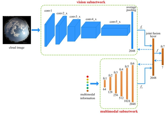
The overall architecture of the proposed JFCNN is shown in
Figure 2. It mainly consists of five parts, i.e., two subnetworks, one joint fusion layer, one FC layer and the loss function. The vision subnetwork is used for learning cloud visual features, which is based on the widely-used ResNet-50 [
41]. The architecture of ResNet-50 is summarized in
Table 1. The building block shown in the brace of the third column includes three convolutional layers. For example,
conv3_
x has four building blocks. For each building block in
conv3_
x, 1 × 1, 3 × 3 and 1 × 1 indicate the size of filters, respectively, and 128, 128 and 256 represent the number of filter banks, respectively. In addition, the max pooling layer and the average pooling layer are connected to the outputs of the first and last convolutional layers, respectively. More information about the ResNet-50 can be referred to [
41]. Note that, in the vision subnetwork, the final FC layer is removed, and the output of the average pooling layer is treated as the input of the joint fusion layer, which is a 2048-dimensional vector.
The multimodal subnetwork is designed for learning multimodal information of ground-based cloud and it contains six FC layers. The number of neurons in fc1 is 64 and increases by a factor of 2 up to 2048 in fc6. The FC layer could be considered as a special case of convolutional layer with the kernel size of 1 × 1. The output of fc6 is fed into the joint fusion layer, which is a 2048-dimensional vector as well.
After learning the visual features and the multimodal features, the join fusion layer is proposed to integrate them. The joint fusion layer is formulated as
where
and
are the outputs of the vision subnetwork and the multimodal subnetwork, respectively, and
is used to balance the significance of multimodal feature
. Note that the dimensions of
f,
and
are all 2048. We add an FC layer (
) after the joint fusion layer and the neuron number of
is consistent with the number of cloud classes.
For the classification task of multimodal ground-based cloud, we apply the softmax operator on the output of
to generate a probability distribution with values between 0 and 1 over
K cloud classes. The softmax operator is formulated as
where
K is the number of cloud classes,
is the output value of the
k-th neuron in
, and
is the predicted probability value of the
k-th class.
We employ the cross-entropy loss to measure the performance of the proposed JFCNN, and it is formulated as
where
is the ground-truth probability.
= 0 for all
k except
= 1 when
j is the ground-truth label. The cross-entropy loss will give a high penalty when the predicted probability diverges from the ground-truth label. Thereby, minimizing Equation (
3) is equivalent to maximizing the expected log-likelihood of a label, where the label is selected according to the maximum distribution value
.
2.2. Feature Fusion
After training the proposed JFCNN, we extract
as the visual features, and
as the multimodal features. Both features contain some complementary information and describe different characteristics of the ground-based cloud. Hence, combining them could further improve the discriminative ability of features. The integration features, which are used as the final cloud features, can be formulated as
where
is the fusion function. For simplicity and efficiency,
is formulated as
where
indicates the operation of concatenating two vectors, and
is the coefficient to adjust the significance of the multimodal features.
In other words, the proposed JFCNN has two great properties. Firstly, the two subnetworks could learn the discriminative features for heterogeneous features. Concretely, the input cloud image is a matrix, while the input multimodal information is a vector. The two kinds of features contain different semantic information. Thus, cloud images and multimodal information are heterogeneous features. The two subnetworks could learn them at the same time, and obtain the discriminative features. Secondly, the joint fusion layer could make it possible to fuse the heterogeneous information in the framework of CNN.
2.3. Implementation Details
For the ground-based cloud visual information, we first resize all the training ground-based images to 256 × 256 with the preserved aspect ratio. Then, all the images are subtracted from the mean values computed on the images in the training set in RGB channels. Finally, each training image is randomly cropped into 224 × 224. The multimodal information includes six aspects, i.e., temperature, humidity, pressure, wind speed, maximum wind speed and average wind speed, and each aspect is in the form of scalar. We concatenate the six scalars into a six-dimensional vector. To enhance the compatibility, the number ranges of the multimodal information are first projected to 0 to 255, respectively. Then, each aspect is subtracted the corresponding mean value which is computed on the training set. We implement a shuffle strategy to the training set, and feed the processed cloud images and the multimodal information into the vision subnetwork and the multimodal subnetwork, respectively. It should be noticed that the cloud image and the multimodal information are one-to-one relationship.
The ResNet-50, that is pre-trained on the ImageNet dataset, is employed to initialize the vision subnetwork. The weights of FC layers are initialized by the random values which subject to a standard normal distribution. The bias of FC layers are initialized to zero.
We adopt the stochastic gradient descent (SGD) [
27] to update the parameters of the proposed JFCNN. In the backpropagation, after calculating the gradients of the fusion function, the results are sent the two subnetworks to update the parameters. The number of training epochs is set to 30 and the batch size is set to 32. The weight decay is set to 0.0005 and the learning rates are set to 0.0002 and 0.0001 alternately during the iteration process. To avoid overfitting, we adopt the dropout strategy [
42] after the joint fusion layer and the drop rate is set to 0.9.
During the test phase, the cloud images and the multimodal information are dealt with the same pre-processing as the training stage. Afterwards, we feed forward them into the JFCNN, and obtain the final representations according to Equation (
5).
3. Results and Discussion
In this section, the proposed JFCNN is compared with a series of state-of-the-art methods on the multimodal ground-based cloud (MGC) dataset. We first introduce the MGC dataset. Then, we give a brief introduction about the baselines. Next, we conduct extensive experiments on the MGC dataset to test the performance of the proposed JFCNN. Finally, we analyze how the parameters influence the classification performances.
3.1. Dataset
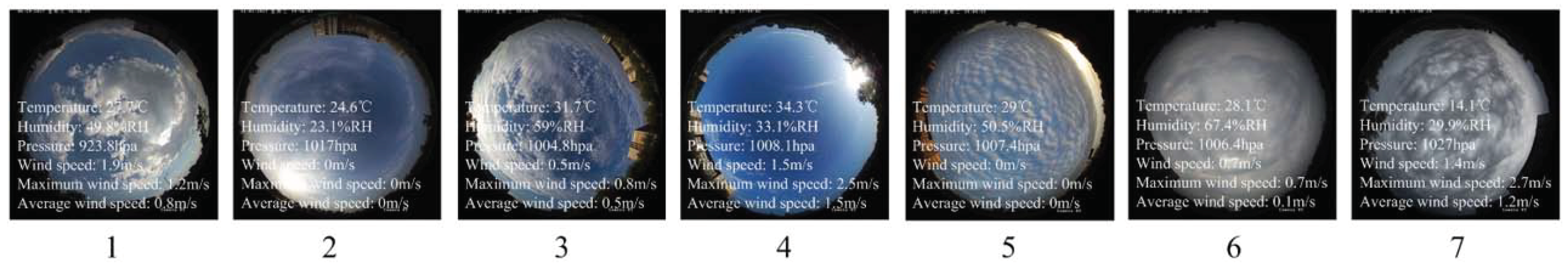
The MGC dataset collected in China mainly contains two kinds of ground-based cloud information, i.e., the cloud images and the multimodal cloud information. The cloud images with the size of 1056 × 1056 are shot at different times by a sky camera with fisheye lens. The fisheye lens could provide a wide range observation of the sky conditions with the horizontal and vertical angles of 180 degrees. Meanwhile, the multimodal cloud information is collected by a weather station, including temperature, humidity, pressure, wind speed, maximum wind speed and average wind speed. Note that the maximum wind speed and average wind speed are computed over each minute. It is worth mentioning that the sky camera and the weather station work concurrently, and, accordingly, each cloud image corresponds to a set of multimodal data. The MGC is a very challenging dataset due to the large intra-class and small inter-class variations, and it contains a number of 3711 labeled cloud data. According to the International cloud classification system criteria published in the World Meteorological Organization (WMO), and the visual similarity in practice, the sky conditions are divided into seven classes: cumulus, cirrus and cirrostratus, cirrocumulus and altocumulus, clear sky, stratocumulus, stratus and altostratus, cumulonimbus and nimbostratus. Besides, it should be noted that cloud images with cloudiness no more than 10% belong to clear sky. The number of cloud samples in each class is diverse from each other, and the detailed numbers are summarized in
Table 2. Herein, the Arabic numerals from 1 to 7 denote the labels of cloud classes.
Figure 3 exhibits some cloud samples from each class, and the multimodal information is embedded in the corresponding cloud image.
The MGC dataset is randomly split into training set and test set. The training set contains two-thirds of the cloud samples from each class and the test set is grouped by the remaining ones from each class. The split process is conducted 10 times independently, and the average accuracy over these 10 random splits is treated as the final ground-based cloud classification accuracy. For the sake of fair comparison, all the experiments follow the same experimental setup.
3.2. Baselines
The following seven baselines are presented to prove the validness of the proposed JFCNN.
(1) BoW [
43] model: The bag-of-words (BoW) model is a representative approach to describe images. We first extract the SIFT features in a dense manner. Then, we utilize
K-means algorithm to learn the dictionary. In our experiments, the dictionary contains 1024 codewords. As a result, each cloud image is expressed in the form of a 1024-dimensional histogram.
(2) PBoW [
44] model: The pyramid BoW (PBoW) model is obtained by incorporating the BoW model with the spatial pyramid (SP). The PBoW model could learn fine-grained information of cloud images in different spatial levels. The level number of SP for each cloud image is set to 3. Concretely, each cloud image has 1, 4, and 16 cells in the three levels, respectively. Thus, each cloud image is made up of 21 cells. We utilize the BoW model to represent each cell as a 1024-dimensional histogram, resulting in a 21504-dimensional feature vector for each cloud image.
(3) LBP [
45]: The local binary pattern (LBP) is a widely-used texture descriptor, which is robust to monotonic gray-scale changes caused by illumination variations. In our experiments, the uniform invariant LBP is applied to represent the ground-based cloud visual features. There are two important parameters
P and
R in LBP, where
P is sampling points number involved in a circle and
R is the circle radius. The ratio between
P and
R is fixed to 8:1 with the circle radius 1, 2 and 3, respectively. Then, the cloud representations from the three different conditions are grouped in a serial fashion. Hence, each cloud image is represented with a 54-dimensional vector.
(4) CLBP [
46]. The completed LBP (CLBP) is evolved from LBP and developed for texture classification. In CLBP, a local region is represented by its center pixel, and the local differences of signs and magnitudes. These three components are combined in joint distribution form to obtain the cloud representation. The parameters
P and
R follow the same settings in LBP. Then, the three scales are gathered into one feature vector by concatenating with the dimensions of 2200.
(5) PBoW + CLBP. The PBoW is the learning-based descriptor and CLBP is the hand-crafted descriptor. We concatenate them to obtain a 23704-dimensional feature vector for each cloud image.
(6) MMI. The multimodal information (MMI) forms a vector , where indicate the temperature, humidity, pressure, wind speed, maximum wind speed and average wind speed, respectively. In our experiments, we normalize the number ranges of the multimodal data into , and treat it as the ground-based cloud representation.
(7) Deep features. For extracting deep visual features, we remove the multimodal subnetwork and the joint fusion layer in the JFCNN. We denote this deep visual feature as V_DF which is a 2048-dimensional vector. To learn deep multimodal features, we remove the vision subnetwork and the joint fusion layer in the JFCNN. We denote the deep moltimodal feature as M_DF which is a 2048-dimensional vector.
For fair comparison, the above-mentioned baselines utilize the same training and test sets as the proposed JFCNN. In addition, the support vector machine (SVM) with radial basis function (RBF) kernel is used as the classifier for all methods. All the features are normalized by -norm before and after integration or before they are fed into the SVM classifier.
3.3. Comparison Results and Discussion
In this subsection, we first prove the effectiveness of the multimodal information and the joint fusion learning for ground-based cloud classification. The experimental results are shown in
Table 3. For better understanding, we first clarify the simplified forms listed in the table. MMI indicates the six-dimensional feature vector which directly concatenates six kinds of multimodal information of the ground-based cloud. M_DF denotes extracting the deep multimodal features from the separately learned multimodal network where we remove the vision subnetwork and the joint fusion layer in the JFCNN. Similarly, V_DF is the extracted deep visual features from the separately learned vision network where we remove the multimodal subnetwork and the joint fusion layer in the JFCNN. V_JFCNN, M_JFCNN and J_JFCNN indicate the outputs of vision subnetwork, multimodal subnetwork and the joint learning layer of JFCNN, respectively. JFCNN represent the weighted concatenation of V_JFCNN and M_JFCNN as shown in Equation (
5). Note that “+” denotes concatenating two feature vectors. For example, V_DF + MMI indicates concatenating V_DF and MMI, and so do V_JFCNN + MMI, and V_DF + M_DF.
In general, the compared methods are categorized into four parts, i.e., individual multimodal representations (MMI, M_DF and M_JFCNN), individual visual representations (V_DF and V_JFCNN), the integration of learned visual features and MMI (V_DF + MMI and V_JFCNN + MMI), and the integration of both learned visual features and learned multimodal features (V_DF + M_DF, JFCNN and J_JFCNN).
Several conclusions can be drawn from
Table 3. First, the proposed JFCNN achieves the best result of 93.37%. Second, the classification accuracy of MMI is 75.42%, which demonstrates the potential for ground-based cloud classification. It is because the MMI is only a six-dimensional vector and without any transformation, while the other methods are at least 2048-dimensional vectors and with learning process.
Third, the integration feature representations (V_DF + MMI, V_JFCNN + MMI, V_DF + M_DF and JFCNN) show better results than any of the individual feature representations (MMI, M_DF, M_JFCNN, V_DF and V_JFCNN). Moreover, the integration of both learned features (V_DF + M_DF and JFCNN) performs better than just learning the visual features (V_DF + MMI and V_JFCNN + MMI). It is because the integrated feature vectors could combine the complementary information of the two kinds of features and the integration of both learned features have more discriminability.
Fourth, the jointly learned features overshadow the separately learned features. Concretely, V_JFCNN and M_JFCNN exceed V_DF and M_DF at a percentage of 1.69 and 5.74, respectively. Moreover, the proposed JFCNN outperforms V_DF + M_DF. This is because the joint learning can take into consideration the consistency and complementary information between the two kinds of features and their relative importance for classification task. However, the V_DF + M_DF, which separately learns the features, has not thoroughly investigated the relationship between the visual features and the multimodal information.
To demonstrate the effectiveness of the proposed feature extraction (or fusion) method, we compare it with the end-to-end based methods. The comparison results are listed in
Table 4. Note that Accuracy 1 corresponds to the proposed methods, and Accuracy 2 corresponds to the end-to-end based methods. Herein, the end-to-end based cloud classification for JFCNN refers to J_JFCNN. In the table, we can see that the results in Accuracy 1 are all better than those in Accuracy 2. This demonstrates the effectiveness of the proposed feature extraction and fusion strategy.
Then, to evaluate the robustness of the proposed JFCNN, we enumerate a potential alternative structure for comparison with the proposed architecture. Specifically, after the average pooling layer in the vision subnetwork, we add a fully connected layer with 64, 128, 256 and 512 neurons, respectively. Accordingly, the outputs of the multimodal subnetwork are 64, 128, 256, 512 dimensions, respectively. Thereby, the input dimensions of the joint fusion layer are reduced. The comparison results shown in
Table 5 are satisfactory. However, the comparison between
Table 3 and
Table 5 demonstrates that the proposed JFCNN has an advantage over the modified architecture.
Moreover, we conduct an experiment to analyze the classification performance under different cloud sample numbers. Concretely, we utilize 1/4 (618), 1/3 (824), 1/2 (1237) and all the samples (2474) in the training set to train JFCNN, respectively. The comparison results are presented in
Table 6. As shown, using more samples leads to higher classification accuracy.
Next, we compare V_JFCNN and V_DF with some representative visual feaetures, and the results are listed in
Table 7. In
Table 7, we can see that V_JFCNN and V_DF obtain better results than other shallow visual features. Especially, the gain classification accuracies for V_JFCNN and V_DF are 12.15% and 10.46%, respectively, better than PBoW + CLBP which is a combination of learning-based feature (PBoW) and hand-crafted feature (CLBP). The improvements of the V_JFCNN and V_DF are reasonable as they are CNN-based features. The deep architecture of CNNs forces the raw cloud data through a series of highly nonlinear transformations, and therefore enables the extracted features to be held with high-level cloud semantic information.
Finally, we evaluate the classification performances of the multimodal information integration for different methods, and
Table 8 lists the classification results. In
Table 8, we can see that the proposed JFCNN significantly boosts the performance and the classification accuracy achieves up to 93.37%. The promising result owes to the multimodal information integration and the joint fusion learning strategy. The comparison between
Table 7 and
Table 8 shows that, with integrating MMI, the classification accuracies in the latter gain competitive edge. This indicates that the multimodal cloud information is beneficial for the ground-based cloud classification once again.
The improvement of the proposed JFCNN is quite reasonable. The cloud images are usually with very large intra-class and small inter-class variations, due to environmental influences of illumination, occlusion and deformation. A more powerful tool is required to obtain a completed cloud information and then we employ the weather station to collect the multimodal information. In the meantime, the proposed JFCNN could jointly learn the cloud visual information and the multimodal information and extract discriminative features for ground-based cloud data. Accordingly, we can obtain more accurate cloud representations and make a significant improvement of the classification accuracy.
3.4. Parameter Analysis
There are two important parameters,
and
, which control the significance of the multimodal information in Equation (
1) and Equation (
5), respectively. Appropriate
and
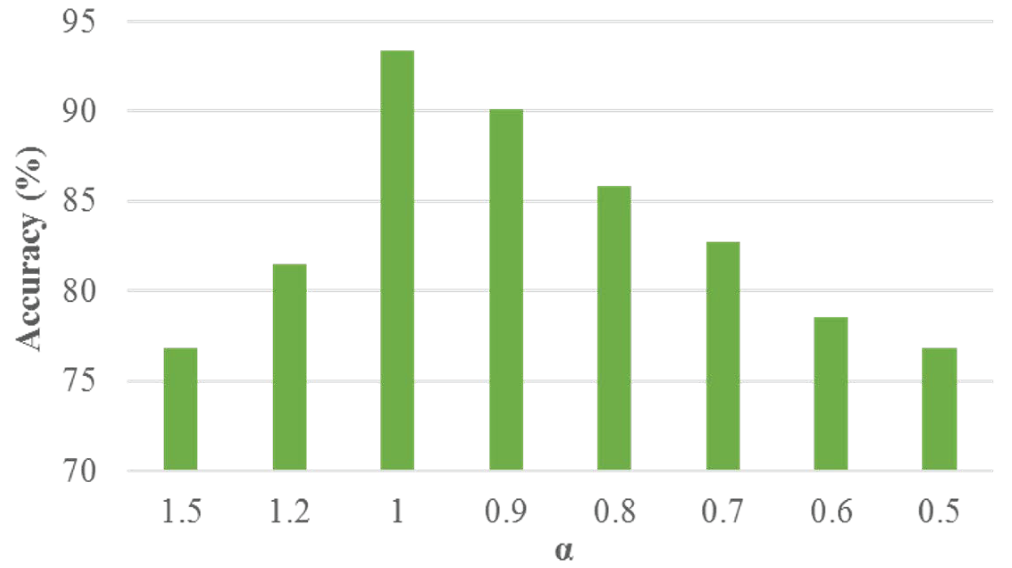
settings can optimize the classification results. We first evaluate the performance of
by changing its value for adjusting the significance of
in joint learning. The comparison results of different
settings are illustrated in
Figure 4. In the figure, we can see that, when
is set to 1, the best classification accuracy is obtained. Then, we evaluate the performance of
by tuning its value for balancing the significance of
in feature fusion. The comparison results of different
settings are illustrated in
Figure 5. In
Figure 5, we can see that, when
is set to 0.9, the best classification accuracy is obtained. This indicates that such
setting can well embody the significance of the multimodal features in the feature fusion stage.
We also evaluate the classification results under different drop rates in the dropout layer of JFCNN. The drop rates are set to 0.2, 0.3, 0.4, 0.5, 0.6, 0.7, 0.8 and 0.9, respectively, and the comparison results are listed in
Table 9. The results show that the classification accuracy with the drop rate of 0.9 is superior to other conditions.


