Article

Applying High-Resolution Imagery to Evaluate Restoration-Induced Changes in Stream Condition, Missouri River Headwaters Basin, Montana

by
Melanie K. Vanderhoof
* and
Clifton Burt
U.S. Geological Survey, Geosciences and Environmental Change Science Center, P.O. Box 25046, DFC, MS980, Denver, CO 80225, USA
*
Author to whom correspondence should be addressed.
Remote Sens. 2018, 10(6), 913; https://doi.org/10.3390/rs10060913
Submission received: 13 April 2018 / Revised: 1 June 2018 / Accepted: 7 June 2018 / Published: 9 June 2018

Abstract

:
Degradation of streams and associated riparian habitat across the Missouri River Headwaters Basin has motivated several stream restoration projects across the watershed. Many of these projects install a series of beaver dam analogues (BDAs) to aggrade incised streams, elevate local water tables, and create natural surface water storage by reconnecting streams with their floodplains. Satellite imagery can provide a spatially continuous mechanism to monitor the effects of these in-stream structures on stream surface area. However, remote sensing-based approaches to map narrow (e.g., <5 m wide) linear features such as streams have been under-developed relative to efforts to map other types of aquatic systems, such as wetlands or lakes. We mapped pre- and post-restoration (one to three years post-restoration) stream surface area and riparian greenness at four stream restoration sites using Worldview-2 and 3 images as well as a QuickBird-2 image. We found that panchromatic brightness and eCognition-based outputs (0.5 m resolution) provided high-accuracy maps of stream surface area (overall accuracy ranged from 91% to 99%) for streams as narrow as 1.5 m wide. Using image pairs, we were able to document increases in stream surface area immediately upstream of BDAs as well as increases in stream surface area along the restoration reach at Robb Creek, Alkali Creek and Long Creek (South). Although Long Creek (North) did not show a net increase in stream surface area along the restoration reach, we did observe an increase in riparian greenness, suggesting increased water retention adjacent to the stream. As high-resolution imagery becomes more widely collected and available, improvements in our ability to provide spatially continuous monitoring of stream systems can effectively complement more traditional field-based and gage-based datasets to inform watershed management.

Graphical Abstract

1. Introduction

Remotely sensed imagery has been widely applied to characterize variability in surface-water extent across space and time [1,2]. The spatial resolution (≥30 m) of commonly used sources of imagery (e.g., Landsat, MODIS, AVHRR), however, has limited our ability to remotely monitor river systems, except for large rivers (e.g., >40 m wide) [3] or rivers under flood conditions [4,5,6,7]. Yet remote monitoring of the spatial distribution of river stage and condition has several applications including enhancing our ability to predict and monitor flood events, informing the source and distribution of flow to downstream gaged points, helping monitor ungaged watersheds, predicting carbon dioxide emissions, and informing river management [8,9,10,11]. The rapidly increasing availability of multispectral, high-resolution imagery (≤5 m resolution, Dove, RapidEye (Planet, San Francisco, CA, USA), Worldview-2, 3 (DigitalGlobe, Westminster, CO, USA)) provides increased opportunity to potentially monitor river systems across diverse watershed sizes and flow conditions.
Multiple sources of fine resolution imagery have been applied to aquatic systems. LiDAR [12,13] and synthetic aperture radar (SAR) imagery have been successfully used to map surface water and can be preferable in forested environments or during storm events under cloud cover [14,15,16]. Multispectral, high-resolution imagery has also been used effectively to map surface water [17,18]. Riverscape units including the active channel have primarily been mapped by digitizing very high-resolution multispectral satellite imagery or aerial imagery [19,20,21] or by applying geographical object-based image analysis (GEOBIA) methods [11,22,23]. A GEOBIA approach segments an image into homogenous objects prior to object classification. Such an approach can help account for the greater within-class spectral variability that can occur with high-resolution imagery, relative to moderate-resolution imagery [18]. In general, however, efforts to remotely monitor narrow, linear water features, such as rivers and streams, have lagged behind efforts to remotely monitor lakes and wetlands [24,25].
The Upper Missouri River Headwaters Basin in southwestern Montana faces increasingly uncertain water supplies attributable to high water demand for agricultural irrigation [26,27] and public water supply [28,29]. In addition, shifts in the timing of runoff and peak streamflow are predicted with increasing amounts of winter precipitation and a declining snowpack related to climate change [30,31,32]. Societal water demands as well as climate-induced shifts in streamflow can threaten habitat critical for fish and aquatic species [33,34]. These risks have raised interest in increasing the capacity of streams to respond to extreme events [35,36,37]. One approach that is growing in popularity is to slow runoff, absorb excess floodwater, and encourage groundwater recharge by enhancing natural water storage in stream channels, riparian areas, and floodplains [38,39]. One way to create natural water storage is using in-stream, channel spanning structures called beaver dam analogues (BDAs) [40,41,42]. Over time BDAs have been shown to slow water flow, encourage channel stability and riparian vegetation, activate side channels, and improve water quality and fish habitat [40,41,43]. Installing BDAs along a reach of stream can potentially increase spring overbank flow and elevate riparian water tables [43]. If water is a limiting factor in the riverscape, elevating near-surface soil moisture along stream channels can encourage riparian vegetation [44,45]. Depending on channel shape and river stage, slowing the flow of water can increase the stream surface area through ponding and temporary flooding [38,45]. Downstream from beaver dams, channels are more likely to be stable, with lower sediment loads and a lower range of stream discharge [45]. Although the installation of BDAs is becoming relatively common, analyses that evaluate their impact are limited. Most studies to date have focused on the impact of actual beaver dams that differ from BDAs in the magnitude of change and maintenance activity. In this study, we tested how multispectral high-resolution imagery can be used to monitor stream condition along four stream reaches in the Upper Missouri Headwaters Basin, and how pairs of images can potentially be used to monitor BDA stream restoration projects. Our research questions included:
  • What methodological approaches are most effective to map stream surface area using multispectral high-resolution imagery? And,
  • How can image pairs (e.g., pre- and post-restoration) be used to monitor changes in stream surface area and riparian greenness?

2. Methods

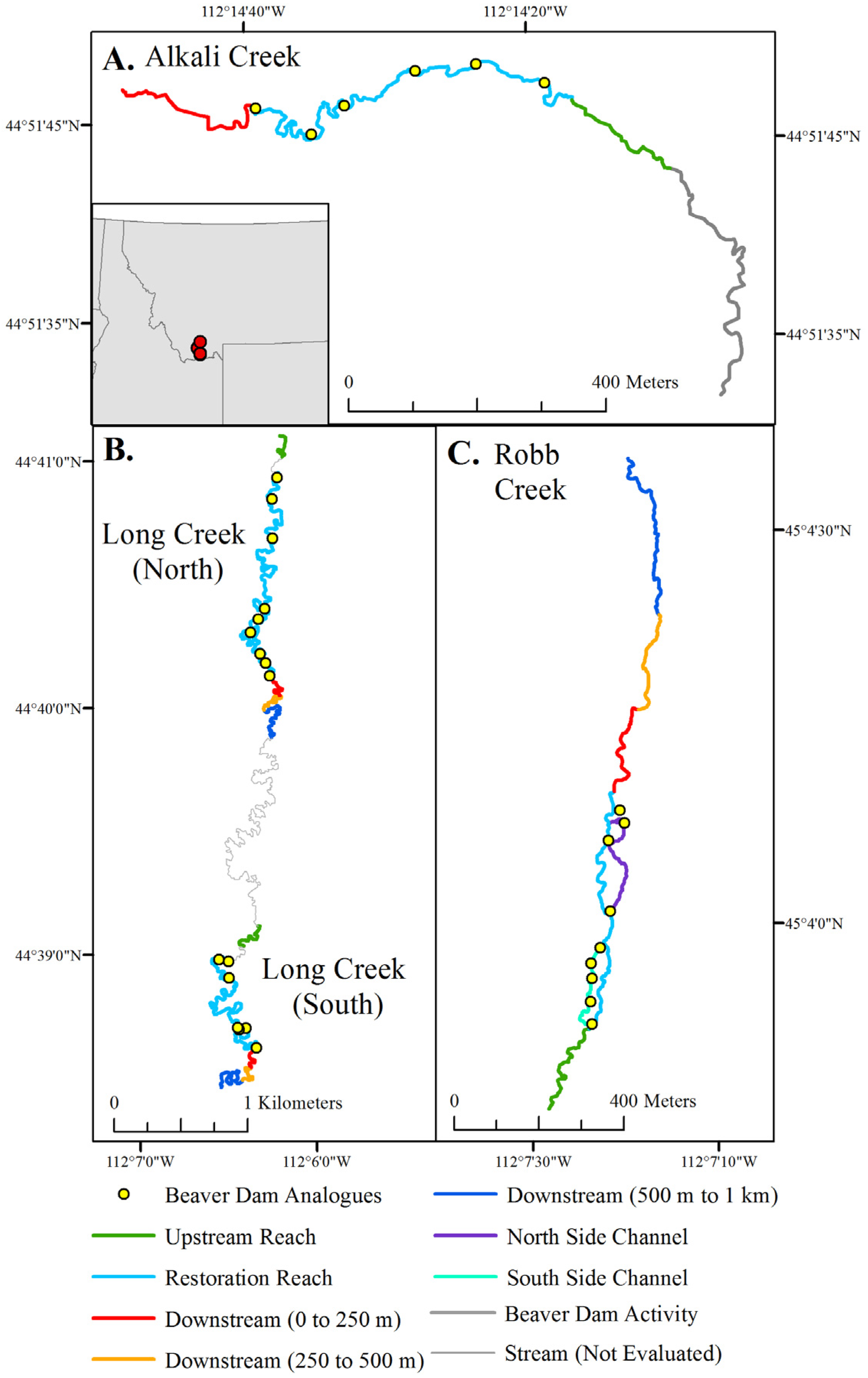
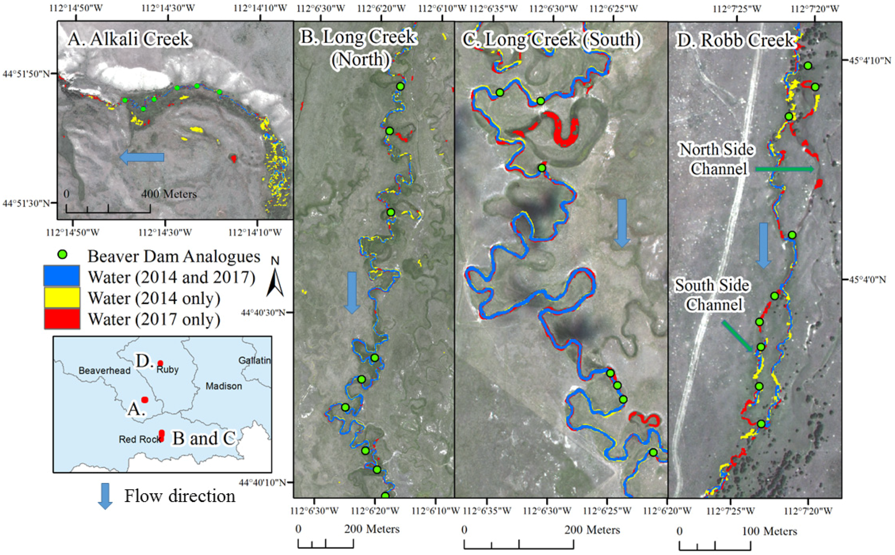
2.1. Study Area and Restoration Activities

The four stream sites examined in this study occur within the Upper Missouri Headwaters Basin in southwest Montana (Figure 1). Annual precipitation across the Headwaters Basin averages 565 mm yr−1, while the annual temperature maximum and minimum average 10 °C and −3 °C, respectively (1981–2010) [46]. Across the basin herbaceous vegetation (35%) and shrub/scrub (20%) dominate the large river valleys while evergreen forest dominates the higher elevations (35%) [47]. Two restoration sites occurred along reaches separated by 4.8 stream km in Long Creek (Figure 1), which flows south into the Red Rock River in the Red Rock River Hydrological Unit (Red Rock HUC8). Land cover adjacent to Long Creek is dominated by herbaceous vegetation, shrub/scrub, and emergent herbaceous wetlands [47]. The third restoration site occurred along Alkali Creek, which flows northwest into Blacktail Deer Creek in the Beaverhead HUC8. This site showed evidence of beaver activity just upstream from the restoration site. The fourth restoration site occurred along Robb Creek that flows north into the Ruby River (Ruby River HUC8). Land cover adjacent to both Alkali Creek and Robb Creek is dominated by herbaceous vegetation and shrub/scrub habitat [47].
All restoration activities were developed and completed by the Nature Conservancy. A series of BDAs were installed in stream reaches at each restoration site. The structures were created from wooden posts installed vertically into the streambed across the channel with willow branches woven between posts. The structures collect organic material and sediment behind them, building up the stream bed height, ponding water upstream from the structures, stabilizing the channel and increasing connectivity with its floodplain [48]. The BDAs were accompanied by willow plantings along the stream to stabilize banks and cattle exclusions at most of the sites [48]. The design is cost effective as no heavy equipment is used and the in-stream structures are designed to be temporary [49]. BDAs were installed in two reaches of Long Creek (9 BDAs on the north reach and 7 BDAs on the south reach), a reach of Alkali Creek (6 BDAs) and a reach of Robb Creek (12 BDAs) (Table 1). The goal of the restorations at the Long Creek and Alkali Creek sites was to aggrade the streambed, improving hydrologic connectivity between the stream channel and associated floodplains. Along Robb Creek, the BDAs were designed to encourage reactivation of abandoned side channels. The time since restoration ranged from one to three years across the sites (Table 1).

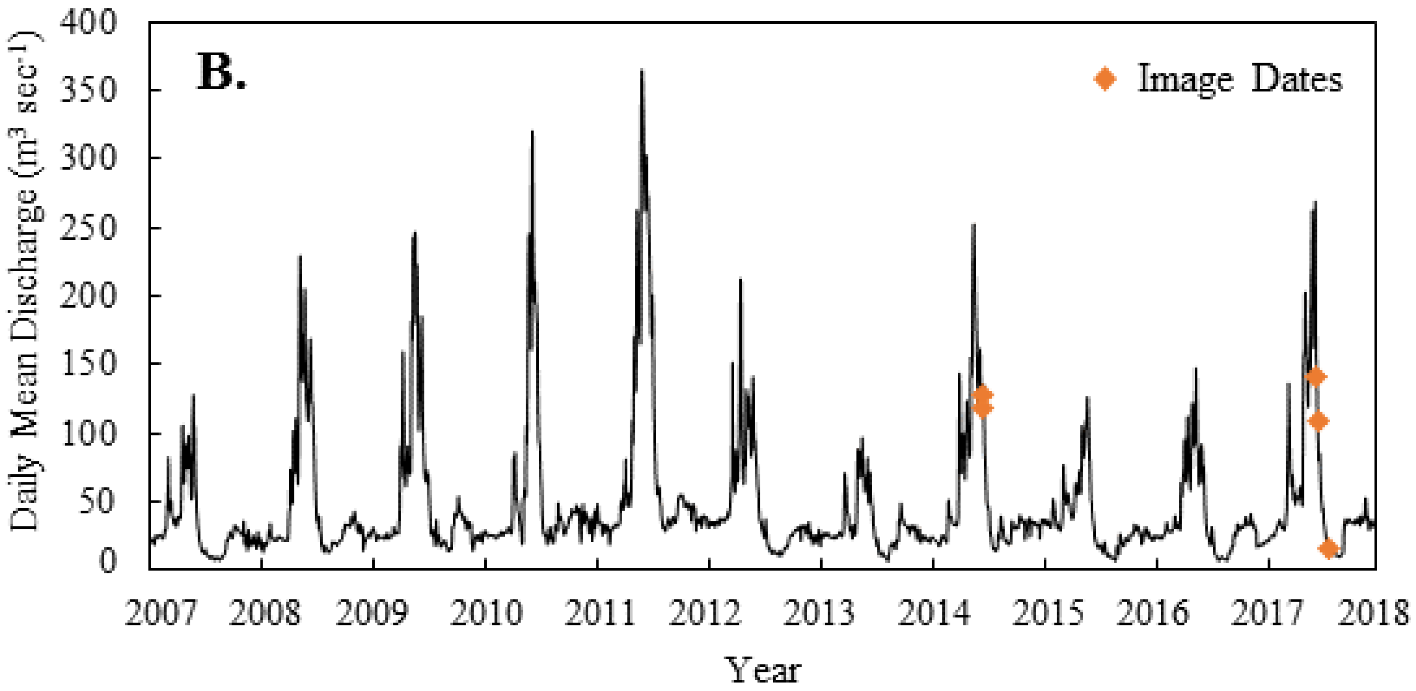
2.2. Image Acquisition and Preprocessing

A total of six high-resolution images (2 m resolution) were acquired from DigitalGlobe (Westminster, CO, USA) via the NextView license for this analysis. These images included one QuickBird-2 image, three Worldview-2 images, and two Worldview-3 images (Table 1). “Pre-restoration” conditions were represented by images acquired during summer 2014, while “post-restoration” conditions were represented by images acquired during summer 2017. Using historical (1895–2017) Palmer Hydrological Drought Index (PHDI) values, we found that the pre- and post-restoration image dates represented similar historical wetness conditions (37.6% relative to 41.8% PHDI); however, 2013, the year prior to the pre-restoration images experienced a drought which may have influenced stream conditions in 2014 (Figure 2). We also compared the stream discharge values on the date the image was collected using a USGS stream gage downstream from the four restoration sites (Jefferson River, USGS Gage #06026500) (Figure 1). Discharge was reasonably similar between the image dates (10% higher post-restoration for the Long Creek image dates and 8% lower post-restoration for the Robb Creek image dates), for all sites except Alkali Stream. The post-restoration image at this site was collected in August when discharge was much lower relative to the early summer period (Figure 2). We converted the image (processing Level 1) pixel values from Digital Numbers to top-of-atmosphere reflectance in PCI Geomatica. For each image the panchromatic and multispectral bands were orthorectified together using PCI Geomatica’s 2014 OrthoEngine. National Agricultural Imagery Program (NAIP) images (1 m resolution) were used as reference images (Long Creek and Robb Creek—22 October 2015, Alkali Creek—3 August 2013) together with the U.S. Geological Survey’s 10 m National Elevation Dataset (NED) [50]. Images were pan-sharpened to 50 cm resolution using PCI Geomatica’s PANSHARP2 tool [51]. The panchromatic band width for QuickBird-2 extends across all four of the multispectral bands (blue, green, red, NIR); however, the panchromatic band for Worldview-2 and Worldview-3 extends across only five of the eight spectral bands (excludes the coastal band, NIR1 and NIR2 bands). Prior work has shown that applying pan-sharpening methods to bands outside of the panchromatic range can distort the values in these bands [52]. To account for this, we pan-sharpened only the bands overlapping the panchromatic band using the PANSHARP2 tool. Bands outside of the panchromatic band range were resampled to 50 cm resolution using cubic convolution.

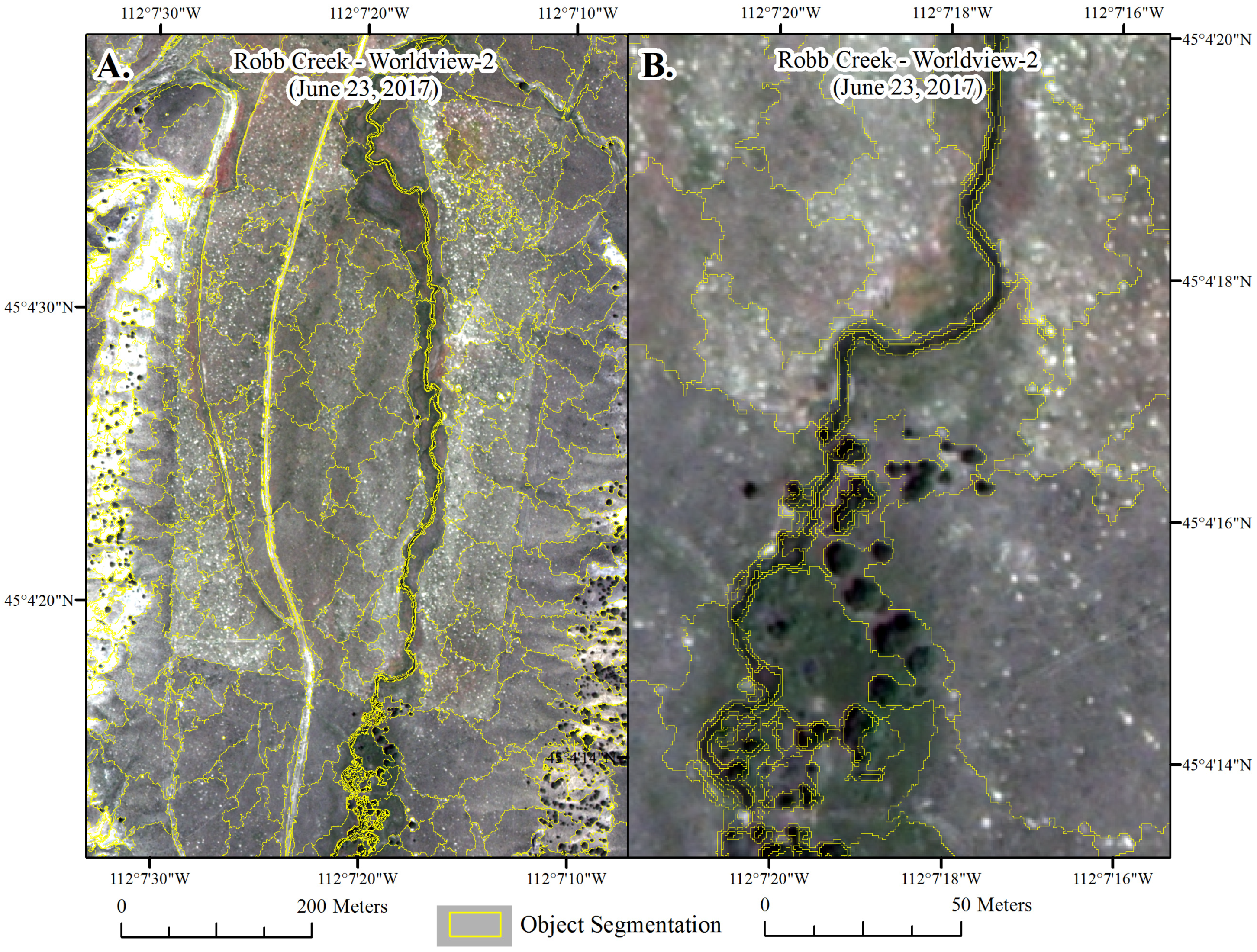
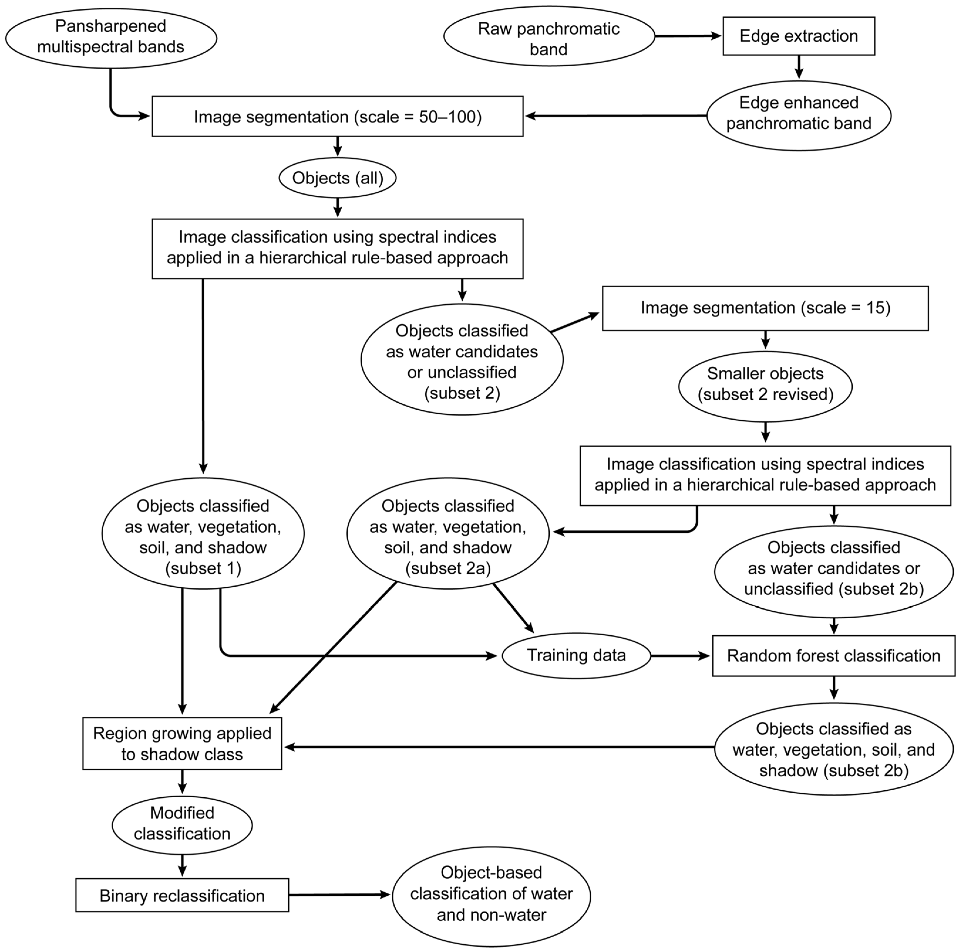
2.3. Object-Based Water Classification

We used the software eCognition (version 9.2.1, Trimble, Westminster, CO, USA) to process the high-resolution images into maps of surface-water extent. This software uses an object-oriented approach where an image is first segmented into objects representing meaningful features of the physical landscape, and the objects are then classified using user-defined rules and algorithms. Rules can be set in a hierarchical order as child rules under a parent process so that the ruleset can be automatically run in sequence. In this case, our objective was to segment, then classify objects into water and non-water where the objects of interest were the stream channels. Each pan-sharpened image was first clipped to the spatial area of interest, which included a minimum of 300 m stream length upstream from the restoration reach, the restoration reach and approximately 1 stream km downstream of the restored site (Figure 3). The stream length of the restoration reach (from the upstream to the downstream BDA) ranged from 830 m at Alkali Creek to 3.8 km at Long Creek (North) (Table 1).
To segment each image into objects we focused the segmentation along edges or sharp contrasts in the image. To do this we first modified the panchromatic band. Within eCognition, the Edge Extraction Lee Sigma filter was applied to the panchromatic band to create a (1) bright edge layer and (2) dark edge layer from the original image. The dark edge layer was then added to and the bright edge layer subtracted from an inverted version of the panchromatic band to enhance the edge contrasts along streams. The edge-enhanced panchromatic band was then used with the pan-sharpened blue, green, red, and near-infrared bands to guide the initial image segmentation (scale = 50–100). This approach focused segmentation along stream boundaries while segmenting the image at larger scales, where scale refers to the maximum allowable heterogeneity within an object. The larger scale was desired so that individual trees and tree shadows, which are spectrally similar to water, were segmented into larger objects that contained multiple trees, tree shadows, and intervening vegetation (Figure 4A). After the initial image segmentation, the objects were classified using spectral indices applied in a hierarchical rule-based approach. Our goal was to classify all objects as (1) water; (2) vegetation; (3) soil; or (4) shadow. Objects that were not spectrally similar enough to fit in any of these categories were classified temporarily as (1) water candidates (i.e., potentially water) or (2) unclassified. Objects classified as water candidates or unclassified using the rule-based approach were then re-segmented at a finer scale (scale = 15) to create smaller and more spectrally pure objects (Figure 4B).
Several spectral indices were included in our hierarchical rule-based approach (Table 2). Worldview-2 and 3 images (8 spectral bands) provide data from several bands not available in Landsat TM, ETM+ or QuickBird-2 including a coastal band, red edge band and two separate near infrared bands (NIR1 and NIR2), offering opportunities for unique band combinations [53]. The Normalized Difference Water Index (NDWI) [54] and the Worldview Water Index (WWI) [55] (Table 2) were used as the primary means to identify water objects. Objects were classified as water when either the NDWI or WWI object values were greater than zero. Objects were identified as vegetation when the objects had high Enhanced Vegetation Index (EVI) [56] values, using the coefficients generally adopted [57], or when they showed both a high Normalized Difference Vegetation Index (NDVI) [58] as well as a minimal difference between NDVI and EVI. Objects were classified as soil when the Green-Red Vegetation Index (GRVI) [59] value of objects was less than zero or where brightness values, derived from the panchromatic band, were high (Table 2). Shadow objects were identified using the normalized difference between the coastal band and blue band. For QuickBird-2 images in which the coastal band was not available this index was adapted to the normalized difference between the blue band and green band. A low brightness threshold, derived from the panchromatic band, was also used to identify shadowed areas. Finally, water candidates (i.e., potentially water) were identified using a series of indices. The rules to identify objects as water candidates were applied as child rules below the rules identifying objects as soil or vegetation. Indices used to identify water candidates included the NDWI using the coastal band instead of the green band [60] and panchromatic brightness, both of which were effective at identifying deeper water, as well as several novel band combinations including the Red Edge NDWI and Red Edge WWI both of which were helpful in mapping shallow water, particularly where sandy soils were visible below the water, and the Normalized Difference Coastal Red Edge Index (NDCREI) which was helpful in identifying turbid water. A list of the indices used, and the band combinations are shown in Table 2.
The hierarchical rule-based approach of classification was initially applied to all objects (scale = 50–100). For objects that were classified as water candidates or unclassified by the initial rule-based approach, these objects were re-segmented to create smaller, more homogenous objects (scale = 15) and the rule-based approach was re-applied to this subset of smaller objects. For objects classified as water candidates or unclassified after both rounds of rule-based classifications, we applied a Random Forest classifier to determine if these remaining objects were water, vegetation, soil, or shadow. The Random Forest classifier was trained using the objects already classified (either using scale = 50–100 or scale = 15) by the rule-based approach. Bootstrap iterations (n = 500) were run using all indices shown in Table 2, the individual band values, and the band standard deviations of the objects as independent variables.
Following the classification of all objects, in images that contained dense riparian vegetation with shadows, we applied the “grow region” algorithm to the shadow class in eCognition. This step reclassified the objects neighboring shadow objects as shadow candidates. We repeated the process as needed. More inclusive shadow thresholds were then applied to the shadow candidates and the objects were converted to shadow if they were within the thresholds. The object-based elliptic fit shape attribute was also used to classify individual tree shadows for trees that occurred near the stream. Although a similar segmentation and image classification approach was applied to all high-resolution images, as is common in the eCognition environment, a trial-and-error approach to segmentation and image classification was used [61] so that segmentation scale, index thresholds and rulesets were not identical across images. A flowchart showing our eCognition methods from image segmentation to an output of water and non-water is shown in Figure 5.

2.4. Pixel-Based Water Classification

Because a GEOBIA approach can be time-intensive and site specific, we were interested in comparing the performance of eCognition outputs with outputs producing using simplistic, single, spectral index thresholds. Using the pan-sharpened TOA reflectance values, we calculated the (1) NDWI [54]; (2) WWI [55]; and (3) the panchromatic brightness value. Brightness was calculated as the pixel value of the panchromatic band, a grayscale image of portions of the electromagnetic spectrum (Worldview-2, 3 (450–800 nm) and QuickBird-2 (450–900 nm)) (e.g., [62]). These three indices were selected as they were most prominently used to identify water objects in the eCognition image processing approach. The spectral index values of the validation points, described in Section 2.5, were used to guide the threshold selection. The rasters were thresholded to water and non-water using the maximum Youden’s index, which maximizes the difference between the true positive rate and the false positive rate from the ROC curve and provides an optimal threshold independent from class prevalence [63,64]. The Youden’s Index optimal threshold and corresponding AUC were calculated for each of the pixel-based outputs.

2.5. Stream Surface Area Validation

At each of the four sites, a stream line was manually delineated along each stream reach. The stream line was buffered (above and below the streamline, 1 m, 1.5 m, 1.8 m, 0.75 m for Alkali Creek, Long Creek (North), Long Creek (South), and Robb Creek, respectively) so that the total buffered area represented the average stream width. Points were randomly selected within the buffered stream area to represent water points (n = 200). The stream line was then buffered by 50 m and 200 points were randomly selected within the buffered area to represent non-water points. The 400 validation points per image were visually inspected using the raw pan-sharpened image to confirm status (water or non-water). Accuracy metrics calculated included overall accuracy, omission error, commission error, Dice coefficient, and relative bias. Omission and commission errors were calculated for the category of water. The Dice coefficient is the conditional probability that if one classifier (product or reference data) identifies a pixel as water, the other one will as well, integrating errors of omission and commission [65,66]. The relative bias provides the proportion that water is underestimated (negative bias) or overestimated (positive bias). Accuracy metrics were calculated for each of the pixel-based and object-based stream surface area outputs and presented by site, year, and methodology.

2.6. Changes in Stream Surface Area

To evaluate changes in stream surface area, our goal was to select the most accurate pair of stream surface area maps per site. This was determined using both the accuracy statistics as well as a visual assessment of quality. For Long Creek (North) and Long Creek (South), we used the panchromatic brightness output (97.4 and 98.4% overall accuracy, respectively when averaged across the two years, Table 3). For Robb Creek, we used the eCognition outputs (96.6% overall accuracy, averaged across the two years, Table 3), and for Alkali Creek, we merged the eCognition outputs with the panchromatic brightness outputs so that if water was identified by either output it was included as water. This was necessary only for Alkali Creek as the stream segment immediately downstream from the restoration was narrow (~1 to 1.5 m wide) and not adequately mapped using the eCognition output alone. Each output was edited manually to remove errors of commission. All outputs were converted to polygons and projected to WGS 1984 UTM zone 12 N prior to calculating area (m2) in ArcGIS 10.3 (ESRI, Redlands, CA, USA).
All surface water continuous with the stream centerline was included in stream surface area calculations, while waterbodies that were disconnected from the stream centerline were excluded from the stream surface area calculations. The total stream surface area was calculated for (1) the restoration reach, which extended from the upstream BDA structure to the most downstream BDA structure; (2) a reach extending upstream from the restoration reach (stream length of 300 m), and three reaches extending downstream from the restoration reach including; (3) a stream length of 0 m to 250 m downstream; (4) a stream length of 250 m to 500 m downstream; and (5) a stream length of 500 m to 1 km downstream from the restored reach. A schematic showing the distribution of these reaches at each site is shown in Figure 3. The stream length evaluated upstream and downstream from the restoration reach was limited by the extent of the pre- and post-restoration images. The same five reaches were used in analysis of the 2014 and 2017 images. At Robb Creek, the BDAs were aimed at reactivating side channels so each of the side channels were considered separately from the main channel (Figure 3). At Alkali Creek, beaver activity upstream from the restoration site influenced conditions in the upstream reach, so that the reach containing extensive beaver activity was analyzed separately (Figure 3). In addition, dense riparian vegetation approximately 300 m downstream from the restoration site in Alkali Creek limited our analysis of downstream area, so that results were presented only for a single downstream reach (0 m to 300 m) (Figure 3).
The challenge in evaluating the effects of restoration is to separate change attributable to natural variation (interannual, seasonal, event) from change attributable to the restoration activities. To accomplish this, we assumed that variability in hydro-climatic conditions would propagate similarly at the scale of adjacent or nearby stream reaches. Therefore, the ratio between the condition (e.g., amount of water, greenness) of an upstream reach and downstream reach at T1 should be equivalent to the ratio between the condition of the same upstream reach and same downstream reach at T2.
O   u p s t r e a m   r e a c h T 1 O   d o w n s t r e a m   r e a c h T 1 = O   u p s t r e a m   r e a c h T 2 E   d o w n s t r e a m   r e a c h T 2
where O refers to the observed value and E refers to the expected value. If we let the downstream reach represent the restoration reach, we can provide the values for the pre-restoration conditions (upstream and downstream reach values at T1) and the value for the upstream reach at T2 and solve for the “expected” value of the downstream reach (i.e., restoration reach) at T2. We can then use the observed downstream reach value at T2, to calculate the percent change from the expected value that we can attribute to the restoration activities:
C h a n g e   a t t r i b u t e d   t o   r e s t o r a t i o n   ( % ) = ( O   d o w n s t r e a m   r e a c h T 2 E   d o w n s t r e a m   r e a c h T 2 ) E   d o w n s t r e a m   r e a c h T 2 100
Calculating change as a function of the expected value can help account for variability between the images due to natural variability in climate and stream discharge. Although the outputs used to analyze changes in stream surface area tended to show high accuracy, if we assume that error induced by the methodology is random or consistent across the image extent, this approach also allowed us to take into account between-image variability in the accuracy of the mapped stream extent. We also recognize that changes to the restoration reach can potentially propagate upstream (e.g., [67]), possibly influencing the relationship between the upstream and downstream reaches; however, due to image extents we were limited in how far upstream we could document stream surface area necessitating the above assumptions.
In addition to calculating changes in stream surface area at a reach scale, we also calculated changes in stream width, inundated length, and changes to stream surface area just upstream from each BDA. To calculate changes in stream width, 20 points were randomly selected along the stream centerline within each site and reach and stream width was measured manually using the pan-sharpened raw imagery and averaged to obtain a single mean stream width per reach. The same points were used in both years. Inundated stream length was calculated as the percent of the stream centerline mapped as water. To quantify local changes in stream surface area induced by the structures, we calculated the stream surface area immediately upstream of each of the structures that showed a visually evident change (from 2014 to 2017) in stream width. Stream surface area was calculated from the classified (edited) stream surface area used to quantify reach-scale changes. The local change in stream surface area was presented as the change relative to pre-restoration stream surface area. The localized change was observed over a variable stream length distance, but the observed effect averaged 26 m of stream length upstream from the installed BDAs.

2.7. Changes in Riparian Condition

Riparian greenness was evaluated using three vegetation indices, NDVI, EVI and the Soil-Adjusted Vegetation Index (SAVI) [65]. Multiple indices were included because vegetation indices are sensitive to several conditions including canopy geometry (trees versus herbaceous vegetation), soil properties, sun position, and cloudiness [68,69,70]. While NDVI is the most commonly used vegetation index, EVI can help eliminate atmospheric noise, and SAVI reduces the influence of soil by including a soil adjustment factor (L) [56,68]. Changes in riparian greenness, averaged across the three indices, were then evaluated, (1) along the restoration reach (from the upstream BDA to the downstream BDA); (2) 0 m to 250 m downstream from the restoration reach; (3) 250 m to 500 m downstream from the restoration reach; and (4) 500 m to 1 km downstream from the restoration reach. At Robb Creek, the BDAs were designed to reactivate side channels so the side channels were considered separately from the main channel. We also tested how the effect changed as the buffer from the main channel increased from 10 m to 20 m from the channel centerline.
It was critical to control between-image differences in greenness not related to the restoration, therefore changes in greenness between the pre- and post-restoration riparian corridors were corrected using the difference in greenness across reference areas. Three reference polygons were selected at each site (ranging from 0.2 ha to 2.5 ha in size) representing: (1) herbaceous photosynthetic riparian vegetation upstream from the restoration site; (2) an upland patch dominated by photosynthetic grasses; and (3) an upland patch dominated by non-photosynthetic grasses. We avoided areas that appeared to show a difference in grazing intensity between the two image dates. The greenness values for each of the reference polygons were averaged to obtain a reference greenness value for each site and date. Because herbaceous vegetation is more sensitive to interannual change than riparian tree species, the reference polygons included a mix of riparian and upland vegetation samples. Additionally, because changes may have occurred for upstream vegetation in response to the restoration measures, we used a mix of riparian and non-riparian patches. Even at sites with willow plantings, short-term changes (one to three years) in riparian condition can be expected to primarily result from growth of herbaceous species, a change attributable to increased water availability in the shallow subsurface areas adjacent to the stream. The “reference greenness” values were seen as equivalent to the role of the upstream reach values when analyzing changes to stream surface area. The same analysis used to evaluate restoration effects on stream surface area above (Equations (1) and (2)) were applied here to evaluate restoration-induced changes to riparian condition.

3. Results

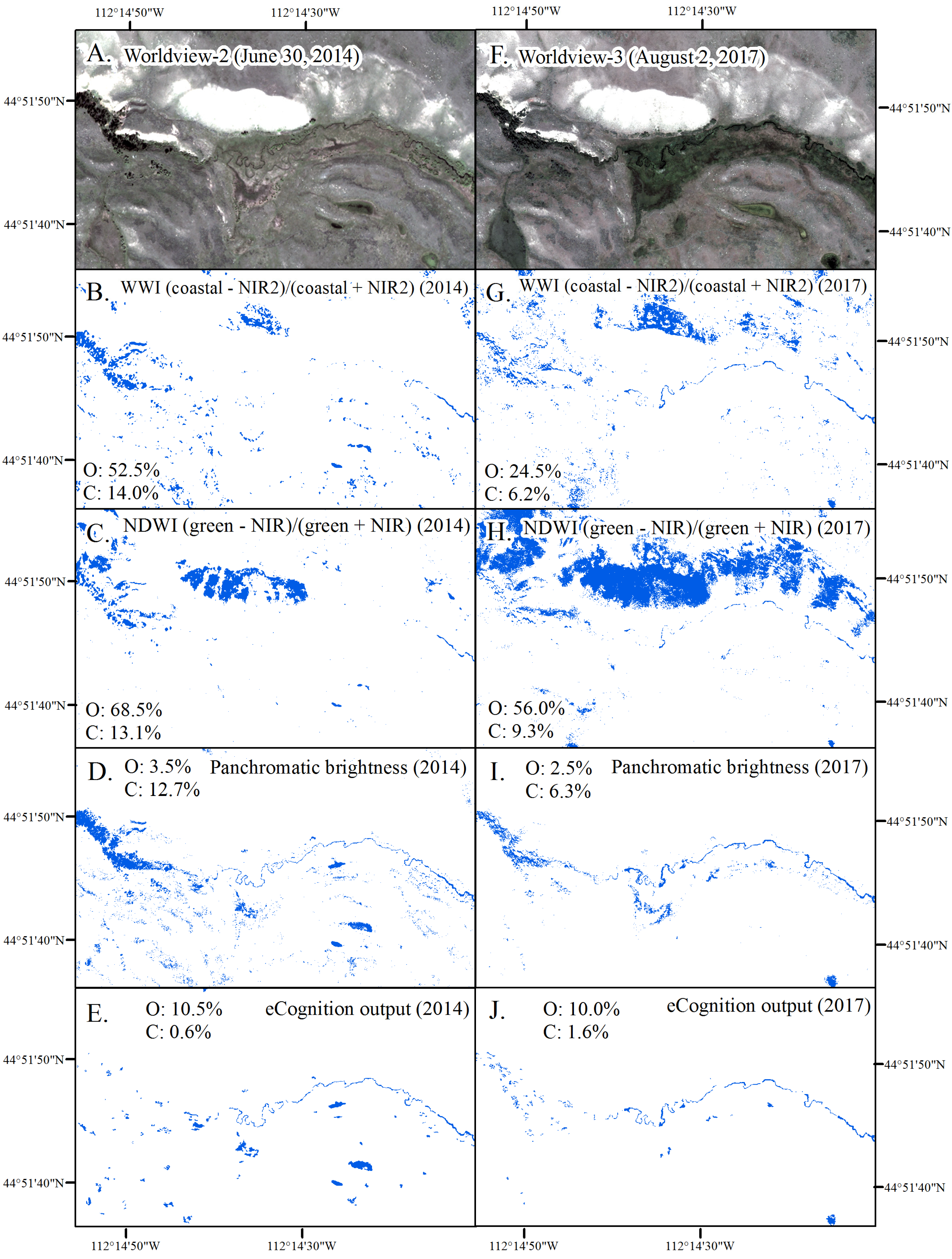
3.1. Accuracy of Stream Delineation Approaches

The accuracy of our estimates of stream surface area depended on both the stream width and the classification approach. Across all sites and classification approaches, the relative bias tended to be negative, indicating that the stream surface area, on average, was underestimated. Long Creek (South), which showed a stream width averaging 3 m to 3.5 m and Long Creek (North), which showed a stream width averaging 2.5 to 3.5 m wide, showed more consistent accuracy statistics across the approaches tested relative to the other two sites. The eCognition output and Panchromatic brightness consistently performed the best with errors of omission for water ranging from 2% to 6% and errors of commission ranging from 0.5% to 7%. In contrast, the NDWI tended to show higher errors of omission, with omission errors ranging from 7% to 37% and commission errors ranging from 1% to 5% (Table 3). Overall accuracy and dice coefficients were >95% except for NDWI outputs and one of the four WWI outputs (Table 3).
As stream width decreased at the Alkali Creek (averaged 1 m to 2.5 m) and Robb Creek (averaged 1.5 m to 2 m) sites, the accuracy of published indices (NDWI and WWI) was relatively poor. Using these indices errors of omission, for instance, ranged from 16% to 69% along the two streams. However, panchromatic brightness and eCognition outputs maintained relatively strong accuracy even as stream width decreased with errors of omission and commission across the two sites and years ranging from 3% to 11% and 2% to 13%, respectively, and the corresponding overall accuracy and Dice coefficient ranging from 91% to 97%.
It was also evident that classification accuracy for a given method can be inconsistent over time. Examples of this are shown in Figure 6, in which we can compare the outputs for each classification approach and year along the Alkali Creek site. Figure 6 also demonstrated that when surface water is a minority cover type across the image extent, an output can visually appear to be relatively noisy but statistically show a relatively low amount of calculated commission error. An example of this is the panchromatic brightness output for 2014 in which an error of commission of 13% created a visually “noisy” output. The visualized variability in the surface-water extent across methods justifies the need to analyze changes in stream surface area using the most accurate method possible and including a manual editing component as time allows so that uncertainty in surface-water extent does not obscure “true changes” in stream condition.

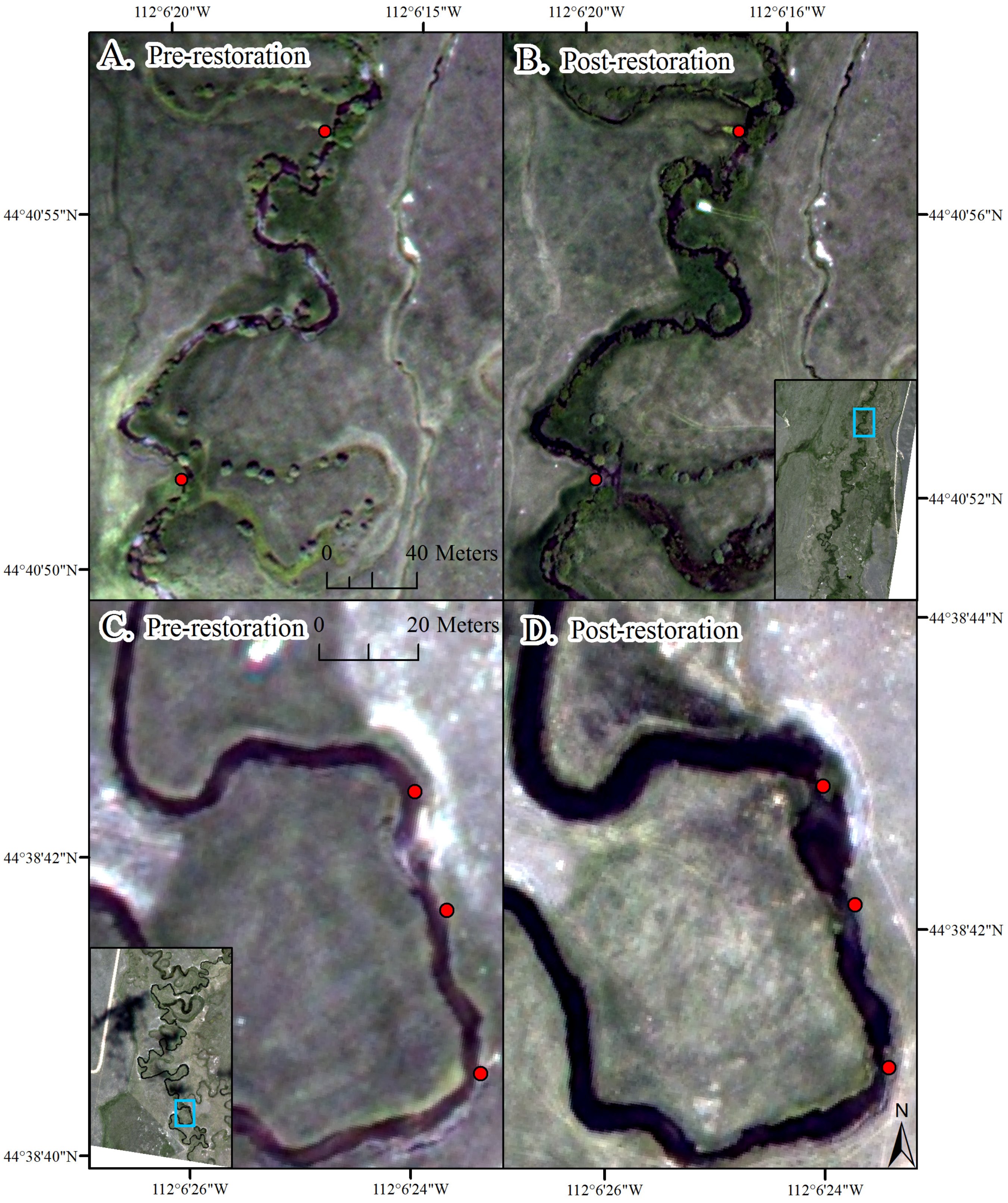
3.2. Changes to Stream Condition

The installation of BDAs resulted in proximal changes (e.g., increases in surface water immediately upstream from the in-stream structures) as well as changes at the scale of the restoration reach and downstream reaches. Increases in stream surface area immediately upstream from structures or in reactivated side channels were observed at all four sites. Increases in total stream surface area along the restoration reach were observed at three of the four sites, while a decrease in stream surface area downstream from the restoration reach was observed at all four sites (Table 4).
At Alkali Creek approximately one year post-restoration, we observed a net increase of 303 m2 in stream surface area immediately upstream from installed BDAs (Figure 7). This amount of water represented 19% of the total stream surface area along the restoration reach in 2017. After controlling for differences in stream surface area attributable to interannual variability, we observed a 25% increase in stream surface area attributable to the restoration activities, and a 30% decrease in stream surface area downstream from the restoration reach (Table 4). These changes in stream surface area were matched by corresponding changes in stream width (Table 4). A complicating factor at this site was that beaver activity was present from 200 m to 800 m upstream from the restoration reach. Upstream ponding resulting from natural beaver dams was substantial in the 2014 image but total stream surface water along the beaver impacted reach (200 m to 800 m upstream) decreased 74% by 2017 (Table 4, Figure 8A).
The goal of the restoration along Robb Creek was to reactivate two side channels. At approximately two years post-restoration, we observed a reactivation of the side channels that included a 78% increase in stream surface area along the northern side channel and a 356% increase in stream surface area along the southern side channel (Table 4, Figure 8). Correspondingly, we observed a 27% decrease in stream surface area along the main stream stem, and a decrease in stream surface area downstream from the restoration reach (0 m to 500 m downstream) (Table 4).
Long Creek (South) is 4.8 stream km downstream from Long Creek (North) and was the first restored of the four sites. At the time of the post-restoration image the site was approximately three years post-restoration. We observed a substantial amount of water stored upstream of many of the structures (net increase of water surface area of 747 m2) (Figure 9), which represented 6% of the total stream surface area along the restoration reach in 2017. We observed a 14% increase in stream surface area along the restoration reach and a corresponding decrease in stream surface area (−17% to −20%) from 0 m to 500 m downstream from the restoration reach (Table 4). Long Creek (North) at one-year post-restoration was the only site where we did not observe an increase in stream surface area along the restoration reach, but instead observed a minor decrease of 5% in stream surface area. We also observed the smallest increase in stream surface area upstream from the BDA structures (net increase of proximal water surface area of 171 m2), relative to the other sites evaluated (Figure 9). Similar to other sites, however, Long Creek (North) showed a decrease in stream surface area (−9% to −16%) through 1 km downstream from the restoration reach and an associated decrease in mean stream width (Table 4, Figure 8).

3.3. Changes to Riparian Condition

At each site, the spectral greenness index used (NDVI, EVI or SAVI) showed a relatively minor but inconsistent influence on the reported change in greenness, after controlling for between-year differences in greenness. EVI, for example, showed a higher percent change in greenness relative to NDVI and SAVI along Alkali Creek and Robb Creek, but not along the Long Creek sites (Table 5). However, we also found that the directionality of change to riparian condition post-restoration at each of the sites did not depend on the greenness index used. Increases in riparian greenness along the restoration reach were observed at three of the four sites, while changes to riparian greenness downstream from the restoration reach were less consistent.
Along Alkali Creek, we observed an average increase in greenness of 20% using a 10 m stream buffer, declining to a 15% increase using a 20 m stream buffer (Table 5). Although we had observed a decrease in stream surface area downstream from this restoration site, we found an increase in greenness that persisted through 1 km downstream from the restoration reach. Defining reference conditions required particular attention along Alkali Creek because the post-restoration image was late summer (August 2, 2017) when water is more limited. This is evident in the contrast observed in the NDVI between the riparian area and uplands in the 2017 Alkali Creek image (Figure 10). Along Robb Creek, minor increases in greenness were observed along the main stem and northern side channel (<5%), while a substantial green-up was observed along the southern side channel that showed an increase in greenness of 21% (Figure 10). The decrease in stream surface area observed downstream of this restoration site was found to co-occur with a decrease in greenness, which ranged from a 4% to 12% decrease in greenness through 1 km downstream of the restoration (Table 4). Although Long Creek (North) showed a minor decrease in stream surface area within the restoration reach, we observed an increase in greenness of 7 to 8% along the restoration reach and an increase in greenness of 13 to 15% just downstream of the restoration reach (0 to 250 m) (Figure 11). In contrast, while we observed clear changes in stream surface area along Long Creek (South), changes in greenness were minimal (<5% change) (Table 5, Figure 11).

4. Discussion

Long-term trends in the degradation of riparian and stream habitat are common across the western United States [71,72]. Satellite imagery has the potential to provide spatially continuous monitoring of stream extent and condition, which can complement point-based field efforts and stream gage data, and better inform stream management in response to degradation. However, only a limited number of studies have attempted to apply satellite imagery to streams, particularly smaller streams (<5 m wide). We found that pan-sharpened high-resolution imagery can be used to effectively monitor streams as narrow as 1.5 m wide. We tested sites where stream width was <1 m and found the results too poor to include. Panchromatic brightness consistently outperformed more established indices such as the NDWI. However, in experimenting with the classification of stream surface area we found that spectrally mixed portions of a stream can be more challenging to identify using this approach, for instance, portions of the stream showing high turbidity, high chlorophyll levels or bright sands can be missed using brightness alone. In addition, vegetation shadows, common in riparian areas, can be erroneously mapped as inundated areas, creating substantial errors of commission. Alternatively, while far more time consuming, a GEOBIA approach was able to greatly reduce errors of commission outside of the stream area by increasing object size with distance from stream and adding region growing to the shadow class within heavily shadowed riparian areas. While the index- and object-based approaches showed distinct advantages, we found that regardless of efforts accuracy results could be uneven across years. This is a major challenge in change detection analysis in which uneven accuracy over time, potentially attributable to differences in sensors, the off-nadir view angle, as well as the time of day that the image was collected or variability in local hydro-climatic conditions, can obscure change attributable to human-caused degradation or restoration [73]. We sought to minimize this source of error by (1) using only our most accurate outputs and further manually editing these outputs prior to analyzing changes in stream surface area; and (2) calculating the change as a function of the change from the expected value, therefore controlling, to the extent possible, for change due to image quality or variability in hydro-climatic conditions. This aspect of remote sensing change analysis, however, remains a challenge. Additionally, as the method that produced the highest overall accuracy varied also across sites, it was evident that the appropriate processing approach to minimize uneven error over time will vary across sites depending on the amount and type of riparian vegetation (herbaceous or tree), stream width, as well as water depth and clarity, a finding supported by others [74,75].
Improving techniques to map stream surface area with commercial high-resolution imagery offers opportunities to remotely monitor changes in key aspects of stream condition induced by flood or drought events, shifts in local land uses, or in-stream restoration activities. However, it is important to clarify that the stream data gleaned from a remote sensing analysis is intrinsically different from the data a hydrologist typically uses. For example, at the Alkali Stream site, differences in the seasonality of the image pair (June vs. August) meant that the downstream discharge in the Jefferson River was much lower at the August date relative to the June date (15 m3 s−1 compared to 127 m3 s−1); however, the stream surface area upstream from the restoration reach along Alkali Creek was only 3% less at the August date relative to the June date. This contrast clarifies that a remote sensing analysis is not necessarily capturing changes in stream discharge, which are better measured with stream gages, but instead providing a spatially continuous dataset of changes in stream surface area, specifically stream width and the creation or change to riparian wetlands, which could in turn, impact downstream stream discharge.
Relying on image pairs, however, or only two points in time, can limit our understanding regarding seasonally specific effects. For example, local stakeholders are interested in the effects of BDAs on streams not just after snowmelt, but in particular during the late summer period in which water availability can be limited [27,31]. Because very few DigitalGlobe images have been collected and archived across southwestern Montana we were restricted to the early summer period and were therefore unable to evaluate the impact of the BDAs during this late summer period. This limitation in image timing means we were unable to observe how changes in stream surface area or riparian condition documented near the start of the growing season influenced conditions near the end of the growing season. However, this limitation will likely be reduced in the near future. Sentinel-2 (10–20 m resolution), launched in June 2015, was too coarse for the streams evaluated, but in the future, could be used to regularly monitor the condition of rivers >10 m wide. CubeSats, such as those launched by Planet (San Francisco, CA, USA), also show high potential for improved monitoring of stream condition at more frequent intervals. Obstacles to the widespread application of CubeSats for monitoring stream condition, however, include the limited number of spectral bands (blue, green, red, near-infrared), the cost of Planet imagery, as well as challenges in calibrating reflectance and georeferencing between satellites e.g., [76]. As these technical obstacles are overcome, satellite imagery can be more commonly used to monitor streams in a spatially continuous manner.
We found separating the influence of weather relative to the influence of human-induced change particularly challenging in the riparian areas. Trends in riparian condition could be very sensitive to how reference conditions were defined. In part, this is because we might expect that the magnitude of interannual variability may be inconsistent across areas dominated by trees versus herbaceous vegetation. Additionally, reference areas can be influenced by forces of change independent of weather patterns such as variability in grazing intensity. The use of image pairs, and the time-frame at which the projects were considered (one to three years post-restoration), also limited our ability to evaluate the success of the activities with a lagged response, such as the tree planting effort, which takes more time to establish and can act to further influence riparian-stream interactions over time [44,77]. Riparian and wetland herbaceous species, however, can respond very quickly to changes in riparian soil moisture [71,77]. Therefore, changes in riparian greenness can be used to indirectly assess short-term changes to the stream hydrologic processes [77,78,79]. Because changes in riparian greenness were detected even when using a 20 m stream buffer, it may be possible to monitor riparian condition for streams <5 m wide using moderate resolution satellites, such as Landsat or Sentinel-2. As riparian trees grow larger and become more established, they can also impact our ability to monitor stream surface area. For instance, stream length at most sites was found to be <100% inundated, a finding that can be attributed to overhanging vegetation or hyporheic flow masking stream water.
Because our analysis relied on just two high-resolution images per site, we view this analysis as an example of the capabilities and potential of using high-resolution imagery to monitor stream condition and not a conclusion on the impact of specific restoration methods (e.g., BDAs, riparian planting) on streams. However, despite these concerns, we saw proximal evidence of increases in stream surface area upstream from structures at all four sites and evidence of either increases in stream surface area or riparian greenness along the restoration reach at all four sites. We also saw a decrease in stream surface area downstream from the restoration reach at all four sites. These findings suggest that the restoration activities have induced increases in instream water storage, at least during the early summer period. Uneven findings regarding the change induced by BDAs could be due to several factors including stream size, pre-restoration conditions [41], restoration goals, restoration installation (including extent and age), and site specifics, all of which can influence how a stream responds to change through time. However, these findings suggest that high-resolution imagery can provide a spatially continuous understanding of how narrow (<5 m wide) streams respond to restoration projects.

5. Conclusions

As high-resolution, multispectral imagery becomes more frequently collected and available, regular monitoring of stream surface area and condition in response to local or watershed-based changes will become increasingly feasible. However, mapping narrow, linear water features that are subject to rapid changes in water depth and turbidity may require approaches independent from those widely applied to map wetlands and lakes [1,2,80]. We found that utilizing bands unique to Worldview-2 and 3 in an eCognition framework can produce accurate results and minimal errors of commission down to a stream width of approximately 1.5 m. By comparing images pre- and post- restoration across multiple sites in the Upper Missouri River Headwaters Basin, we were able to quantify proximal and reach-scale changes in stream surface area and riparian greenness in response to the installation of multiple BDAs at each site. In general, the installation of BDAs appeared to create an increase in stream surface area immediately upstream from many of the structures. These proximal changes tended to result in reach-scale increases in stream surface area and riparian greenness along the restoration reach as well as decreases in stream surface area for reaches just downstream (through 500 m) from the restoration reach at most of the sites. The consistency of the directional changes to stream surface area across the sites, despite differing patterns in discharge lower in the watershed between-image pairs, suggests that we were able to account for hydro-climatic variability. Restoring degraded streams can positively influence in-stream habitat, water quality as well as water quantity across a watershed [34,37,38]. Monitoring the impacts of stream restoration projects, including resource-efficient structures such as BDAs, can improve and inform site selection and expectations for future stream restoration efforts.

Author Contributions

M.K.V. designed the study, performed the data analysis, and wrote the manuscript. C.B. led the image processing effort.

Acknowledgments

This project was funded by a U.S. EPA Region 8 grant, entitled “Building drought resiliency and watershed prioritization using natural water storage techniques” and through the associated interagency agreement (DW-014-92475401-0). This project was also supported by the USGS Land Resources, Land Change Science Program. All restoration actions were developed and implemented by the Nature Conservancy. We thank Tina Laidlaw and Ayn Schmit with U.S. EPA Region 8 as well as Laurie Alexander, Heather Golden, Jay Christensen, and Charles Lane with U.S. EPA, Office of Research and Development for their support and leadership in acquiring the funds and initial project development. We thank Nathan Korb of the Nature Conservancy and Jeff Burrell of the Wildlife Conservation Society for their invaluable help in site selection and knowledge of the field conditions, and Todd Hawbaker, Laurie Alexander, and the anonymous reviewers for their vital comments on earlier versions of the manuscript. Following publication, the data related to this publication will be published in the ScienceBase catalog (doi:10.5066/P9F9618G). Any use of trade, product, or firm names is for descriptive purposes only and does not imply endorsement by the U.S. Government.

Conflicts of Interest

The authors declare no conflicts of interest.

References

  1. Smith, L.C. Satellite remote sensing of river inundation area, stage, and discharge: A review. Hydrol. Process. 1997, 11, 1427–1439. [Google Scholar] [CrossRef]
  2. Alsdorf, D.E.; Rodriguez, E.; Lettenmaier, D.P. Measuring surface water from space. Rev. Geophys. 2007, 45. [Google Scholar] [CrossRef] [Green Version]
  3. Wang, J.J.; Lu, X.X.; Liew, S.C.; Zhou, Y. Retrieval of suspended sediment concentrations in large turbid rivers using Landsat ETM+: An example from the Yangtze River, China. Earth Surf. Process. Landf. 2009, 34, 1082–1092. [Google Scholar] [CrossRef]
  4. Wang, Y.; Colby, J.D.; Mulcahy, K.A. An efficient method for mapping flood extent in a coastal floodplain using Landsat TM and DEM data. Int. J. Remote Sens. 2002, 23, 3681–3696. [Google Scholar] [CrossRef]
  5. Qi, S.; Brown, D.G.; Tian, Q.; Jiang, L.; Zhao, T.; Bergen, K.M. Inundation extent and flood frequency mapping using Landsat imagery and Digital Elevation Models. GISci. Remote Sens. 2009, 46, 101–127. [Google Scholar] [CrossRef]
  6. Chen, Y.; Huang, C.; Ticchurst, C.; Merrin, L.; Thew, P. An evaluation of MODIS daily and 8-day composite products for floodplain and wetland inundation mapping. Wetlands 2013, 33, 823–835. [Google Scholar] [CrossRef]
  7. Ogilvie, A.; Belaud, G.; Belenne, C.; Bailly, J.S.; Bader, J.C.; Oleksiak, A.; Ferry, L.; Martin, D. Decadal monitoring of the Niger Inner Delta flood dynamics using MODIS optical data. J. Hydrol. 2015, 523, 368–383. [Google Scholar] [CrossRef]
  8. Schumann, G.; Di Baldassarre, G.; Alsdorf, D.E.; Bates, P.D. Near real-time flood wave approximation on large rivers from space: Application to the River Po, Northern Italy. Water Resour. Res. 2010, 46, W05601. [Google Scholar] [CrossRef]
  9. Allen, G.H.; Pavelsky, T.M. Patterns of river width and surface area revealed by the satellite-derived North American River Width data set. Geophys. Res. Lett. 2015, 42, 395–402. [Google Scholar] [CrossRef] [Green Version]
  10. Hotchkiss, E.R.; Hall, R.O., Jr.; Sponseller, R.A.; Butman, D.; Klaminder, J.; Laudon, H.; Rosvall, M.; Karisson, J. Sources of and processes controlling CO2 emissions change with the size of streams and rivers. Nat. Geosci. 2015, 8, 696–699. [Google Scholar] [CrossRef]
  11. Demarchi, L.; Bizzi, S.; Piegay, H. Hierarchical object-based mapping of riverscape units and in-stream mesohabitats using LiDAR and VHR imagery. Remote Sens. 2016, 8, 97. [Google Scholar] [CrossRef] [Green Version]
  12. Lang, M.W.; McCarty, G.W. Lidar intensity for improved detection of inundation below the forest canopy. Wetlands 2009, 29, 1166–1178. [Google Scholar] [CrossRef]
  13. Wu, Q.; Lane, C.R. Delineating wetland catchments and modeling hydrologic connectivity using lidar data and aerial imagery. Hydrol. Earth Syst. Sci. 2017, 21, 3579–3595. [Google Scholar] [CrossRef] [Green Version]
  14. Clewley, D.; Whitcomb, J.; Moghaddam, M.; McDonald, K.; Chapman, B.; Bunting, P. Evaluation of ALOS PALSAR data for high-resolution mapping of vegetated wetlands in Alaska. Remote Sens. 2015, 7, 7272–7297. [Google Scholar] [CrossRef]
  15. Hess, L.L.; Melack, J.M.; Affonso, A.G.; Barbosa, C.; Gastil-Buhl, M.; Novo, E.M.L.M. Wetlands of the lowland Amazon basin: Extent, vegetative cover, and dual-season inundated area as mapped with JERS-1 synthetic aperture radar. Wetlands 2015, 35, 745–756. [Google Scholar] [CrossRef]
  16. Schlaffer, S.; Chini, M.; Dettmering, D.; Wagner, W. Mapping wetlands in Zambia using seasonal backscatter signatures derived from ENVISaT ASaR time series. Remote Sens. 2016, 8, 402. [Google Scholar] [CrossRef]
  17. White, D.C.; Lewis, M.M. A new approach to monitoring spatial distribution and dynamics of wetlands and associated flows of Australian Great Artesian Basin springs using QuickBird satellite imagery. J. Hydrol. 2011, 408, 140–152. [Google Scholar] [CrossRef]
  18. Whiteside, T.G.; Bartolo, R.E. Mapping aquatic vegetation in a tropical wetland using high spatial resolution multispectral satellite imagery. Remote Sens. 2015, 7, 11664–11694. [Google Scholar] [CrossRef]
  19. Liébault, F.; Piegay, H. Assessment of channel changes due to long term bedload supply decrease, Roubion River, France. Geomorphology 2001, 36, 167–186. [Google Scholar] [CrossRef]
  20. Bollati, I.M.; Pellegrini, L.; Rinaldi, M.; Duci, G.; Pelfini, M. Reach-scale morphological adjustments and stages of channel evolution: The case of the Trebbia River (northern Italy). Geomorphology 2014, 221, 176–186. [Google Scholar] [CrossRef]
  21. Toone, J.; Rice, S.P.; Piégay, H. Spatial discontinuity and temporal evolution of channel morphology along a mixed bedrock-alluvial river, upper Drôme River, southeast France: Contingent responses to external and internal controls. Geomorphology 2014, 205, 5–16. [Google Scholar] [CrossRef]
  22. Belletti, B.; Dufour, S.; Piégay, H. What is the relative effect of space and time to explain the braided river width and island patterns at a regional scale? River Res. Appl. 2013, 31, 1–15. [Google Scholar] [CrossRef]
  23. Bertrand, M.; Piégay, H.; Pont, D.; Liébault, F.; Sauquet, E. Sensitivity analysis of environmental changes associated with riverscape evolutions following sediment reintroduction: Geomatic approach on the Drôme River network, France. Int. J. River Basin Manag. 2013, 11, 19–32. [Google Scholar] [CrossRef]
  24. Marcus, W.A.; Fonstad, M.A. Optical remote mapping of rivers at sub-meter resolutions and watershed extents. Earth Surf. Process. Landf. 2008, 33, 4–24. [Google Scholar] [CrossRef]
  25. Jiang, H.; Feng, M.; Zhu, Y.; Lu, N.; Huang, J.; Xiao, T. An automated method for extracting rivers and lakes form Landsat imagery. Remote Sens. 2014, 6, 5067–5089. [Google Scholar] [CrossRef]
  26. Goklany, I.M. Comparing 20th century trends in U.S. and global agricultural water and land use. Water Int. 2002, 27, 321–329. [Google Scholar] [CrossRef]
  27. Schaible, G.D.; Aillery, M.P. Water Conservation in Irrigated Agriculture: Trends and Challenges in the Face of Emerging Demands; EIB-99; U.S. Department of Agriculture, Economic Research Service: Washington, DC, USA, 2012.
  28. Hansen, A.J.; Rasker, R.; Maxwell, B.; Rotella, J.J.; Johnson, J.D.; Parmenter, A.W.; Langner, U.; Cohen, W.B.; Lawrence, R.L.; Kraska, P.V. Ecological causes and consequences of demographic change in the new west. Bioscience 2002, 52, 151–162. [Google Scholar] [CrossRef]
  29. Gude, P.H.; Hansen, A.J.; Rasker, R.; Maxwell, B. Rates and drivers of rural residential development in the Greater Yellowstone. Landsc. Urban Plan. 2006, 77, 131–151. [Google Scholar] [CrossRef]
  30. Pederson, G.T.; Gray, S.T.; Woodhouse, C.A.; Betancourt, J.L.; Fagre, D.B.; Littell, J.S.; Watson, E.; Luckman, B.H.; Graumlich, L.J. The Unusual Nature of Recent Snowpack Declines in the North American Cordillera. Science 2011, 333, 332–335. [Google Scholar] [CrossRef] [PubMed]
  31. Pederson, G.T.; Betancourt, J.L.; McCabe, G.J. Regional patterns and proximal causes of the 60 recent snowpack decline in the Rocky Mountains, U.S. Geophys. Res. Lett. 2013, 40, 1811–1816. [Google Scholar] [CrossRef]
  32. U.S. Bureau of Reclamation. Climate Change Analysis for the Missouri River Basin; Technical Memorandum No. 86-68210-2012-03; U.S. Bureau of Reclamation: Washington, DC, USA, 2012.
  33. Lemly, A.D.; Kingsford, R.T.; Thomson, J.R. Irrigated agriculture and wildlife conservation: Conflict on a global scale. Environ. Manag. 2000, 25, 485–512. [Google Scholar] [CrossRef] [PubMed]
  34. Isaak, D.J.; Wollrab, S.; Horan, D.; Chandler, G. Climate change effects on stream and river temperatures across the northwest U.S. from 1980–2009 and implications for salmonid fishes. Clim. Chang. 2012, 113, 499–524. [Google Scholar] [CrossRef]
  35. Ziemer, L.S.; Kendy, E.; Wilson, J. Ground water management in Montana: On the road from beleaguered to science-based policy. Public Land Resour. Law Rev. 2006, 76, 75–97. [Google Scholar]
  36. Jones, H.P.; Hole, D.G.; Zavaleta, E.S. Harnessing nature to help people adapt to climate change. Nat. Clim. Chang. 2012, 2, 504–509. [Google Scholar] [CrossRef]
  37. Gartner, T.; Mulligan, J.; Schmidt, R.; Gunn, J. Natural Infrastructure; World Resources Institute: Washington, DC, USA, 2013; Volume 56, p. 18. [Google Scholar]
  38. Acreman, M.; Holden, J. How Wetlands Affect Floods. Wetlands 2013, 33, 773–786. [Google Scholar] [CrossRef] [Green Version]
  39. Montana Department of Natural Resources and Conservation. The 2015 Montana State Water Plan; Montana Department of Natural Resources and Conservation: Helena, MT, USA, 2015; 20p.
  40. Kemp, P.S.; Worthington, T.A.; Langford, T.E.L.; Tree, A.R.J.; Gaywood, M.J. Qualitative and quantitative effects of reintroduced beavers on stream fish. Fish Fish. 2012, 13, 158–181. [Google Scholar] [CrossRef]
  41. Pollock, M.M.; Beechie, T.J.; Wheaton, J.M.; Jordan, C.E.; Bouwes, N.; Weber, N.; Volk, C. Using Beaver Dams to Restore Incised Stream Ecosystems. Bioscience 2014, 64, 279–290. [Google Scholar] [CrossRef] [Green Version]
  42. Bouwes, N.; Weber, N.; Jordan, C.E.; Saunders, C.; Tattam, I.A.; Volk, C.; Wheaton, J.M.; Pollock, M.M. Ecosystem experiment reveals benefits of natural and simulated beaver dams to a threatened population of steelhead (Oncorhynchus mykiss). Sci. Rep. 2016, 6, 1–12. [Google Scholar] [CrossRef] [PubMed]
  43. Hill, A.R.; Duval, T.P. Beaver dams along an agricultural stream in southern Ontario, Canada: Their impact on riparian zone hydrology and nitrogen chemistry. Hydrol. Process. 2009, 23, 1324–1336. [Google Scholar] [CrossRef]
  44. Knopf, F.L.; Johnson, R.R.; Rich, T.; Samson, F.B.; Szaro, R.C. Conservation of riparian systems in the United States. Wilson Bull. 1988, 100, 272–284. [Google Scholar]
  45. Gurnell, A.M. The hydrogeomorphological effects of beaver dam-building activity. Prog. Phys. Geogr. 1998, 22, 167–189. [Google Scholar] [CrossRef]
  46. PRISM Climate Group, Oregon State University. Available online: http://prism.oregonstate.edu (accessed on 10 July 2012).
  47. Homer, C.; Dewitx, J.; Yang, L.; Jin, S.; Danielson, P.; Xian, G.; Coulston, J.; Herold, N.; Wickham, J.; Megown, K. Completion of the 2011 National Land Cover Database for the conterminous United States—Representing a decade of land cover change information. Photogramm. Eng. Remote Sens. 2015, 81, 345–354. [Google Scholar]
  48. Podolak, K.; Kelsey, R.; Harris, S.; Korb, N. Why the Nature Conservancy is Restoring Streams by Acting Like a Beaver. Cool Green Science, Nature Conservancy. Available online: https://blog.nature.org/science (accessed on 22 January 2018).
  49. Pollock, M.M.; Lewallen, G.; Woodruff, K.; Jordan, C.E.; Castro, J.M. (Eds.) The Beaver Restoration Guidebook: Working with Beaver to Restore Streams, Wetlands, and Floodplains; version 1.0; United States Fish and Wildlife Service: Portland, OR, USA, 2015; 189p. Available online: http://www.fws.gov/oregonfwo/ToolsForLandowners/RiverScience/Beaver.asp (accessed on 22 January 2018).
  50. Gesch, D.; Oimoen, M.; Greenlee, S.; Nelson, C.; Steuck, M.; Tyler, D. The National Elevation Dataset. Photogramm. Eng. Remote Sens. 2002, 68, 5–11. [Google Scholar]
  51. Zhang, Y. Problems in the fusion of commercial high-resolution satellite as well as LANDSAT 7 images and initial solutions. In GeoSpatial Theory, Processing and Applications; ISPRS: Ottawa, ON, Canada, 2002; Volume 34, Part 4. [Google Scholar]
  52. Li, H.; Jing, L.; Tang, Y. Assessment of pansharpening methods applied to WorldView-2 imagery fusion. Sensors 2017, 17, 89. [Google Scholar] [CrossRef] [PubMed]
  53. Marchisio, G.; Pacifici, F.; Padwick, C. On the relative predictive value of the new spectral bands in the WorldView-2 sensor. In Proceedings of the 2010 IEEE International Geoscience and Remote Sensing Symposium (IGARSS), Honolulu, HI, USA, 25–30 July 2010; pp. 2723–2726. [Google Scholar]
  54. McFeeters, S.K. The use of the Normalized Difference Water Index (NDWI) in the delineation of open water features. Int. J. Remote Sens. 1996, 17, 1425–1432. [Google Scholar] [CrossRef]
  55. Wolf, A.F. Using Worldview-2 Vis-NIR multispectral imagery to support land mapping and features extraction using normalized difference index ratios. In Proceedings SPIE 8390, Algorithms and Technologies for Multispectral, Hyperspectral, and Ultraspectral Imagery XVIII; SPIE: Baltimore, MD, USA, 2012; p. 83900N. [Google Scholar]
  56. Liu, H.Q.; Huete, A.R. A feedback based mpoiodification of the NDVI to minimize canopy background and atmospheric noise. IEEE Trans. Geosci. Remote Sens. 1995, 33, 457–465. [Google Scholar]
  57. Huete, A.R.; Liu, H.Q.; Batchily, K.; YanLeeuwen, W. A comparison of vegetation indices global set of TM images for EOS-MODIS. Remote Sens. Environ. 1997, 59, 440–451. [Google Scholar] [CrossRef]
  58. Tucker, C.J. Red and photographic infrared linear combinations for monitoring vegetation. Remote Sens. Environ. 1979, 8, 127–150. [Google Scholar] [CrossRef] [Green Version]
  59. Falkowski, M.J.; Gessler, P.E.; Morgan, P.; Hudak, A.T.; Smith, A.M.S. Characterizing and mapping forest fire fuels using ASTER imagery and gradient modeling. For. Ecol. Manag. 2005, 217, 129–146. [Google Scholar] [CrossRef] [Green Version]
  60. Jawak, S.D.; Luis, A.J. A spectral index ratio-based Antarctic land-cover mapping using hyperspatial 8-band WorldView-2 Imagery. Polar Sci. 2013, 7, 18–38. [Google Scholar] [CrossRef]
  61. Myint, S.W.; Gober, P.; Brazel, A.; Grossman-Clarke, S.; Weng, Q. Per-pixel vs. Object-based classification of urban land cover extraction using high spatial resolution imagery. Remote Sens. Environ. 2011, 115, 1145–1161. [Google Scholar] [CrossRef]
  62. Stumpf, R.P.; Holderied, K.; Sinclair, M. Determination of water depth with high-resolution satellite imagery over variable bottom types. Limnol. Oceanogr. 2003, 48, 547–556. [Google Scholar] [CrossRef] [Green Version]
  63. Youden, W.J. Index for rating diagnostic tests. Cancer 1950, 3, 32–35. [Google Scholar] [CrossRef] [Green Version]
  64. Lopez-Raton, M.; Rodriguez-Alvarez, M.X. Package “OptimalCutpoints”. Available online: http://cran.r-project.org/web/packages/OptimalCutpoints/OptimalCutpoints.pdf (accessed on 11 May 2018).
  65. Fleiss, J.L. Statistical Methods for Rates and Proportions, 2nd ed.; John Wiley & Sons: New York, NY, USA, 1981. [Google Scholar]
  66. Forbes, A.D. Classification-algorithm evaluation: Five performance measures based on confusion matrices. J. Clin. Monit. 1995, 11, 189–206. [Google Scholar] [CrossRef] [PubMed]
  67. Liro, M. Conceptual model for assessing the channel changes upstream from dam reservoir. Quaest. Geogr. 2014, 33, 61–74. [Google Scholar] [CrossRef]
  68. Huete, A.R. A soil-adjusted vegetation index (SAVI). Remote Sens. Environ. 1988, 25, 295–309. [Google Scholar] [CrossRef]
  69. Baret, F.; Guyot, G. Potentials and limits of vegetation indices for LAI and APAR assessment. Remote Sens. Environ. 1991, 35, 161–173. [Google Scholar] [CrossRef]
  70. Qi, J.; Huete, A.R.; Moran, M.S.; Chehbouni, A.; Jackson, R.D. Interpretation of vegetation indices derived from multi-temporal SPOT images. Remote Sens. Environ. 1993, 44, 89–101. [Google Scholar] [CrossRef]
  71. Stromberg, J.C. Restoration of riparian vegetation in the south-western United States: Importance of flow regimes and fluvial dynamism. J. Arid Environ. 2001, 49, 17–34. [Google Scholar] [CrossRef]
  72. Richardson, D.M.; Holmes, P.M.; Esler, K.J.; Galatowitsch, S.M.; Stromberg, J.C.; Kirkman, S.P.; Pysek, P.; Hobbs, R.J. Riparian vegetation: Degradation, alien plant invasions, and restoration prospects. Divers. Distrib. 2007, 13, 126–139. [Google Scholar] [CrossRef]
  73. Mouillot, F.; Schultz, M.G.; Yue, C.; Cadule, P.; Tansey, K.; Ciais, P.; Chuvieco, E. Ten years of global burned area products from spaceborne remote sensing—A review: Analysis of user needs and recommendations for future developments. Int. J. Appl. Earth Obs. Geoinf. 2014, 26, 64–79. [Google Scholar] [CrossRef] [Green Version]
  74. Galvão, L.S.; Filho, W.P.; Abdon, M.M.; Novo, E.M.M.L.; Silva, J.S.V.; Ponzoni, F.J. Spectral reflectance characterization of shallow lakes from the Brazilian Pantanal wetlands with field and airborne hyperspectral data. Int. J. Remote Sens. 2003, 24, 4093–4112. [Google Scholar] [CrossRef]
  75. Tyler, A.N.; Svab, E.; Preston, T.; Presing, M.; Kovacs, W.A. Remote sensing of the water quality of shallow lakes: A mixture modelling approach to quantifying phytoplankton in water characterized by high-suspended sediment. Int. J. Remote Sens. 2006, 27, 1521–1537. [Google Scholar] [CrossRef]
  76. McCabe, M.F.; Aragon, B.; Houborg, R.; Mascaro, J. CubeSats in hydrology: Ultrahigh-resolution insights into vegetation dynamics and terrestrial evaporation. Water Resour. Res. 2017. [Google Scholar] [CrossRef]
  77. Rood, S.B.; Gourley, C.R.; Ammon, E.M.; Heki, L.G.; Klotz, J.R.; Morrison, M.L.; Mosley, D.; Scoppettone, G.G.; Swanson, S.; Wagner, P.L. Flows for floodplain forests: A successful riparian restoration. BioScience 2003, 53, 647–656. [Google Scholar] [CrossRef]
  78. Stromberg, J.C.; Lite, S.J.; Rychener, T.J.; Levick, L.R.; Dixon, M.D.; Watts, J.M. Status of the riparian ecosystem in the Upper San Pedro River, Arizona: Application of an assessment model. Environ. Monit. Assess. 2006, 115, 145–173. [Google Scholar] [CrossRef] [PubMed]
  79. Jones, K.B.; Edmonds, C.E.; Slonecker, E.T.; Wickham, J.D.; Neale, A.C.; Wade, T.G.; Riiters, K.H.; Kepner, W.G. Detecting changes in riparian habitat conditions based on patterns of greenness change: A case study from the Upper San Pedro River Basin, USA. Ecol. Indic. 2008, 8, 89–99. [Google Scholar] [CrossRef]
  80. Bizzi, S.; Demarchi, L.; Grabowski, C.; Weissteiner, C.J.; Van de Bund, W. The use of remote sensing to characterize hydromorphological properties of European rivers. Aquat. Sci. 2016, 78, 57–70. [Google Scholar] [CrossRef] [Green Version]
Figure 1. Distribution of the stream sites within the Upper Missouri Headwaters Basin. Background image is a Landsat 8 image (path 39, row 39, 9 June 2016). Location of the U.S. Geological Survey stream gage (Jefferson River, #06026500) is also shown relative to the restoration sites. NHD: National Hydrography Dataset, HUC8s: 8-digit Hydrological Units.
Remotesensing 10 00913 g001
Figure 2. (A) The monthly Palmer Hydrological Drought Index (PHDI) values for southwestern Montana over the past 10 years, converted to percentages based on the historical record (1895–2017). Stars indicate the PHDI value at the time of the pre- and post-restoration images; (B) The daily mean discharge for the Jefferson River near Twin Bridges, Montana (USGS Gage #06026500) downstream of the four restoration sites. Diamonds indicate the discharge value at the time of the pre- and post-restoration images.
Remotesensing 10 00913 g002aRemotesensing 10 00913 g002b
Figure 3. A schematic of (A) Alkali Creek, (B) Long Creek (North and South), and (C) Robb Creek, indicating the reaches along each of the stream sites that were analyzed, relative to the distribution of the beaver dam analogues. Flow direction can be determined from the relative location of the upstream and downstream reaches.
Remotesensing 10 00913 g003
Figure 4. Examples from Robb Creek, Montana, of segmenting an image into objects of interest. Segmentation approaches that focus on detecting edges as well as iterative segmentation at different scales can allow objects to vary in size from large, upland objects (A) to narrow, small objects that follow the stream (B); DigitalGlobe Copyright 2017.
Remotesensing 10 00913 g004
Figure 5. A flowchart showing the order of steps taken to process each image to water and non-water using an object-based approach. Inputs and outputs are shown in ovals while processing steps are shown in rectangles.
Remotesensing 10 00913 g005
Figure 6. A comparison of mapped surface water extent for a reach of Alkali Creek in which challenges included shaded riparian vegetation (left) and narrow stretches of stream (center). Comparisons include, natural color images (A,F); the Worldview Water Index (WWI, B,G); the Normalized Difference Wetness Index (NDWI, C,H); the panchromatic brightness (D,I); and the eCognition output (E,J). O: omission error; C: commission error Copyright DigitalGlobe, 2014, 2017.
Remotesensing 10 00913 g006
Figure 7. Retention of water upstream of beaver dam analogues along Alkali Creek are visible by comparing pre-restoration stream reaches (A,C) with post-restoration stream reaches (B,D). Copyright DigitalGlobe 2014, 2017.
Remotesensing 10 00913 g007
Figure 8. Change in stream surface area between the most upstream and most downstream beaver dam analogues (BDAs) along (A) Alkali Creek; (B) Long Creek (North); (C) Long Creek (South); and (D) Robb Creek. Copyright DigitalGlobe, 2014.
Remotesensing 10 00913 g008
Figure 9. Visually apparent changes with the installation of the beaver dam analogues varied along Long Creek. Within Long Creek (North) changes from pre- to post-restoration included retention of water upstream from structures as well as the reactivation of abandoned side channels (A,B); Along Long Creek (South) changes included widening of the stream as well as retention of water upstream from structures (C,D). Copyright DigitalGlobe 2014, 2017.
Remotesensing 10 00913 g009
Figure 10. Change in riparian greenness along (A) Alkali Creek (2014), (B) Alkali Creek (2017), (C) Robb Creek (2014), and (D) Robb Creek (2017) from pre- to post-restoration conditions. NDVI: Normalized difference vegetation index; BDAs: beaver dam analogues.
Remotesensing 10 00913 g010
Figure 11. Change in riparian greenness along (A) Long Creek (North, 2014), (B) Long Creek (North, 2017), (C) Long Creek (South, 2014), and (D) Long Creek (South, 2017) from pre- to post-restoration conditions. NDVI: Normalized difference vegetation index; BDAs: beaver dam analogues.
Remotesensing 10 00913 g011
Table 1. Characteristics of the restoration sites and a summary of the restoration activities performed at each site. A list of the high-resolution images representing pre- and post-restoration conditions across the four sites is also shown. Length refers to the stream distance from the most upstream to most downstream beaver dam analog (BDA).
SiteElevation (m)Slope (%)SinuosityWidth (Pre-Restoration, m)BDAs (Length, m)Willow StakesRestoration DateYears Since Restoration
Alkali Creek22492.12.11.66 (830)~16-Oct1
Long Creek (North)20330.92.73.59 (3857)80016-Aug1
Long Creek (South)201413.73.77 (2496)250014-Sep3
Robb Creek17932.61.11.812 (1232)291515-Nov2
SitePre-Image DateJefferson River Discharge (m3 s−1) (Daily Mean)Pre-Image SourceMean Off-Nadir View AnglePost-Image DateJefferson River Discharge (m3 s−1) (Daily Mean)Post-Image SourceMean Off-Nadir View Angle
Alkali Creek30-Jun-14126.9Worldview-221.52-Aug-1715.4Worldview-317
Long Creek (North)30-Jun-14126.9Worldview-221.920-Jun-17140.5Worldview-319
Long Creek (South)30-Jun-14126.9Worldview-221.920-Jun-17140.5Worldview-319
Robb Creek23-Jun-14117.8QuickBird-211.723-Jun-17108.2Worldview-228.3
Table 2. Spectral indices used in object-based and pixel-based classification of surface water, as well as the characterization of riparian greenness. NIR: near infrared.
IndexEquationPurpose
Normalized Difference Water Index (NDWI)(Green − NIR1)/(Green + NIR1)stream surface water area
Worldview Water Index (WWI)(Coastal − NIR2)/(Coastal + NIR2)stream surface water area
Panchromatic brightnessstream surface water area, bare ground, shadows
Enhanced Vegetation Index (EVI)2.5 × (NIR1 − Red)/((NIR1 + 6) × (Red − 7.5) × (Blue + 1)vegetation
Normalized Difference Vegetation Index (NDVI)(NIR1 − Red)/(NIR1 + Red)vegetation, riparian
NDVI and EVI difference(NDVI − EVI)/(NDVI + EVI)vegetation, riparian
Soil-Adjusted Vegetation Index (SAVI)(NIR − red)/(NIR + red + L) × (1 + L), L = 0.5vegetation, riparian
Green-Red Vegetation Index (GRVI)(Green − Red)/(Green + Red)bare ground
Worldview Shade Index(Coastal − Blue)/(Coastal + Blue)shadows (Worldview)
QuickBird Shade Index(Blue − Green)/(Blue + Green)shadows (QuickBird)
NDWI v2(Coastal − NIR1)/(Coastal + NIR1)deep water
Red Edge NDWI(Red Edge − NIR1)/(Red Edge + NIR1)shallow water
Red Edge WWI(Red Edge − NIR2)/(Red Edge + NIR2)shallow water
Normalized Difference Coastal Red Edge Index (NDCREI)(Coastal − Red Edge)/(Coastal + Red Edge)turbid water
Table 3. A comparison of the accuracy of methods to map stream extent across sites and image dates. Errors are presented for the accuracy of mapping stream surface area extent. All methods listed are pixel-based except for eCognition which is object-based. WWI: Worldview Water Index; NDWI: Normalized Difference Water Index; WV2: Worldview-2; WV3: Worldview-2; QB2: QuickBird-2; OE: omission error; CE: commission error; OA: overall accuracy; DC: Dice coefficient; RB: relative bias; AUC: area under curve; NIR: near-infrared.
Site and MethodImage Year/SensorYouden’s Index ThresholdAUCOE (%)CE (%)OA (%)DC (%)RB (%)
Alkali Creek
WWI (coastal − NIR2)/(coastal + NIR2)2014, WV2−0.2110.7552.514.069.961.2−44.8
NDWI (green − NIR)/(green + NIR)2014, WV2−0.3160.6068.513.163.446.2−63.8
Panchromatic brightness2014, WV20.0800.913.512.791.391.710.5
eCognition2014, WV2~~10.50.694.594.2−10.0
WWI (coastal − NIR2)/(coastal + NIR2)2017, WV3−0.1760.9124.56.285.383.7−19.5
NDWI (green − NIR)/(green + NIR)2017, WV3−0.2770.6856.09.369.859.3−51.5
Panchromatic brightness2017, WV30.1230.972.56.395.595.64.0
eCognition2017, WV3~~10.01.694.394.0−8.5
Long Creek (North)
WWI (coastal − NIR2)/(coastal + NIR2)2014, WV2−0.2250.9415.04.090.890.2−11.5
NDWI (green − NIR)/(green + NIR)2014, WV2−0.3890.9236.50.881.577.4−36.0
Panchromatic brightness2014, WV20.0790.986.01.696.396.2−4.5
eCognition2014, WV2~~4.52.196.896.7−2.5
WWI (coastal − NIR2)/(coastal + NIR2)2017, WV3−0.1830.985.53.195.895.7−2.5
NDWI (green − NIR)/(green + NIR)2017, WV3−0.3260.979.02.294.594.3−7.0
Panchromatic brightness2017, WV30.1021.002.50.598.598.5−2.0
eCognition2017, WV3~~4.00.597.897.7−3.5
Long Creek (South)
WWI (coastal − NIR2)/(coastal + NIR2)2014, WV2−0.0830.984.03.596.396.2−0.5
NDWI (green − NIR)/(green + NIR)2014, WV2−0.2740.986.54.694.594.4−2.0
Panchromatic brightness2014, WV20.0760.992.01.598.398.2−0.5
eCognition2014, WV2~~1.56.695.895.95.5
WWI (coastal − NIR2)/(coastal + NIR2)2017, WV3−0.0550.992.03.497.397.31.5
NDWI (green − NIR)/(green + NIR)2017, WV3−0.2340.9610.53.893.092.7−7.0
Panchromatic brightness2017, WV30.0810.992.01.098.598.5−1.0
eCognition2017, WV3~~2.01.098.598.5−1.0
Robb Creek
WWI (coastal − NIR2)/(coastal + NIR2)2014, QB2~~~~~~~
NDWI (green − NIR)/(green + NIR)2014, QB2−0.2780.7462.52.668.354.2−61.5
Panchromatic brightness2014, QB20.1370.944.07.294.394.33.5
eCognition2014, QB2~~6.52.195.895.7−4.5
WWI (coastal − NIR2)/(coastal + NIR2)2017, WV2−0.2430.9616.04.590.089.4−12.0
NDWI (green − NIR)/(green + NIR)2017, WV2−0.2990.7036.58.678.874.9−30.5
Panchromatic brightness2017, WV20.1030.970.54.897.397.34.5
eCognition2017, WV2~~2.53.097.397.30.5
Table 4. Change to stream surface area. Local storage increase refers to a net change in the surface area of water upstream from individual beaver dam analogues (BDAs). Because the BDAs at Robb Creek served a primary purpose of redirecting water toward side channels, local storage is not shown.
Stream and ReachLength (m)Area (2014, m2)Area (2017, m2)Change (%)Change Relative to Expected (%)Inundated Stream Length (2014, %)Inundated Stream Length (2017, %)Surface Water Width (2014, m)Surface Water Width (2017, m)Local Storage Increase (Mean Per BDA) (m2)
Alkali Creek
Upstream Beaver Activity5929665.32564.3−73.597962.41.9
Upstream Reach200648.5630.0−2.994992.33.2
Restoration reach8301311.51595.521.725.287861.61.8302.9 (50.5)
Downstream (0 to 300 m)300594.5403.8−32.1−30.137631.41.1
Long Creek (North)
Upstream Reach300643.3589.7−8.375792.42.8
Restoration reach385712,713.011,080.0−12.8−4.991903.53.6170.5 (18.9)
Downstream (0 to 250 m)250673.0561.4−16.6−9.091972.82.3
Downstream (250 to 500 m)2501059.0819.8−22.6−15.698983.63.5
Downstream (500 m to 1 km)5001492.51183.9−20.7−13.592933.02.7
Long Creek (South)
Upstream Reach300981.01028.44.81001002.93.6
Restoration reach249610,424.512,434.319.313.8981003.75.1746.7 (106.7)
Downstream (0 to 250 m)250780.3653.8−16.2−20.11001002.73.0
Downstream (250 to 500 m)2501030.4900.6−12.6−16.61001003.53.5
Downstream (500 m to 1 km)5002213.42209.8−0.2−4.81001003.03.3
Robb Creek
Upstream Reach300490.4501.32.299951.81.8
Main Stem6912100.41566.2−25.4−27.192861.82.3
Restored Side Channel (South)28477.8362.8366.6356.48390.01.2
Restored Side Channel (North)257292.5531.181.677.640731.52.5
Downstream (0 to 250 m)250863.3651.0−24.6−26.278841.82.0
Downstream (250 to 500 m)250704.6495.2−29.7−31.221491.61.8
Downstream (500 m to 1 km)5001092.81117.42.30.079701.71.7
Table 5. Percent change in riparian greenness between pre- (2014) and post-restoration (2017) images after controlling for between-image differences in greenness not related to the restoration action. Greenness was evaluated using the Soil-Adjusted Vegetation Index (SAVI), Enhanced Vegetation Index (EVI) and Normalized Difference Vegetation Index (NDVI). Indices were evaluated using a 10 m, 15 m, and 20 m buffer from the stream. Changes along the restored reaches are in bold. DS: downstream; N: North; S: South.
Index (Buffer)SAVI (%) (10 m)SAVI (%) (15 m)SAVI (%) (20 m)EVI (%) (10 m)EVI (%) (15 m)EVI (%) (20 m)NDVI (%) (10 m)NDVI (%) (15 m)NDVI (%) (20 m)Average (%) (10 m)Average (%) (15 m)Average (%) (20 m)
Alkali Creek
Restoration reach18.215.513.324.621.118.317.415.413.620.117.315.1
0 to 250 m DS12.29.57.016.613.310.37.95.63.112.29.56.8
250 to 500 m DS29.630.529.137.838.637.17.37.57.124.925.524.4
500 to 1 km DS25.227.326.333.235.234.16.67.56.621.723.322.3
Long Creek (North)
Restoration reach8.68.07.86.05.45.210.59.38.78.47.67.2
0 to 250 m DS14.314.713.411.912.210.817.216.315.114.514.413.1
250 to 500 m DS1.2−1.21.2−1.9−4.2−1.78.25.26.42.5−0.12.0
500 to 1 km DS−18.6−16.9−16.5−22.7−20.8−20.4−6.0−5.5−5.3−15.8−14.4−14.1
Long Creek (South)
Restoration reach−0.4−1.0−0.2−4.4−4.7−4.0−2.3−3.5−3.1−2.4−3.1−2.4
0 to 250 m DS−0.60.6−0.3−4.70.3−4.1−5.5−4.4−5.4−3.6−1.2−3.3
250 to 500 m DS−1.5−1.9−1.9−5.6−5.6−5.7−7.0−7.6−8.3−4.7−5.0−5.3
500 to 1 km DS0.7−0.5−0.3−3.3−4.3−4.3−5.5−7.0−7.6−2.7−3.9−4.1
Robb Creek
Main Stem3.54.54.34.85.85.62.33.23.33.54.54.4
Side Stem (N)−0.41.42.11.02.73.63.24.14.21.32.73.3
Side Stem (S)21.622.822.123.424.924.116.417.516.920.521.721.0
0 to 250 m DS−5.6−3.8−2.5−4.6−2.8−1.5−6.5−5.0−3.9−5.6−3.9−2.6
250 to 500 m DS−13.8−13.4−13.3−12.1−12.0−11.9−10.3−10.7−10.8−12.1−12.0−12.0
500 to 1 km DS−11.2−11.0−10.4−10.2−10.0−9.5−10.8−11.0−10.6−10.7−10.7−10.2

