Seabed Mapping in Coastal Shallow Waters Using High Resolution Multispectral and Hyperspectral Imagery

Abstract

Coastal ecosystems experience multiple anthropogenic and climate change pressures. To monitor the variability of the benthic habitats in shallow waters, the implementation of effective strategies is required to support coastal planning. In this context, high-resolution remote sensing data can be of fundamental importance to generate precise seabed maps in coastal shallow water areas. In this work, satellite and airborne multispectral and hyperspectral imagery were used to map benthic habitats in a complex ecosystem. In it, submerged green aquatic vegetation meadows have low density, are located at depths up to 20 m, and the sea surface is regularly affected by persistent local winds. A robust mapping methodology has been identified after a comprehensive analysis of different corrections, feature extraction, and classification approaches. In particular, atmospheric, sunglint, and water column corrections were tested. In addition, to increase the mapping accuracy, we assessed the use of derived information from rotation transforms, texture parameters, and abundance maps produced by linear unmixing algorithms. Finally, maximum likelihood (ML), spectral angle mapper (SAM), and support vector machine (SVM) classification algorithms were considered at the pixel and object levels. In summary, a complete processing methodology was implemented, and results demonstrate the better performance of SVM but the higher robustness of ML to the nature of information and the number of bands considered. Hyperspectral data increases the overall accuracy with respect to the multispectral bands (4.7% for ML and 9.5% for SVM) but the inclusion of additional features, in general, did not significantly improve the seabed map quality.

1. Introduction

Coastal ecosystems are essential because they support high levels of biodiversity and primary production, but their complexity and high spatial and temporal variability make their study particularly challenging. Seagrasses are extremely important marine angiosperms (flowering plants) with a worldwide distribution. Seagrass meadows are among the most productive ecosystems in the world, which help protect the shoreline from soil erosion, serve as a refuge area for other species, and absorb carbon from the atmosphere [1,2]. Thus, seagrasses are essential, and their preservation in a sustainable manner needs the appropriate management tools. In this sense, satellite remote sensing is a cost-effective solution that has many advantages, compared to traditional techniques, like airborne photography with photo-interpretation or in-situ measurements (binomic maps from oceanographic ships). This way, satellite remote sensing is becoming a fundamental technology for the monitoring of benthic habitats (e.g., seagrass meadows) in shallow waters, as it provides periodic and synoptic data at different spatial scales and spectral resolutions [3].

Seafloor mapping using satellite remote sensing is a complex and challenging task, as optical bands have limited water penetration capability and the best channels to reach the seafloor (shorter wavelengths) suffer from higher atmospheric distortion. Hence, the signal recorded at the sensor level coming from the seabed is very low, even in clear waters [4,5]. Towards the goal of mapping benthic habitats at high spatial resolution and achieving a reasonable accuracy, the use of hyperspectral (HS) imagery can be considered as an alternative to multispectral (MS) data. Unfortunately, high spatial hyperspectral sensors onboard satellites are not yet available and, in consequence, high-resolution data from airborne or drone HS sensors are the only options to collect HS data to map complex benthic habitats environments.

To map the seafloor, the use of high-resolution remote sensing is promising but requires the application of different geometric and radiometric corrections. Specifically, the removal of the atmospheric absorption and scattering and the sunglint effect over the sea surface are essential preprocessing steps. In addition, the water column disturbance can be corrected; however, it is a very complex issue in coastal areas due to the variability of the scattering and absorption in the water column, the bottom type, and the water depth [6].

Regarding the removal of the atmospheric effects, correction approaches can be basically grouped into physical radiative transfer models and empirical methods exclusively considering information obtained from the image scene itself [7]. Many scene-based empirical approaches have been developed to remove atmospheric effects from multispectral and hyperspectral imaging data [8,9,10,11]. Concerning the physical models, they are more advanced, complex and based on simulations of the conditions of the atmosphere from its physical-chemical characteristics and the day and time of acquisition of the image. At the present time, there are a number of model-based correction algorithms, for example MODerate resolution atmospheric TRANsmission (MODTRAN), Atmosphere CORrection Now (ACRON), Fast Line-of-sight Atmospheric Analysis of Spectral Hypercubes (FLAASH), High-accuracy Atmospheric Correction for Hyperspectral Data (HATCH), Atmospheric and Topographic CORrection (ATCOR), or Second Simulation of a Satellite Signal in the Solar Spectrum (6S) [12,13,14]. Some of these algorithms include more advanced features, such as spectral smoothing, topographic correction, and adjacency effect correction.

On the other hand, the removal of sunglint is necessary for the reliable retrieval of bathymetry and seafloor mapping in shallow-water environments. Deglinting techniques have been developed for low-resolution open waters and also for high-resolution coastal applications [15]. In general, algorithms use the near-infrared (NIR) channel to eliminate sunglint assuming that water reflectivity in the NIR band is negligible [16]. This assumption is usually correct, except when turbidity is high, or the seabed reflectance is important, which can occur in very shallow areas [6].

Concerning the water column correction, Lyzenga [17] proposed the depth invariant index (DII), an image-based method to decrease the water column attenuation effect. This correction technique has been applied in previous works, due to its simplicity, with different degrees of success [18,19,20,21]. On the other hand, in the last decades, some radiative transfer models have been proposed, but they are more complex, and the difficulty of accurately measuring some in-situ water parameters can limit their applicability [22,23,24,25].

Once preprocessing algorithms have been applied, classification techniques can be used to generate the seabed maps. Classification is one of the most active areas of research in the field of remotely sensed image processing. For example, the classification of hyperspectral imagery is a challenging task because of the imbalance among the high dimensionality of the data and the limited amount of available training samples, as well as the implicit spectral redundancy. For this reason, specific approaches have been developed, like random forests, support vector machines (SVMs), deep learning or logistic regressions [26]. Unmixing techniques have also attracted the attention of the hyperspectral community. Unmixing algorithms separate the pixel spectra into a collection of constituent pure spectral signatures, named endmembers, and the corresponding set of fractional abundances, representing the percentage of each endmember that is present in the pixel [27].

Recent research to create seabed maps using remote sensing imagery has been mainly devoted to map coral reefs [28,29,30,31,32,33,34] or seagrass meadows [3,18,35,36,37,38,39,40]. Commonly, these studies address very shallow, clear and calm waters, and very dense vegetal species (i.e., Posidonia oceanica). As a continuation of our preliminary study [14], in this work, hyperspectral and multispectral imagery have been used to compare the benefits of each type of data to map the seafloor in a complex coastal area where submerged green aquatic vegetation meadows have low density, are relatively located at considerable depths (5 to 20 meters), where the sea surface is usually not completely calm due to persistent local surface winds, and, consequently, where very few bands reach an acceptable signal-to-noise ratio. Hence, a thorough analysis has been performed to obtain a robust methodology to produce accurate benthic habitat maps. To achieve this goal, different corrections, object-oriented, and pixel-based classification approaches have been considered, and diverse feature extraction strategies have also been tested. In summary, contributions are presented regarding the best correction techniques, feature extraction methods and classification approaches in such a challenging scenario. Moreover, a comparative assessment of the benefits of satellite multispectral and airborne hyperspectral imagery is included to map the seafloor in complex coastal zones.

2. Materials and Methods

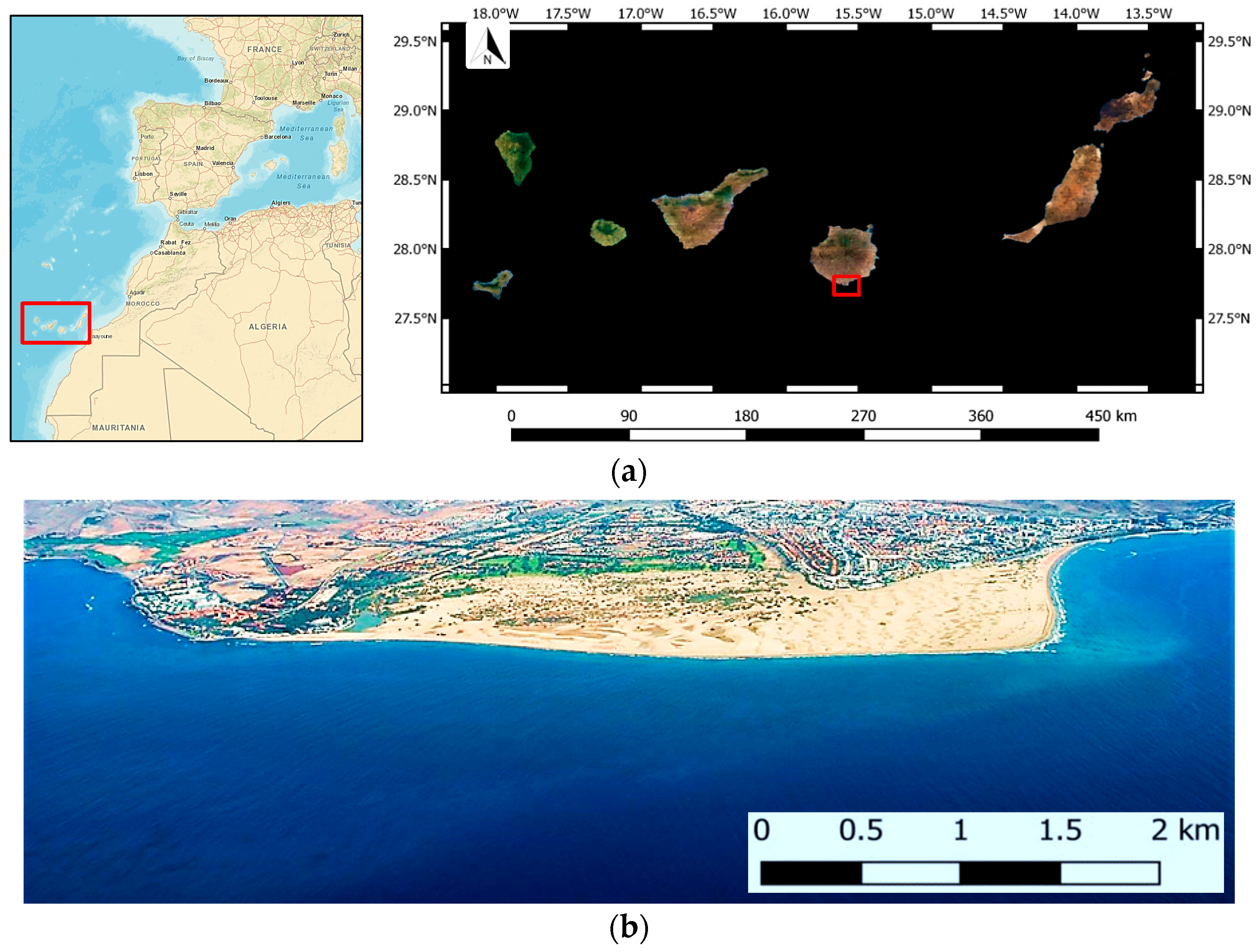
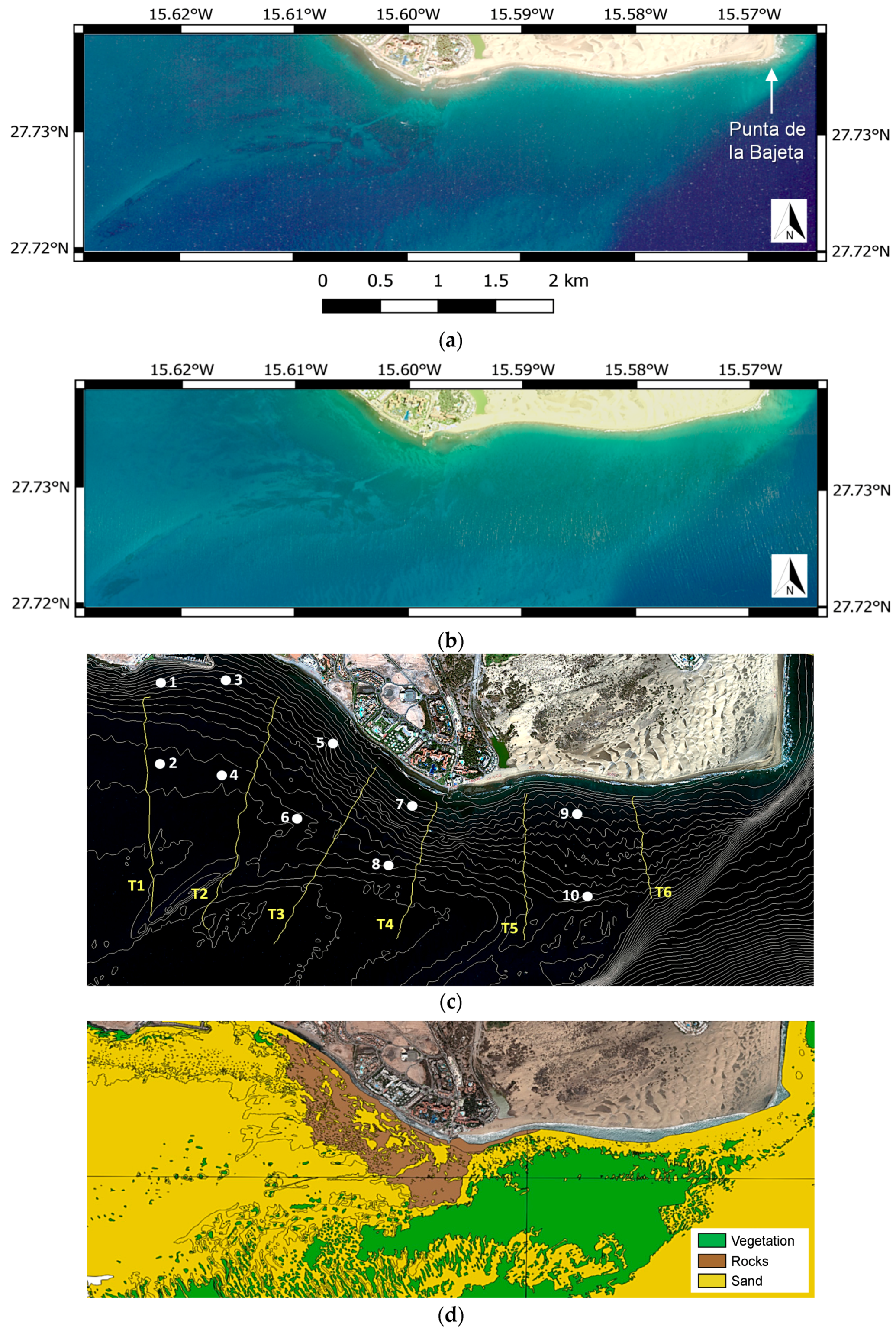
2.1. Study Area

The Maspalomas Natural Reserve (Gran Canaria, Spain) is an important coastal-dune ecosystem covering approximately 4 km² and with a high touristic pressure, visited by more than 2 million people each year. The marine vegetation in the coastal fringe is basically composed of seagrass beds. The most abundant seagrass species is Cymodocea nodosa but, more recently, the Caulerpa prolifera green algae has also become dominant in this area. Figure 1 shows the geographic location of Maspalomas.

2.2. Multisensor Remotely Sensed Data

A flight campaign was performed on June 2, 2017 and data were collected at 2.5 m resolution with the Airborne Hyperspectral Scanner (AHS). The AHS sensor (developed by ArgonST, USA) is operated by the Spanish Aerospace Institute (INTA) onboard the CASA 212-200 Paternina. AHS incorporates an 80-band imaging radiometer covering the range from 0.43 to 12.8 μm. In our study, only the first 20 channels were selected, covering the visible and near-infrared (NIR) spectrum from 0.434 to 1.015 μm with 12-bits of radiometric resolution [41]. Additionally, a WorldView-2 (WV-2) image collected on January 17, 2013 was considered for this study. Its sensor has a radiometric resolution of 11 bits and a spatial resolution, at the nadir, of 1.8 m for the 8 multispectral bands (0.40–1.04 μm). The panchromatic wideband was not used because this channel only provides information about the seabed in the very first meters of depth and, in consequence, pansharpening algorithms are not effective.

Table 1. Airborne Hyperspectral Scanner (AHS) and Worldview-2 spectral channels.

Sensor	Spectral Band	Wavelength (nm)	Bandwidth (nm)
AHS	Visible and Near-IR (20 channels)	434–1015	28–30
WV-2	Coastal Blue	400–450	47.3
	Blue	450–510	54.3
	Green	510–580	63.0
	Yellow	585–625	37.4
	Red	630–690	57.4
	Red-edge	705–745	39.3
	Near-IR 1	770–895	98.9
	Near-IR 2	860–1040	99.6
	Panchromatic	450–800	284.6

includes the spectral characteristics of both sensors and Figure 2a,b show the Worldview and AHS imagery for the area of interest processed in this work, respectively.

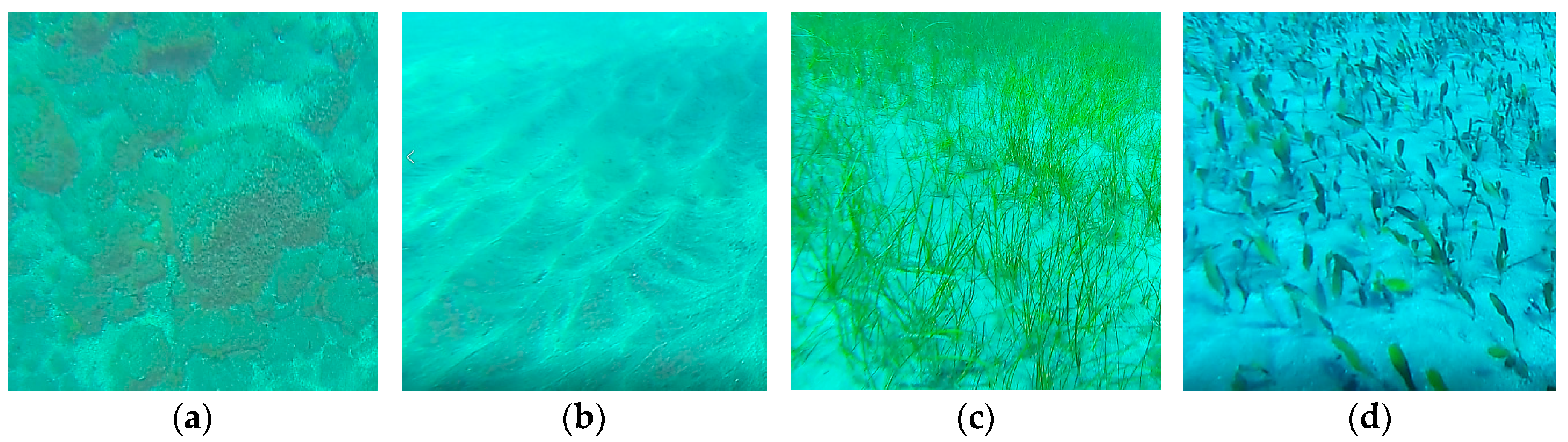
2.3. In-Situ Measurements

In-situ data were acquired simultaneously to the AHS campaign. A total of 6 transects were performed, measuring the bathymetry using an ecosounder Reson Navisound 110 and recording images of the seafloor using two different video cameras (Neptune and Go Pro Hero 3+). Precise geographic and temporal information was provided by a differential GPS receiver model Trimble DSM132. Ten additional sites visited during 2015 were also used in the analysis, providing bathymetry and video records from the Go Pro camera. The variation of the sea level due to tides and waves was obtained from a nearby calibrated tide gauge.

Figure 2c presents the real ship transects during the 2017 campaign, as well as the sites monitored in 2015 (marked by yellow dots). Isobaths are also included, and the sites and equidistant transects are perpendicular to the shore to get the maximum information of the area at different depths up to 20 m.

Finally, to assess the accuracy of the benthic maps derived from HS and MS imagery, apart from the accurate information from the in-situ transect and sampling sites, a reference map providing global information for the whole area was desirable. Unfortunately, very limited cartography is available and the map considered (Figure 2d) is the reference map available of the Maspalomas coast, which is part of a Spanish coastline eco-cartographical study from a series of maritime engineering and marine ecology studies structured in a GIS [42].

This information was used just as a coarse reference, but the quantitative validation only considered the precise information measured during the campaigns of 2015 and 2017.

The data used in this study correspond to different years (2013 to 2017). However, the seabed of Maspalomas is in a fairly stable area with the exception of Punta de la Bajeta (marked in Figure 2a), which is the zone with the greatest topographic and sedimentary variability due to storms from the southwest.

The seafloor images recorded during the field campaign (see Figure 3 for examples) show the complexity to discriminate habitat classes because they are usually mixed. Especially, submerged green aquatic vegetation meadows grow on sandy bottoms, and they have low density and mainly live between 5 and 25 m depth. In addition, rocks are partially covered by algae making automated classifications more challenging.

2.4. Mapping Methodology

The overall processing protocol to generate the seabed maps is presented in Figure 4. Different inputs to the classification algorithm were analyzed to select the best methodology. Following, there is a detailed description of the different steps involved.

2.4.1. Multisensor Imagery Corrections

• Multispectral Satellite Imagery

DigitalGlobe owns and operates a world-class constellation of high resolution, high accuracy Earth imaging satellites. The acquired WV-2 image is the level 2 ortho-ready product that has the geometric correction implemented and a horizontal accuracy specification of 5 meters or better [43].

In coastal areas, radiometric and atmospheric corrections have proven to be a crucial step in the processing of high-resolution satellite images due to the low signal-to-noise ratio at sensor level. A comparative evaluation of advanced atmospheric models (FLAASH, ATCOR, and 6S) in the coastal area of Maspalomas using high-resolution WorldView-2 data showed that the 6S algorithm achieved the highest accuracy when the corrected reflectance was compared to field spectroradiometer data (RMSE of 0.0271 and bias of −0.0217) [14]. Hence, we have applied the 6S correction model but adapted to the WorldView-2 spectral response and to the particular scene geometry and date of the image. 6S is a radiative transfer model that generates the constants $\left(x_a, x_b and x_c\right)$ to estimate the surface (BOA: Bottom Of Atmosphere) reflectance by [14,44,45]:

$${\rho }_{BOA}^{\prime }=\frac{\left(x_a{L}_{TOA}\right)-x_b}{1+\left(x_c\left(\left(x_a{L}_{TOA}\right)-x_b\right)\right)}$$

(1)

corrected to consider the adjacency effect by:

$${\rho }_{BOA}={\rho }_{BOA}^{\prime }+\frac{{\tau }_o{}_{dif}}{{\tau }_o{}_{dir}}\left[{\rho }_{BOA}^{\prime }-\overline{\rho }\right]$$

(2)

where $L_{TOA}$ is the radiance measured by the sensor (TOA: Top Of Atmosphere), ${\rho }_{BOA}^{\prime }$ is the initially corrected surface reflectivity by the 6S model, ${\rho }_{BOA}$ is the surface reflectivity taking into account the adjacency effect, ${\tau }_o{}_{dif}$ and ${\tau }_o{}_{dir}$ are the diffuse and direct transmittances and $\overline{\rho }$ is the average reflectivity contribution from the pixel background [44].

Moreover, specular reflection of solar radiation is a serious disturbance for water quality, bathymetry, and benthic mapping in shallow-water environments. We applied the method suggested by References [15,16] to remove sunglint. Therefore, regions of the image having sunglint were selected, preferably areas of deep water. For each visible channel, all the pixels from these regions were included in a linear regression between the NIR against each visible band. Therefore, the reflectance of each pixel in the visible band i (${\rho }_{BOA,i}$) can be deglinted $\left({\rho }_{BOA,i}^{DG}\right)$ using the following equation:

$${\rho }_{BOA,i}^{DG}= {\rho }_{BOA,i}- b_i\ast \left({\rho }_{BOA,NIR}-MI{N}_{NIR}\right)$$

(3)

where b_i is the slope of the regression line for band i, ${\rho }_{BOA,NIR}$is the reflectance of the NIR channel and MIN_NIR corresponds to the minimum reflectance value of the NIR image.

Improvements in the glint removal algorithm were performed [46] because, for WorldView-2, all the sensor bands are not recording the energy at the same precise time. In addition, the deglinting process, in the presence of considerable waves, alters the spectral content of the image. To overcome this inconvenience, a histogram matching was applied to statistically equalize each channel after and before deglinting. Finally, to remove the foam caused by the waves (whitecaps), pixels achieving reflectance values above a threshold were replaced by interpolation [46].

Water column correction is a very complex matter due to the variability of the bottom type, water depth, and water attenuation (scattering and absorption in the water column). Lyzenga proposed a simpler depth invariant index [17] but, in the last decades, different water models have been developed. In this work, a radiative transfer model for coastal waters was implemented [14]. The assumption is that the water leaving radiance is not only caused by the water column (IOPs: water Inherent Optical Properties), but it is also affected by the seafloor albedo and its corresponding bathymetry. In particular, the Lee et al. [47] exponential expression was used, that is an improved version of the formulation proposed by Reference [22]. The model can be expressed by:

$$r_{rs}^m\left(\lambda \right)\approx r_{rs,\infty }\left(\lambda \right)\left(1-e^{-\left[\frac{1}{{\mu }_s^{sw}}+\frac{D_u^c}{{\mu }_v^{sw}}\right]k_{d}z}\right)+\frac{{\rho }_{alb}\left(\lambda \right)}{\pi }{e}^{-\left[\frac{1}{{\mu }_s^{sw}}+\frac{D_u^b}{{\mu }_v^{sw}}\right]k_{d}z}$$

(4)

where $r_{rs}^m\left(\lambda \right)$ is the modeled reflectivity, $r_{rs,\infty }\left(\lambda \right)$ corresponds to the reflectivity below the sea surface for deep waters generated by the IOPs, ${\rho }_{alb}\left(\lambda \right)$ represents the seafloor reflectivity (albedo), z stands for the bathymetry, $k_d$ is the water diffuse attenuation coefficient, ${\mu }_s^{sw}$ and ${\mu }_v^{sw}$ allow the corrections in the sun and sensor trajectories for the downwards and upwards directions, and, finally, $D_u^c$ and $D_u^b$ are light diffusion ascending factors due to the water column and the bottom reflectivity, respectively.

As proposed in Reference [48], the Fully Constrained Linear Unmixing method (FCLU) was used to model the seabed albedo. The albedo is obtained as the sum of the products of the abundances of the $p$ pure benthic elements $\left(a{b}_i\right)$ by their albedo for each wavelength ($e{m}_i\left(\lambda \right)$):

$${\rho }_{alb}\left(\lambda \right)={\displaystyle \sum }_i^{P}a{b}_i\ast e{m}_i\left(\lambda \right)$$

(5)

Due to the limitations of the sensitivity of the multispectral sensors, we decided to use the three most significant and separable spectra of the seabed coverage in the area (sand, rocks and green vegetation). The radiative transfer modeling was adapted to multispectral sensors by integrating the result of the monochromatic model for the bandwidths of the 6 first channels of WV-2.

• Airborne Hyperspectral Imagery

Regarding the AHS geometric accuracy, the airborne inertial system achieves a final angular precision of 0.008° for the roll and the pitch, and 0.015° for the true heading; and a 12 channels GPS receiver provides trajectory location with accuracies of 5 to 10 cm [41].

For the hyperspectral data, atmospheric and illumination corrections were performed by INTA using the ATCOR4 model [41,49]. ATCOR4 is the ATCOR specific version for hyperspectral airborne data, and it is based on the MODTRAN-5 radiative transfer code.

The multispectral channels of the AHS sensor are somewhat narrower than the WV2 channels, providing, in the visible range, 12 multispectral channels instead of the 6 of the WV2. The greater number of channels implies greater spectral information and, therefore, an assumed greater sensitivity in the classification of the benthic classes. In any case, the methodology carried out for the elimination of the specular solar brightness, and the radiative transfer modeling is identical to that applied to WV-2.

Finally, land and deep water masks were applied to the corrected bands after both sensors have been homogenized in terms of resolution and have been spatially aligned using a large database of singular and well-distributed ground control points. Seafloor is difficult to properly monitor over 20 m depth in this area using satellite or airborne remote sensing imagery; therefore, a mask was applied at the 20 m isobath.

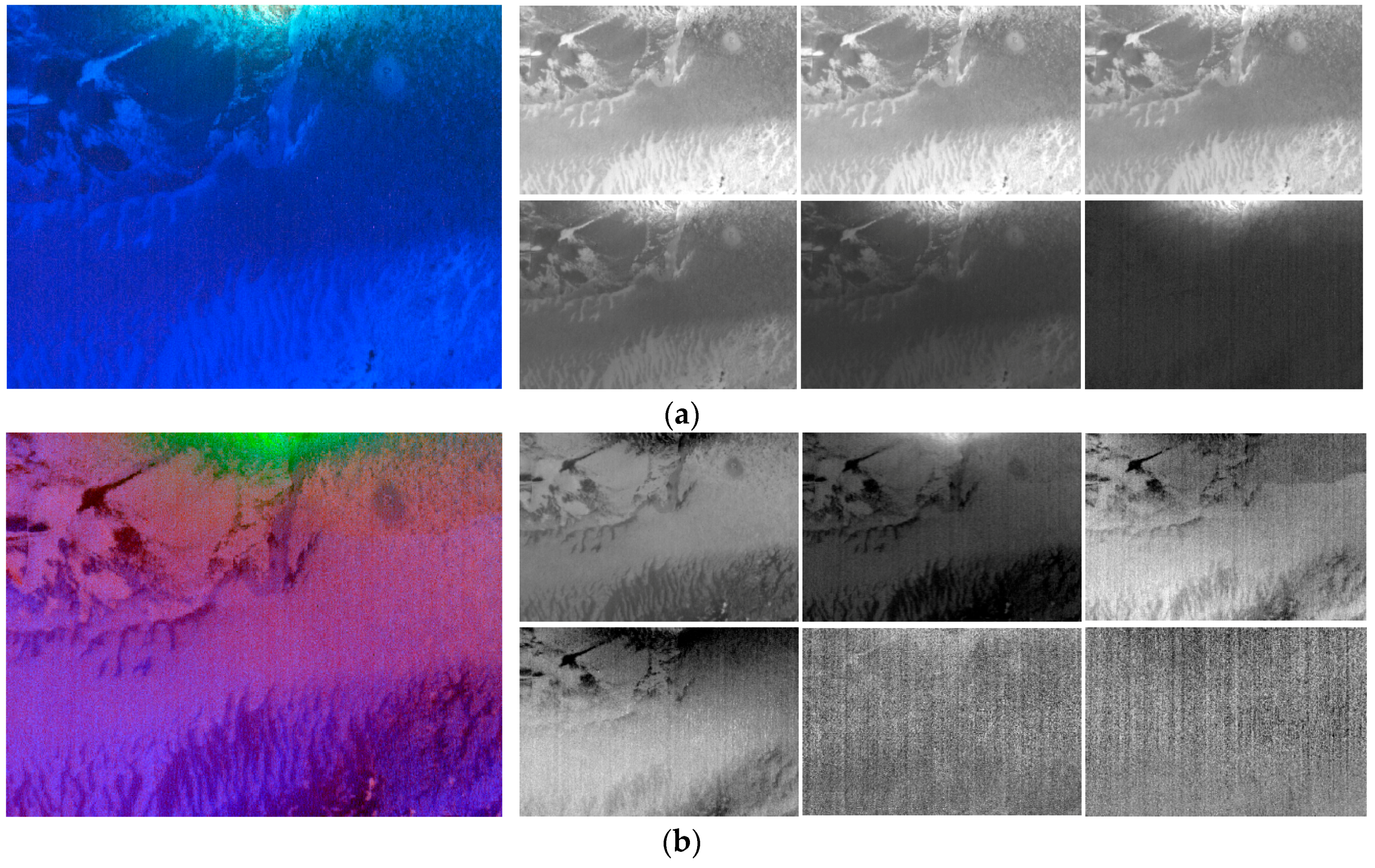
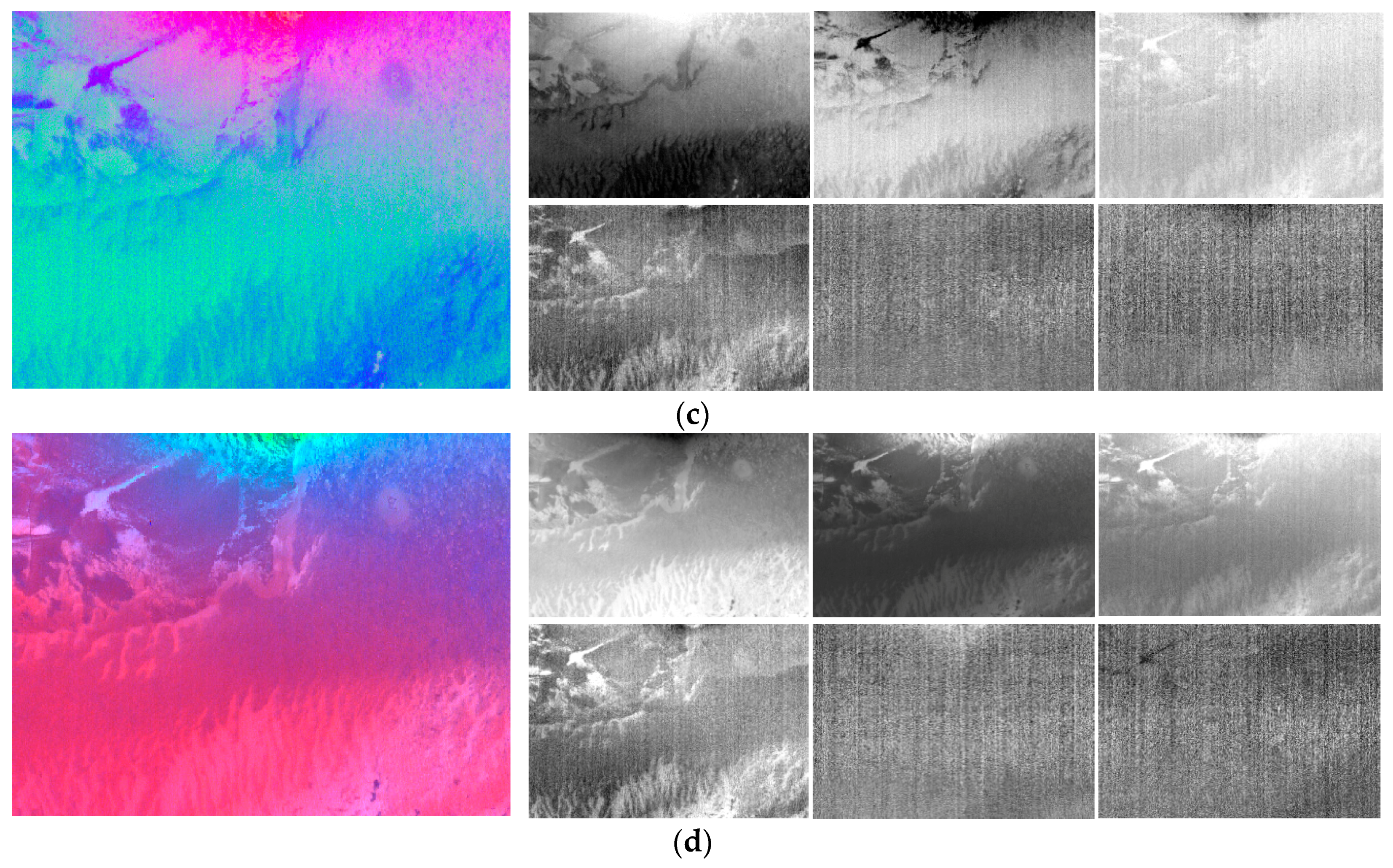
2.4.2. Feature Extraction

In addition to the spectral channels provided by each sensor, we also studied the inclusion of additional information to check the possible increase in classification performance. Therefore, we considered adding, to the multispectral or hyperspectral bands, components after Principal Component Analysis (PCA), Independent Component Analysis (ICA) and Minimum Noise Fraction (MNF) transforms; textural features to enrich the spatial information, and abundance maps extracted from linear unmixing techniques. Next, the feature extraction techniques are explained in more detail.

• Image Transforms

In hyperspectral imagery, the high number of narrow bands requires an increase in the number of training pixels to maintain a minimum statistical confidence and functionality for classification. This problem, known as the Hughes’ phenomenon [50] or the curse of dimensionality, can be addressed by overcoming data redundancy. Several transforms have been proposed in the last decades to extract reliable information, reducing redundancy and noise. Traditional feature-extraction techniques, mainly applied to reduce the dimensionality of hyperspectral data, are PCA, ICA, and MNF [51].

PCA uses an orthogonal transformation to convert a set of correlated bands into a new set of uncorrelated components [52]. PCA is frequently applied for dimensionality reduction because it retains most of the information of the original data in the first principal components. In consequence, computation times decrease, and the Hughes’ phenomenon is avoided, and, accordingly, the reduction of the considered components allows obtaining more precise thematic maps [53].

ICA decomposes the set of image bands into a linear combination of independent source signals [54]. ICA not only decorrelates second-order statistics, like PCA does but also decreases higher-order dependencies, generating a new set of components as independent as possible. It is an alternative approach to PCA for dimensionality reduction.

MNF Rotation is a linear transformation to segregate noise in the data and to reduce the computational requirements for subsequent processing [55]. This MNF transformation orders the new components so that they maximize the signal-to-noise ratio, rather than the information content [56]. MNF, apart from reducing the dimensionality, can be used to remove noise from data by performing a forward transform, by determining which bands contain the coherent information, by examining the images and eigenvalues, and then applying the inverse transform using only the appropriate bands, or adding as well the filtered or smoothed noisy bands.

• Texture Maps

We analyzed the inclusion of spatial information into the classification to improve the separability between the classes. There is a wide variety of texture measurements and, in this experiment, the parameters used were derived from the Gray-Level-Co-occurrence Matrix (GLCM) [57]. The main idea of the GLCM measurements is that the texture information contained in an image is based on the adjacency relationship between gray levels in the image. The relationship of the occurrence frequencies between pixel pairs can be calculated reliably for specific directions and distances between them.

After a preliminary analysis, we observed that most of the texture maps, derived from the co-occurrence matrix, were very similar (variance, entropy, dissimilarity, etc.). Therefore, to avoid the inclusion of redundant information, only the mean and variance parameters were finally used. Instead of applying the GLCM to each original band and, consequently, to have a large dataset of redundant texture information, the GLCM was only applied to the first component of the PCA and MNF transforms.

• Abundance Maps

In general, many pixels in the image represent a mixture of spectral signatures from different classes (e.g., seagrass and sand). In this context, mixing models estimate the contribution (abundance) of each endmember (pure class) to the total reflectance of each pixel. Linear mixing models provide adequate results in a large number of applications [27], and while non-linear models can be more precise, they require detailed information about the geometry and physical properties of the objects, which is not usually available and, thus, hinders its usefulness.

There are different strategies for the selection of pure pixels. In this work, as supervised classification techniques were applied, the training regions selected for each class were used to get the spectral signatures of each endmember.

After the application of unmixing techniques, an abundance map for each class to be discriminated was generated. Each map represents the percentage of contribution of a class to the total reflectance value of the pixel. In consequence, maps have values between 0 and 1 and, if a pixel is a mixture of different classes, the abundance of each class is obtained.

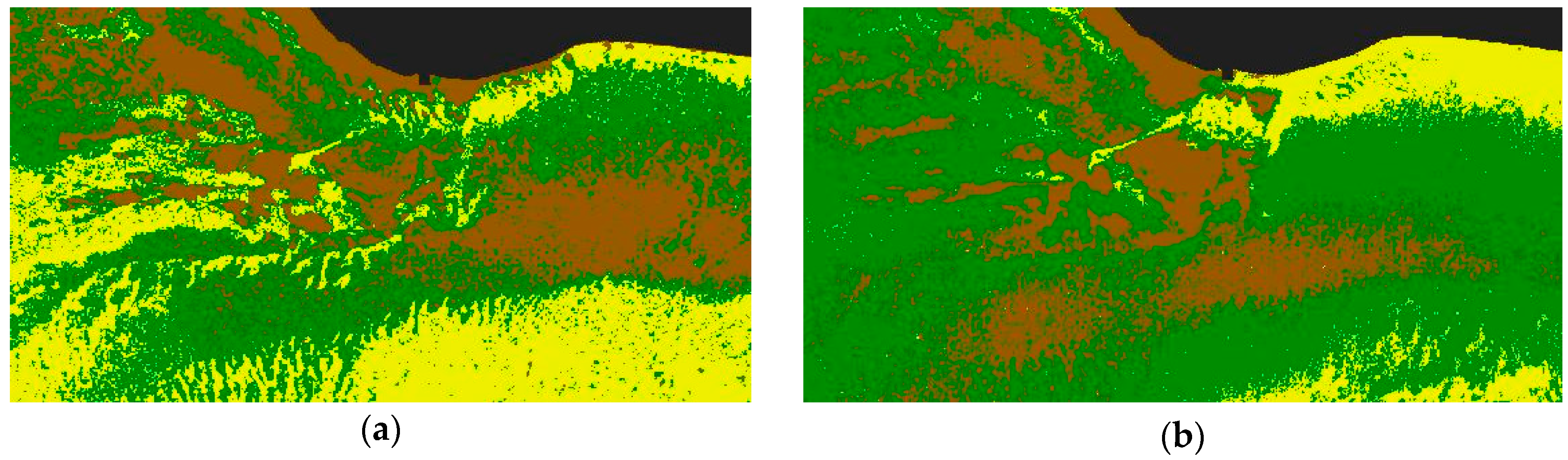
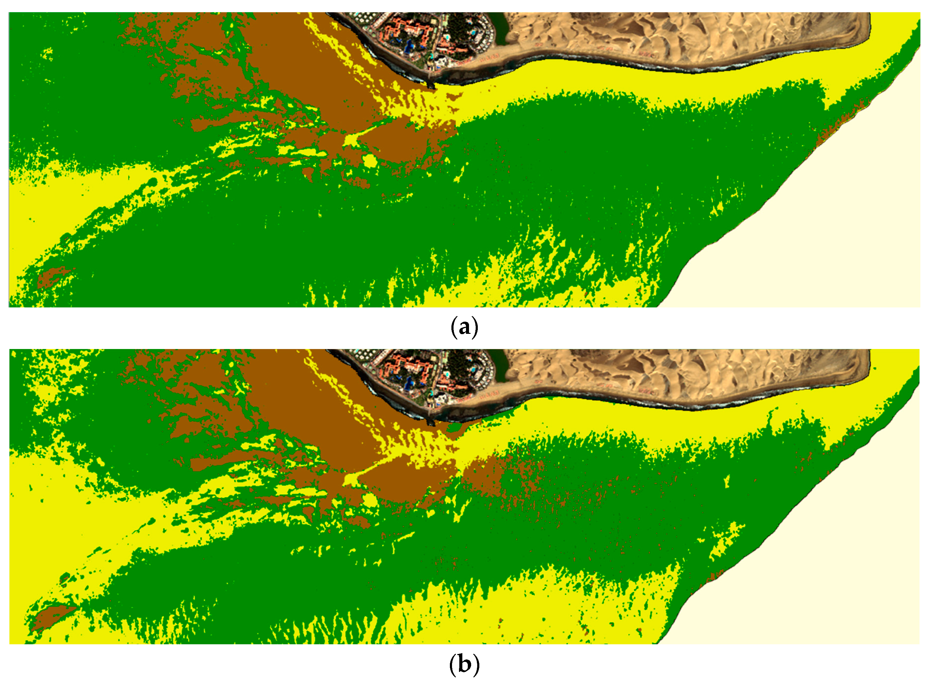
2.4.3. Classification

We used pixel and object-based supervised classifiers [51,58,59]. Specifically, Maximum Likelihood (ML), Spectral Angle Mapper (SAM), and Support Vector Machine (SVM) algorithms were assessed.

ML classification is one of the most common supervised techniques used with remotely sensed data [51]. ML considers that each class can be modeled as a normal distribution, allowing to describe that class by a Gaussian probability function, from its vector of means and covariance matrix. ML assigns the pixel to the class that maximizes the probability function.

The SAM classifier [52] compares the similarity between two spectra from their angular deviation, assuming that they form two vectors in an n-dimensional space (n being the number of bands). This algorithm measures the similarity as a function of the angle both vectors form in such a space.

SVM [60] is a machine learning algorithm to discriminate two classes by fitting an optimal hyperplane to separate the training samples of each class. The samples closest to the decision boundary are the so-called support vectors. SVM has been efficiently applied to classify both linear and nonlinearly separable classes applying a kernel function into a higher dimensional space, whose new data distribution allows better fitting of a linear hyperplane. Although deep learning approaches are becoming popular [61], they require large training datasets, and that is a great inconvenience in many operational applications. In addition, a recent assessment comparing advanced classification methods (SVMs, random forests, neural networks, deep convolutional neural networks, logistic regression-based techniques, and sparse representation-based classifiers) demonstrated that SVM is widely used because of its accuracy, stability, automation, and simplicity [26]. After a detailed review of SVM literature [18,62,63,64] and many tests conducted using the SVM algorithm with high-resolution imagery [65,66], the Gaussian radial basis function kernel $K\left(x_i, x_j\right)$was selected for the SVM classification and their parameters were properly adjusted:

$$K\left(x_i, x_j\right)=e^{\left(-\frac{\Vert x_i-x_j{}^2\Vert }{2{\sigma }^2}\right)}$$

(6)

For the segmentation and merging steps in the object based classification (OBIA), after testing different combinations, using diverse features and number of bands, AHS channels 1 to 3 and WV-2 channel 1 were used. During the segmentation process, the image is divided into homogeneous regions according to several parameters (band weights, scale, color, shape, texture, etc.) defined by the operator, with the objective of creating the suitable object borders. We tested a multiresolution segmentation approach [67] and an algorithm based on watershed segmentation and merging stages [68]. An over-segmented image was preferred, and as soon as a suitable segmentation was attained, the classifier was applied.

Finally, the classification accuracy for each possible combination of input data was estimated using independent test regions of interest (ROIs) located in the image and computing the kappa coefficient, the confusion matrix, and its derived measures.

3. Results and Discussion

After the correction of each dataset (see Figure 4), three supervised classifiers were applied to different combinations of input data. All the analysis was performed for HS and MS imagery (AHS and WV-2, respectively) at the complex area of Maspalomas.

As seafloor reflectivity is very weak, and following the steps of Figure 4, precise preprocessing algorithms were applied to correct limitations in the sensor calibration, solar illumination geometry, viewing effects, as well as the atmospheric, sunglint, and water column disturbances. In this sense, geometric, radiometric and atmospheric corrections were performed. As specified, 6S was selected to model the atmosphere and to remove the absorption and scattering effects in the multispectral image [14], and ATCOR4 for the hyperspectral data [49]. This selection took into account the results of a previous validation campaign comparing real sea surface reflectance recorded by a field spectroradiometer (ADS Fieldspec 3) and the reflectance estimated for WV-2 data using different models. Next, deglinting algorithms were applied to eliminate the solar glint and whitecaps over both datasets. Finally, the seafloor albedo was generated applying the radiative transfer model described in Section 2.4.1. As shown in Figure 5, for a small area, the improvement is considerable, especially for the AHS data, as some areas were severely affected by de-sunglint.

A preliminary analysis was performed to find the most suitable corrected imagery to address the classification problem. Specifically, images obtained after the different pre-processing steps were assessed to identify the more reliable data source for the mapping production. The following thematic classes were considered: sand (yellow), rocks (brown) and Cymodocea or Caulerpa (green). Using the information from the ship transects and sampling sites (Figure 2c), sets of training and validation regions were generated including regions of each class at five-meter step depths from 5 to 20 m. Approximately, 3000 and 6000 pixels per class were selected for the training and test ROIs, respectively. The class pair separability (Jeffries-Matusita distance [52]) in the bands ranges from 1.218 to 1.693 for WV-2 and between 1.802 and 1.985 for AHS. These values corroborate a better discrimination capability of HS data as more spectral richness is available.

Table 2. Overall accuracy (%) of Maximum Likelihood (ML), Support Vector Machine (SVM) and Spectral Angle Mapper (SAM) for Airborne Hyperspectral Scanner (AHS) and Worldview-2 (WV-2), and the different input combinations after each correction stage (AC: Atmospheric correction, SC: Sunglint Correction and WCC: Water Column Correction. Best accuracies marked in bold).

Sensor	Input	ML	SVM	SAM
AHS	AC	88.87	91.34	58.13
	AC+SC	91.81	92.01	58.35
	AC+SC+WCC	82.42	84.66	40.44
WV-2	AC	88.08	74.66	54.68
	AC+SC	88.66	80.63	58.37
	AC+SC+WCC	76.76	69.17	45.76

presents the results of applying the three supervised classifiers to the data after the atmospheric, sunglint, and water column corrections. The same independent training and validation regions of interest were used in all the experiments. As expected, the airborne hyperspectral imagery allows a better classification than the satellite multispectral data (92.01% with respect to 88.66%). It can be appreciated that the best overall accuracy was achieved after the deglinting step. The water column removal did not improve the seafloor mapping, even after applying a complex radiative model. Even providing adjusted water IOPs and bathymetry values, the modeling of the background albedo by linear mixing of benthic classes in this complex area does not seem adequate for the subsequent classification. The very low reflectivity of the coastal bottom, which usually contributes less than 1% of the radiation observed by the sensor, produces errors in the adjustment of the abundances of the modeled pure benthic elements. Clearly, the model considered has to be further improved. As indicated, the water column modelling in coastal areas is complex and depends on the water quality parameters, as well as the bathymetry and the type of seabed. For this reason, this preprocessing is not always considered and some studies demonstrate that better results are not always achieved [18,20,40]. Finally, regarding the classification algorithm, SVM is the most appropriate approach for AHS but Maximum Likelihood works better with WV-2.

Figure 6 shows examples of seafloor maps generated for the AHS sensor, with SVM, and for the WV-2 data using the ML classifier. Comparing the results with the reference benthic map (Figure 2d) and the available video records from the ship transects, higher accuracy can be noted for AHS and using the imagery after the atmospheric and sunglint correction (middle row). Excessive amount of submerged vegetation is identified for WV-2 and some rocks incorrectly appear on the right side when these pixels should be labeled as vegetation.

To improve the previous seabed cartography, a detailed feature extraction and classification assessment was only performed using the preprocessed data after the atmospheric and sunglint correction stages.

As stated in Section 2.4.2, to improve the benthic maps, additional information was obtained using feature extraction techniques. In particular, PCA, ICA and MNF were applied to the corrected spectral bands. In the analysis, the classifier performance was assessed including the complete new set of components after these transforms and, in addition, the best components were also tested discarding noisy bands. Figure 7 shows the first bands of each transform, as well as the original spectral bands as a reference (the remaining bands were not displayed as they are too noisy). Regarding the spectral channels, we can appreciate that only shorter wavelengths (first bands) can reach the seafloor and, in consequence, even dealing with hyperspectral data only a few channels are really valuable to map benthic habitats up to a depth of 20 m. On the other hand, PCA, ICA and MNF provide useful information in the first four components. The true color image and false color composites using the first three components are also included, and it is possible to check the worse behavior of ICA and the noise removal effect of MNF.

Additional textural parameters and abundance maps after unmixing were also inputted to the classifiers as auxiliary information.

Table 3. Overall accuracy (%) of ML, SVM, and SAM for AHS and WV, and the different input combinations (Best accuracies marked in bold).

Sensor	Input	ML	SVM	SAM	Average
AHS	Bands (21)	91.81	92.01	58.35	80.72
	Bands 1-8 (8)	93.77	84.56	57.36	78.56
	PCA (21)	91.81	94.48	47.39	77.89
	PCA 1-4 (4)	93.25	92.39	50.54	78.73
	ICA (21)	91.81	85.57	29.58	68.99
	ICA 1-4 (4)	88.61	79.29	40.92	69.61
	MNF (21)	91.81	90.60	36.59	73.00
	MNF 1-4 (4)	93.57	90.11	39.08	74.25
	LU_ab (3)	90.63	73.33	48.57	70.84
	B+LU_ab (24)	92.20	90.04	58.35	80.20
	B+Text_PCA1 (23)	91.30	97.29	58.35	82.31
	B+Text_MNF1 (23)	92.30	85.90	58.35	78.85
	OBIA Bands (21)	85.70	97.36	61.51	81.52
	Average	91.43	88.69	49.61	76.58
WV-2	Bands (8)	88.66	80.63	58.37	75.89
	Bands 1-3 (3)	85.48	79.97	52.86	72.77
	PCA (8)	88.66	80.91	69.13	79.57
	PCA 1-4 (4)	87.60	82.27	68.79	79.55
	ICA (8)	88.66	70.90	58.26	72.61
	ICA 2-5 (4)	76.44	71.72	34.40	60.85
	MNF (8)	88.66	80.91	53.44	74.34
	MNF 1-4 (4)	88.34	80.52	53.31	74.06
	LU_ab(3)	87.70	70.16	74.39	77.42
	B+LU_ab (11)	88.71	81.16	74.38	81.42
	B+Text_PCA1 (10)	87.50	81.44	58.75	75.90
	B+Text_MNF1 (10)	88.41	78.45	57.57	74.81
	OBIA Bands (8)	82.27	91.66	64.55	79.49
	Average	86.70	79.28	59.86	75.28

summarizes the AHS and WV-2 accuracy results of each classifier for the following input combinations:

• Spectral bands after atmospheric and sunglint corrections.
• Components after the application of three-dimensionality reduction techniques (PCA, ICA, and MNF). The complete dataset and a reduced number of bands or components were both tested.
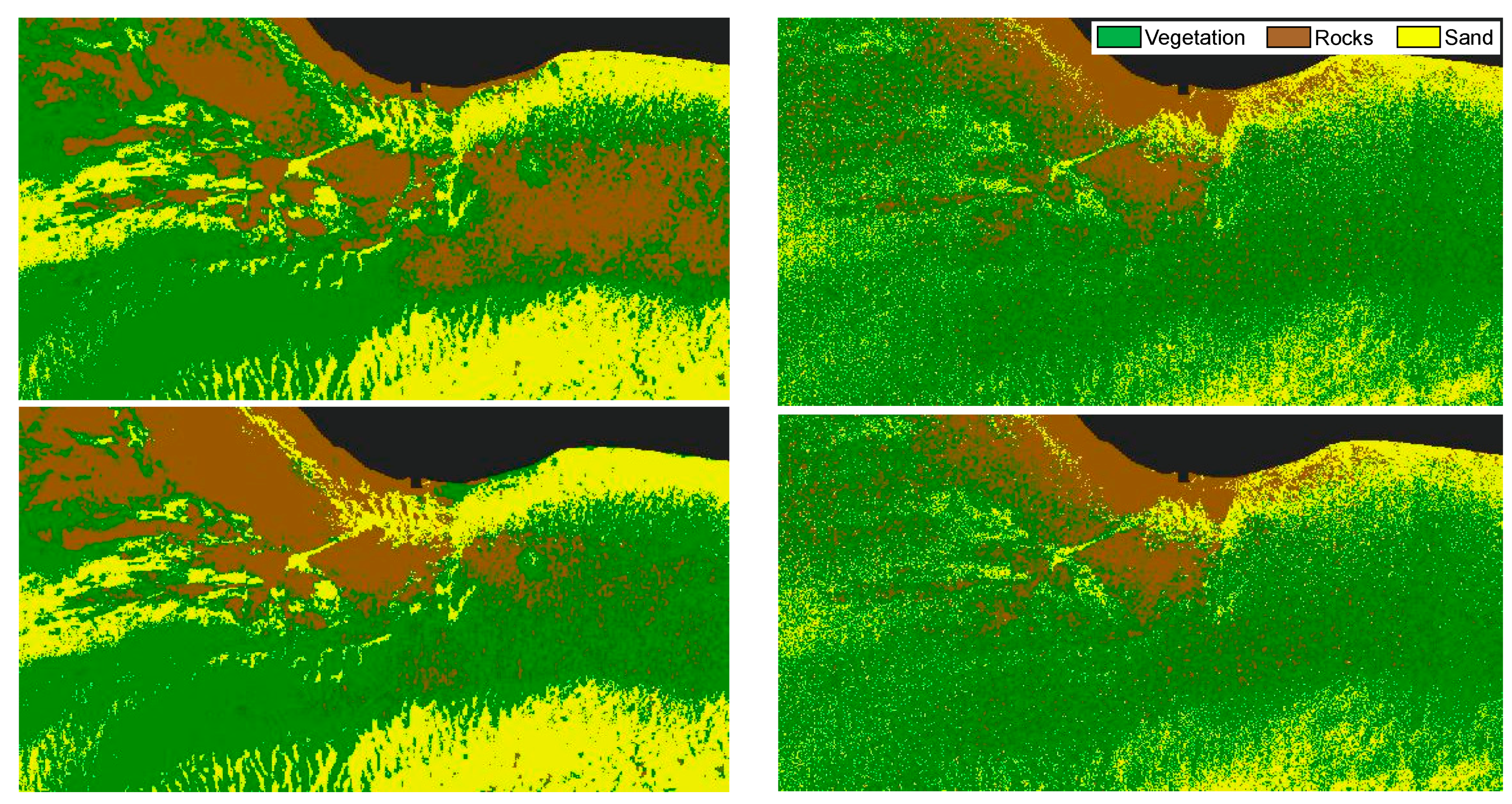
• Abundance maps of each class after the application of linear unmixing techniques.
• Texture information (mean and variance) extracted from the first PCA/MNF component.

Pixel-based classification was applied to the previous options and, finally, object-based classification was applied to the spectral bands.

With respect to the sensors, we can appreciate that AHS provides better accuracy than WV-2, as expected, mainly due to the availability of additional bands and a better radiometric resolution. Specifically, a major improvement is attained for SVM (mean accuracy increase of 9.5%) than for ML (4.7% average increase).

Concerning the classification algorithms, SAM did not work properly because, even being more insensitive to variations of the bathymetry, classes are spectrally overlapped, and only very few bands are useful due to the water column attenuation. SVM is the algorithm achieving the best accuracy, but the simpler and faster ML demonstrates good performance and, in many cases, better than SVM (average results in Table 3 confirm it). Actually, Figure 8 presents the comparative performance of both classifiers, and it can be appreciated that ML is more robust, providing more stable results regardless of the input information used or the number of bands considered. Specifically, the standard deviation (averaged for AHS and WV-2) of the overall accuracy for the different combinations is 2.9% for ML and 6.4% for SVM.

PCA and MNF perform much better than ICA, but the improvement is, in general, negligible with respect to the original bands. Also, the reduction of the number of bands/components to avoid the Hughes’ phenomenon is basically not increasing the classification accuracy except for ML and the hyperspectral data. The number of training pixels for each class is high enough (3000), and that could be a possible explanation.

The application of unmixing techniques before the classification did not improve the accuracy due to the small number of bands actually available. It can be appreciated the degraded performance of SVM when only the three abundances are considered in the classification scheme.

Finally, texture information is a feature that can be included in the final methodology as precision values in some circumstances increase the performance. Specifically, the improvement is more evident for SVM and using the texture information provided by the first component of PCA. For ML, texture generally does not provide a better accuracy of the benthic map.

It is important to highlight that results obtained by the object-based classification techniques (OBIA) are not always the best. Basically, OBIA only provides superior performance than pixel-based techniques for the SVM algorithm. However, results are quite dependent on the type of segmentation considered.

In general, the overall accuracies for ML and SVM are high as few classes are considered and the validation pixels chosen to numerically assess accuracy were selected in clear and central locations of each seabed type. In any case, the relative results between the different classifiers and input combinations displayed in Table 3 are reliable.

Figure 9 includes an example of the AHS and WV-2 segmentation for a specific area. AHS provides more detailed information and, in consequence, the number of objects increases.

Figure 10 compares the best pixel-based seafloor maps generated by ML and SVM for the AHS image. A majority filter of 5 × 5 window size was applied to remove the salt and pepper effect. Both maps are very accurate, but ML overestimates vegetation (green) in some specific areas, while SVM the rocks (brown) in others. Finally, Figure 11 shows the best maps for each sensor obtained using the object-based classification with the SVM algorithm. Results are similar and, in general, match the available eco-cartographic map included in Figure 2d, except for the western side of the area. In any case, as indicated, this map was just considered a coarse reference and really ship transects T1 and T2 in Figure 2c demonstrate the existence of vegetation meadows in that area, in agreement with AHS and WV-2 maps. It is also important to highlight that a vulnerable and complex ecosystem was studied where the density of submerged green aquatic vegetation beds is quite low and, therefore, there is a considerable mixture of sand and plant contributions in each pixel of the image.

These methodologies will be shortly applied to generate precise benthic maps of natural protected ecosystems in other vulnerable coastal ecosystems. In addition, these will be applied to hyperspectral imagery recorded from drone platforms with the goal of discriminating between the different vegetation species.

4. Conclusions

A comprehensive analysis was performed to identify the best input dataset and to obtain a robust classification methodology to generate accurate benthic habitat maps. The assessment considered pixel-based and object-oriented classification methods in shallow waters using hyperspectral and multispectral data.

A vulnerable and complex coastal ecosystem was selected where the submerged green aquatic vegetation meadows to be classified are located at depths between 5 and 20 meters and have low density, implying the availability of very few spectral channels with information and a considerable mixing of spectral contributions in each image pixel.

Appropriate and improved atmospheric and sunglint correction techniques were applied to the HS and MS data. Next, a water radiative transfer model was also considered to remove the water column disturbances and to generate the seafloor albedo maps. A preliminary analysis was performed to identify the most suitable preprocessed imagery to be used for seabed classification. Three different supervised classifiers (maximum likelihood, support vector machines, and spectral angle mapper) were tested.

A detailed analysis of different feature extraction methods was performed with the goal to increase the discrimination capability of the classifiers. To our knowledge, the effect of three rotation transforms to generate benthic maps was assessed for the first time. Texture parameters were, as well, added to check whether spatial and context information improve classifications. Finally, the inclusion of abundance maps for each cover, obtained by the application of linear unmixing algorithms, was also considered but, given the small number of spectral bands actually reaching the seafloor, results were not fully satisfactory. The best results were produced by SVM and the OBIA approach. However, to generate benthic habitat maps, the simple ML has shown an excellent performance and superior stability and robustness than SVM (average overall accuracies over 3% and 7% for AHS and WV-2 data, respectively).

In summary, a robust methodology was identified, including the best correction techniques, feature extraction methods, and classification approaches, and it was successfully applied to multispectral and hyperspectral data in a complex coastal zone.

References

1. Horning, E.; Robinson, J.; Sterling, E.; Turner, W.; Spector, S. Remote Sensing for Ecology and Conservation; Oxford University Press: New York, NY, USA, 2010; ISBN 978-0-19-921995-7. [Google Scholar]
2. Wang, Y. Remote Sensing of Coastal Environments; Taylor and Francis Series; CRC Press: Boca Raton, FL, USA, 2010; ISBN 978-1-42-009442-8. [Google Scholar]
3. Hossain, M.S.; Bujang, J.S.; Zakaria, M.H.; Hashim, M. The application of remote sensing to seagrass ecosystems: An overview and future research prospects. Int. J. Remote Sens. 2015, 36, 61–114. [Google Scholar] [CrossRef]
4. Lyons, M.; Phinn, S.; Roelfsema, C. Integrating Quickbird multi-spectral satellite and field data: Mapping bathymetry, seagrass cover, seagrass species and change in Moreton bay, Australia in 2004 and 2007. Remote Sens. 2011, 3, 42–64. [Google Scholar] [CrossRef]
5. Knudby, A.; Nordlund, L. Remote Sensing of Seagrasses in a Patchy Multi-Species Environment. Int. J. Remote Sens. 2011, 32, 2227–2244. [Google Scholar] [CrossRef]
6. Eugenio, F.; Marcello, J.; Martin, J. High-resolution maps of bathymetry and benthic habitats in shallow-water environments using multispectral remote sensing imagery. IEEE Trans. Geosci. Remote Sens. 2015, 53, 3539–3549. [Google Scholar] [CrossRef]
7. Rani, N.; Mandla, V.R.; Singh, T. Evaluation of atmospheric corrections on hyperspectral data with special reference to mineral mapping. Geosci. Front. 2017, 8, 797–808. [Google Scholar] [CrossRef]
8. Chavez, P.S. An improved dark-object subtraction technique for atmospheric scattering correction of multispectral data. Remote Sens. Environ. 1988, 24, 459–479. [Google Scholar] [CrossRef]
9. Chavez, P.S. Image-Based Atmospheric Corrections. Revisited and Improved. Photogramm. Eng. Remote Sens. 1996, 62, 1025–1036. [Google Scholar]
10. Bernstein, L.S.; Adler-Golden, S.M.; Jin, X.; Gregor, B.; Sundberg, R.L. Quick atmospheric correction (QUAC) code for VNIR-SWIR spectral imagery: Algorithm details. In Proceedings of the IEEE Workshop on Hyperspectral Image and Signal Processing: Evolution in Remote Sensing (WHISPERS), Shanghai, China, 4–7 June 2012. [Google Scholar]
11. Marcello, J.; Eugenio, F.; Perdomo, U.; Medina, A. Assessment of atmospheric algorithms to retrieve vegetation in natural protected areas using multispectral high resolution imagery. Sensors 2016, 16, 1624. [Google Scholar] [CrossRef] [PubMed]
12. Adler-Golden, S.M.; Matthew, M.W.; Bernstein, L.S.; Levine, R.Y.; Berk, A.; Richtsmeier, S.C.; Acharya, P.K.; Anderson, G.P.; Felde, G.; Gardner, J.; et al. Atmospheric Correction for Short-Wave Spectral Imagery based on MODTRAN4. In Imaging Spectrometry V; International Society for Optics and Photonics: Bellingham, WA, USA, 1999; Volume 3753. [Google Scholar]
13. Gao, B.-C.; Davis Curtiss, O.; Goetz, A.F.H. A review of atmospheric correction techniques for hyperspectral remote sensing of land surfaces and ocean colour. In Proceedings of the IEEE International Geoscience and Remote Sensing Symposium, Denver, CO, USA, 31 July–4 August 2006. [Google Scholar] [CrossRef]
14. Eugenio, F.; Marcello, J.; Martin, J.; Rodríguez-Esparragón, D. Benthic Habitat Mapping Using Multispectral High-Resolution Imagery: Evaluation of Shallow Water Atmospheric Correction Techniques. Sensors 2017, 17, 2639. [Google Scholar] [CrossRef] [PubMed]
15. Kay, S.; Hedley, J.; Lavender, S. Sun Glint Correction of High and Low Spatial Resolution Images of Aquatic Scenes: A Review of Methods for Visible and Near-Infrared Wavelengths. Remote Sens. 2009, 1, 697–730. [Google Scholar] [CrossRef]
16. Hedley, J.D.; Harborne, A.R.; Mumby, P.J. Simple and robust removal of sun glint for mapping shallow-water bentos. Int. J. Remote Sens. 2005, 26, 2107–2112. [Google Scholar] [CrossRef]
17. Lyzenga, D.R. Remote sensing of bottom reflectance and water attenuation parameters in shallow water using Aircraft and Landsat data. Int. J. Remote Sens. 1981, 2, 72–82. [Google Scholar] [CrossRef]
18. Traganos, D.; Reinartz, P. Mapping Mediterranean seagrasses with Sentinel-2 imagery. Mar. Pollut. Bull. 2017. [Google Scholar] [CrossRef] [PubMed]
19. Manessa, M.D.M.; Haidar, M.; Budhiman, S.; Winarso, G.; Kanno, A.; Sagawa, T.; Sekine, M. Evaluating the performance of Lyzenga’s water column correction in case-1 coral reef water using a simulated Wolrdview-2 imagery. In Proceedings of IOP Conference Series: Earth and Environmental Science; IOP Publishing: Bristol; IOP Publishing: Bristol, UK, 2016; Volume 47. [Google Scholar] [CrossRef]
20. Wicaksono, P. Improving the accuracy of Multispectral-based benthic habitats mapping using image rotations: The application of Principle Component Analysis and Independent Component Analysis. Eur. J. Remote Sens. 2016, 49, 433–463. [Google Scholar] [CrossRef]
21. Tamondong, A.M.; Blanco, A.C.; Fortes, M.D.; Nadaoka, K. Mapping of Seagrass and Other Bentic Habitat in Balinao, Pangasinan Using WorldView-2 Satellite Image. In Proceedings of the IEEE International Geoscience and Remote Sensing Symposium, Melbourne, Australia, 21–26 July 2013; pp. 1579–1582. [Google Scholar] [CrossRef]
22. Maritorena, S.; Morel, A.; Gentili, B. Diffuse reflectance of oceanic shallow waters: Influence of water depth and bottom albedo. Limnol. Oceanogr. 1994, 39, 1689–1703. [Google Scholar] [CrossRef] [Green Version]
23. Garcia, R.; Lee, A.; Hochberg, E.J. Hyperspectral Shallow-Water Remote Sensing with an Enhanced Benthic Classifier. Remote Sens. 2018, 10, 147. [Google Scholar] [CrossRef]
24. Loisel, H.; Stramski, D.; Dessailly, D.; Jamet, C.; Li, L.; Reynolds, R.A. An Inverse Model for Estimating the Optical Absorption and Backscattering Coefficients of Seawater From Remote-Sensing Reflectance Over a Broad Range of Oceanic and Coastal Marine Environments. J. Geophys. Res. Oceans 2018, 123, 2141–2171. [Google Scholar] [CrossRef]
25. Barnes, B.B.; Garcia, R.; Hu, C.; Lee, Z. Multi-band spectral matching inversion algorithm to derive water column properties in optically shallow waters: An optimization of parameterization. Remote Sens. Environ. 2018, 204, 424–438. [Google Scholar] [CrossRef]
26. Ghamisi, P.; Plaza, J.; Chen, Y.; Li, J.; Plaza, A. Advanced spectral classifiers for hyperspectral images. IEEE Geosci. Remote Sens. Mag. 2017, 5, 8–32. [Google Scholar] [CrossRef]
27. Bioucas, J.; Plaza, A.; Dobigeon, N.; Parente, M.; Du, Q.; Gader, P.; Chanussot, J. Hyperspectral unmixing overview: Geometrical, statistical, and sparse regression-based approaches. IEEE J. Sel. Top. Appl. Earth Obs. Remote Sens. 2012, 5, 354–379. [Google Scholar] [CrossRef]
28. Hedley, J.D.; Roelfsema, C.M.; Chollett, I.; Harborne, A.R.; Heron, S.F.; Weeks, S.; Skirving, W.J.; Strong, A.E.; Eakin, C.M.; Christensen, T.R.L.; et al. Remote Sensing of Coral Reefs for Monitoring and Management: A Review. Remote Sens. 2016, 8, 118. [Google Scholar] [CrossRef]
29. Roelfsema, C.; Kovacs, E.; Ortiz, J.C.; Wolff, N.H.; Callaghan, D.; Wettle, M.; Ronan, M.; Hamylton, S.M.; Mumby, P.J.; Phinn, S. Coral reef habitat mapping: A combination of object-based image analysis and ecological modelling. Remote Sens. Environ. 2018, 208, 27–41. [Google Scholar] [CrossRef]
30. Mohamed, H.; Nadaoka, K.; Nakamura, T. Assessment of Machine Learning Algorithms for Automatic Benthic Cover Monitoring and Mapping Using Towed Underwater Video Camera and High-Resolution Satellite Images. Remote Sens. 2018, 10, 773. [Google Scholar] [CrossRef]
31. Purkis, S.J. Remote Sensing Tropical Coral Reefs: The View from Above. Annu. Rev. Mar. Sci. 2018, 10, 149–168. [Google Scholar] [CrossRef] [PubMed]
32. Petit, T.; Bajjouk, T.; Mouquet, P.; Rochette, S.; Vozel, B.; Delacourt, C. Hyperspectral remote sensing of coral reefs by semi-analytical model inversion—Comparison of different inversion setups. Remote Sens. Environ. 2017, 190, 348–365. [Google Scholar] [CrossRef]
33. Zhang, C. Applying data fusion techniques for benthic habitat mapping and monitoring in a coral reef ecosystem. ISPRS J. Photogramm. Remote Sens. 2015, 104, 213–223. [Google Scholar] [CrossRef]
34. Leiper, I.A.; Phinn, S.R.; Roelfsema, C.M.; Joyce, K.E.; Dekker, A.G. Mapping Coral Reef Benthos, Substrates, and Bathymetry, Using Compact Airborne Spectrographic Imager (CASI) Data. Remote Sens. 2014, 6, 6423–6445. [Google Scholar] [CrossRef] [Green Version]
35. Roelfsema, C.; Kovacs, E.M.; Saunders, M.I.; Phinn, S.; Lyons, M.; Maxwell, P. Challenges of remote sensing for quantifying changes in large complex seagrass environments. Estuar. Coast. Shelf Sci. 2013, 133, 161–171. [Google Scholar] [CrossRef]
36. Baumstark, R.; Duffey, R.; Pu, R. Mapping seagrass and colonized hard bottom in Springs Coast, Florida using WorldView-2 satellite imagery. Estuar. Coast. Shelf Sci. 2016, 181, 83–92. [Google Scholar] [CrossRef]
37. Koedsin, W.; Intararuang, W.; Ritchie, R.J.; Huete, A. An Integrated Field and Remote Sensing Method for Mapping Seagrass Species, Cover, and Biomass in Southern Thailand. Remote Sens. 2016, 8, 292. [Google Scholar] [CrossRef]
38. Uhrin, A.V.; Townsend, P.A. Improved seagrass mapping using linear spectral unmixing of aerial photographs. Estuar. Coast. Shelf Sci. 2016, 171, 11–22. [Google Scholar] [CrossRef]
39. Valle, M.; Palà, V.; Lafon, V.; Dehouck, A.; Garmendia, J.M.; Borja, A.; Chust, G. Mapping estuarine habitats using airborne hyperspectral imagery, with special focus on seagrass meadows. Estuar. Coast. Shelf Sci. 2015, 164, 433–442. [Google Scholar] [CrossRef]
40. Zhang, C.; Selch, D.; Xie, Z.; Roberts, C.; Cooper, H.; Chen, G. Object-based benthic habitat mapping in the Florida Keys from hyperspectral imagery. Estuar. Coast. Shelf Sci. 2013, 134, 88–97. [Google Scholar] [CrossRef]
41. De Miguel, E.; Fernández-Renau, A.; Prado, E.; Jiménez, M.; Gutiérrez, O.; Linés, C.; Gómez, J.; Martín, A.I.; Muñoz, F. A review of INTA AHS PAF. EARSeL eProc. 2014, 13, 20–29. [Google Scholar]
42. Gesplan. Plan Regional de Ordenación de la Acuicultura de Canarias. Tomo I: Memoria de Información del Medio Natural Terrestre y Marino. Plano de Sustratos de Gran Canaria; Gobierno de Canarias: Las Palmas de Gran Canaria, Spain, 2013; pp. 1–344. [Google Scholar]
43. Digitalglobe. Accuracy of Worldview Products. White Paper. 2016. Available online: https://dg-cms-uploads-production.s3.amazonaws.com/uploads/document/file/38/DG_ACCURACY_WP_V3.pdf (accessed on 1 June 2018).
44. Vermote, E.; Tanré, D.; Deuzé, J.L.; Herman, M.; Morcrette, J.J.; Kotchenova, S.Y. Second Simulation of a Satellite Signal in the Solar Spectrum—Vector (6SV); 6S User Guide Version 3; NASA Goddard Space Flight Center: Greenbelt, MD, USA, 2006.
45. Kotchenova, S.Y.; Vermote, E.F.; Matarrese, R.; Klemm, F.J. Validation of vector version of 6s radiative transfer code for atmospheric correction of satellite data. Parth radiance. Appl. Opt. 2006, 45, 6762–6774. [Google Scholar] [CrossRef] [PubMed]
46. Martin, J.; Eugenio, F.; Marcello, J.; Medina, A. Automatic sunglint removal of multispectral WV-2 imagery for retrieving coastal shallow water parameters. Remote Sens. 2016, 8, 37. [Google Scholar] [CrossRef]
47. Lee, Z.; Carder, K.L.; Mobley, C.D.; Steward, R.G.; Patch, J.S. Hyperspectral remote sensing for shallow waters: 2. Deriving bottom depths and water properties by optimization. Appl. Opt. 1999, 38, 3831–3843. [Google Scholar] [CrossRef] [PubMed]
48. Heylen, R.; Burazerović, D.; Scheunders, P. Fully constrained least squares spectral unmixing by simplex projection. IEEE Trans. Geosci. Remote Sens. 2011, 49, 4112–4122. [Google Scholar] [CrossRef]
49. Richter, R.; Schläpfer, D. Geo-atmospheric processing of airborne imaging spectrometry data. Part 2: Atmospheric/Topographic correction. Int. J. Remote Sens. 2002, 23, 2631–2649. [Google Scholar] [CrossRef]
50. Hughes, G. On the mean accuracy of statistical pattern recognizers. IEEE Trans. Inf. Theory 1968, 14, 55–63. [Google Scholar] [CrossRef]
51. Ibarrola-Ulzurrun, E.; Marcello, J.; Gonzalo-Martin, C. Assessment of Component Selection Strategies in Hyperspectral Imagery. Entropy 2017, 19, 666. [Google Scholar] [CrossRef]
52. Richards, J.A. Remote Sensing Digital Image Analysis, 5th ed.; Springer: Berlin, Germany, 2013; ISBN 978-3-54-029711-6. [Google Scholar]
53. Benediktsson, J.A.; Ghamisi, P. Spectral-Spatial Classification of Hyperspectral Remote Sensing Images; Artech House: Boston, MA, USA, 2015; ISBN 978-1-60-807812-7. [Google Scholar]
54. Li, C.; Yin, J.; Zhao, J. Using improved ICA method for hyperspectral data classification. Arab. J. Sci. Eng. 2014, 39, 181–189. [Google Scholar] [CrossRef]
55. Green, A.A.; Berman, M.; Switzer, P.; Craig, M.D. A transformation for ordering multispectral data in terms of image quality with implications for noise removal. IEEE Trans. Geosci. Remote Sens. 1988, 26, 65–74. [Google Scholar] [CrossRef] [Green Version]
56. Luo, G.; Chen, G.; Tian, L.; Qin, K.; Qian, S.E. Minimum noise fraction versus principal component analysis as a preprocessing step for hyperspectral imagery denoising. Can. J. Remote Sens. 2016, 42, 106–116. [Google Scholar] [CrossRef]
57. Haralick, R.; Shanmugam, K.; Dinstein, I. Textural features for image classification. IEEE Trans. Syst. Man Cybern. 1973, 3, 610–621. [Google Scholar] [CrossRef]
58. Tso, B.; Mather, P.M. Classification Methods for Remotely Sensed Data; Taylor and Francis Inc.: New York, NY, USA, 2009; ISBN 978-1-42-009072-7. [Google Scholar]
59. Li, M.; Zhang, S.; Zhang, B.; Li, S.; Wu, C. A review of remote sensing image classification technique: The role of spatio-contextual information. Eur. J. Remote Sens. 2014, 47, 389–411. [Google Scholar] [CrossRef]
60. Vapnik, V. The Nature of Statistical Learning Theory, 2nd ed.; Springer: Berlin, Germany, 1999; ISBN 978-1-47-573264-1. [Google Scholar]
61. Yu, X.; Wu, X.; Luo, C.; Ren, P. Deep learning in remote sensing scene classification: A data augmentation enhanced convolutional neural network framework. GISci. Remote Sens. 2017, 54, 741–758. [Google Scholar] [CrossRef]
62. Maulik, U.; Chakraborty, D. Remote Sensing Image Classification: A survey of support-vector-machine-based advanced techniques. IEEE Geosci. Remote Sens. Mag. 2017, 5, 33–52. [Google Scholar] [CrossRef]
63. Mountrakis, G.; Im, J.; Ogole, C. Support vector machines in remote sensing: A review. ISPRS J. Photogramm. Remote Sens. 2011, 66, 247–259. [Google Scholar] [CrossRef]
64. Pal, M.; Mather, P.M. Support vector machines for classification in remote sensing. Int. J. Remote Sens. 2005, 26, 1007–1011. [Google Scholar] [CrossRef]
65. Marcello, J.; Eugenio, F.; Marqués, F.; Martín, J. Precise classification of coastal benthic habitats using high resolution Worldview-2 imagery. In Proceedings of the IEEE Geoscience and Remote Sensing Symposium (IGARSS), Milan, Italy, 26–31 July 2015. [Google Scholar]
66. Ibarrola-Ulzurrun, E.; Gonzalo-Martín, C.; Marcello, J. Vulnerable land ecosystems classification using spatial context and spectral indices. In Earth Resources and Environmental Remote Sensing/GIS Applications VIII, Proceedings of the SPIE Remote Sensing, Warsaw, Poland, 11–14 September 2017; SPIE: Bellingham, WA, USA; doi:10.1117/12.2278496. [Google Scholar]
67. Baatz, M.; Schape, A. Multiresolution segmentation an optimization approach for high quality multi scale image segmentation. In Proceedings of the Angewandte Geographische Informations Verarbeitung XII, Wichmann Verlag, Karlsruhe, Germany, 30 June 2000. [Google Scholar]
68. Jin, X. Segmentation-Based Image Processing System. U.S. Patent 8,260,048, 4 September 2012. [Google Scholar]
Figure 1. Maspalomas area: (a) Geographic location; (b) Panoramic view of the study area (scale is approximate).
Remotesensing 10 01208 g001
Figure 2. Color composite images after logarithmic stretching: (a) Worldview-2 of January 17, 2013 (channels 5-3-2) and (b) AHS of June 2, 2017 (channels 8-5-2); (c) Ship transects and sampling sites during the field campaigns of June 2, 2017 and June 4, 2015 (isobaths included at 1 m steps); (d) Reference benthic map 2013 [42].
Remotesensing 10 01208 g002
Figure 3. Seafloor classes: (a) Rocks; (b) Sand; (c) Cymodocea nodosa; (d) Caulerpa prolifera.
Remotesensing 10 01208 g003
Figure 4. Flowchart of the processing methodology to generate benthic maps.
Remotesensing 10 01208 g004
Figure 5. Color composite images, for Airborne Hyperspectral Scanner (AHS) (up) and Worldview-2 (WV-2) (down), after: (a) atmospheric correction; (b) sunglint removal; (c) water column correction.
Remotesensing 10 01208 g005
Figure 6. Seafloor maps after the atmospheric correction (up), sunglint removal (middle) and water column correction (down), for: (a) AHS using Support Vector Machine (SVM); (b) WV-2 using maximum likelihood (ML).
Remotesensing 10 01208 g006aRemotesensing 10 01208 g006b
Figure 7. AHS color composite (RGB for the original bands and the 3 first components for the transforms) and the first bands for each transform: (a) original bands; (b) Principal Component Analysis (PCA); (c) Independent Component Analysis (ICA); (d) Minimum Noise Fraction (MNF).
Remotesensing 10 01208 g007aRemotesensing 10 01208 g007b
Figure 8. ML and SVM overall accuracies for both sensors and the different input combinations (LU: Linear Unmixing, B: Bands, Text: Texture. The number of input bands appears in parentheses).
Remotesensing 10 01208 g008
Figure 9. Objects after the segmentation for rocky and sandy areas of the seafloor: (a) AHS; (b) WV-2.
Remotesensing 10 01208 g009
Figure 10. AHS pixel-based classification (majority 5 × 5): (a) ML using bands 1 to 8; (b) SVM using the bands plus the texture of the first principal component.
Remotesensing 10 01208 g010
Figure 11. Object Based Classification (OBIA) (SVM): (a) AHS; (b) WV-2.
Remotesensing 10 01208 g011