Fast and Automatic Data-Driven Thresholding for Inundation Mapping with Sentinel-2 Data

Abstract

Satellite data offer the opportunity for monitoring the temporal flooding dynamics of seasonal wetlands, a parameter that is essential for the ecosystem services these areas provide. This study introduces an unsupervised approach to estimate the extent of flooded areas in a satellite image relying on the physics of light interaction with water, vegetation and their combination. The approach detects automatically thresholds on the Short-Wave Infrared (SWIR) band and on a Modified-Normalized Difference Vegetation Index (MNDVI), derived from radiometrically-corrected Sentinel-2 data. Then, it combines them in a meaningful way based on a knowledge base coming out of an iterative trial and error process. Classes of interest concern water and non-water areas. The water class is comprised of the open-water and water-vegetation subclasses. In parallel, a supervised approach is implemented mainly for performance comparison reasons. The latter approach performs a random forest classification on a set of bands and indices extracted from Sentinel-2 data. The approaches are able to discriminate the water class in different types of wetlands (marshland, rice-paddies and temporary ponds) existing in the Doñana Biosphere Reserve study area, located in southwest Spain. Both unsupervised and supervised approaches are examined against validation data derived from Landsat satellite inundation time series maps, generated by the local administration and offered as an online service since 1983. Accuracy assessment metrics show that both approaches have similarly high classification performance (e.g., the combined kappa coefficient of the unsupervised and the supervised approach is 0.8827 and 0.9477, and the combined overall accuracy is 97.71% and 98.95, respectively). The unsupervised approach can be used by non-trained personnel with a potential for transferability to sites of, at least, similar characteristics.

1. Introduction

Wetlands are essential for sustaining life on Earth and are rich in biodiversity. They have traditionally provided food and shelter to local human populations, as well as sustaining ecosystem services, like water purification, flood regulation and protection against soil erosion. Nowadays, they also provide cultural services to their visitors, such as aesthetic, recreation and a wilderness feeling. These are some of the reasons why many wetlands have become protected areas [1]. Wetlands face intense pressures as a result of human activities (e.g., drainage for agriculture and farming, channeling of river arms) and climate change, which causes large variations in surface water coverage [2]. The seasonality in flooding and dry-up cycles in many wetlands is of major importance for many of the wetlands’ services. Thus, the successful management of wetlands requires monitoring of the spatial and temporal variability of the hydrological cycle, especially its expression on the Earth’s surface. To this end, hydrological models are a popular and robust solution to generate flood mapping forecasts [3]. They usually require input variables that are either numerous or resource intensive to retrieve from the field. As a means of their calibration and validation, providing also the capacity for frequent monitoring of the real situation on the ground, Earth observation data may be used. The latter have extensive spatial coverage, frequently cover the same area, are of no or low cost and show a high performance for flood mapping through visual analysis methods.

Numerous approaches have been developed in the literature for estimating water coverage using radar or optical satellite data:

• Radar-based approaches proposed in the literature rely on the specular behavior of the free water surface and its high dielectric constant; thus, very little backscatter is returned to the satellite sensor [1]. Gray-level thresholding is the most prevalent approach. In this context, all pixels with a backscatter lower than a specified threshold in an intensity image are mapped as water [4]. Issues arise with shadow areas or forward scattering sandy soils. Another approach to map surface waters is using active contour models, which exploit local tone and texture measures to delineate flood extension [5,6]. However, emergent vegetation [7,8] and/or waves [9] increase the amount of backscattered radiation from flooded surfaces to the satellite, making the delineation between water and land more difficult.
• In optical images, several methods have been used to detect water bodies by applying thresholds to one or more spectral bands or indices [10,11,12,13]. Commonly applied indices include the Normalized Difference Water Index (NDWI) [11,12,13] and the Modified NDWI [10,12,13], whose estimation relies on green and near-infrared or short-wave infrared bands. Other approaches rely on machine-learning algorithms to extract water bodies from optical imagery. Prevalent supervised classification algorithms that have been used include Random Forests [14,15], neural networks [16], decision trees [17], support vector machines [18,19] and the perceptron model [20]. Classification-based approaches may achieve higher accuracy than thresholding methods; however, ground truth data are required to select appropriate training samples.

In this paper, a novel automatic local thresholding unsupervised methodology for separating water class areas from non-water class areas is applied in an effort to minimize the need for user’s intervention. It synthesizes visual computing techniques and spectral analysis of spaceborne images. Various algorithms have been used in the literature for estimating thresholds partitioning water and non-water pixels inside an image subset based on their class distribution. Most prevalent algorithms include Otsu’s algorithm [21] used in [10,13,22,23,24] and Kittler and Illingworth’s algorithm [25], which was used in [26,27,28]. Automatic thresholding approaches are distinguished into global and local thresholding approaches:

• Global approaches [23] estimate thresholds based on the histogram analysis of the complete image. The capability of a global thresholding algorithm to detect an optimal histogram threshold may be unsatisfying when the class proportions within the image are imbalanced [29]. Additionally, the water and non-water class distributions may be quite different when considering the complete image compared to image subsets [27], and this may hamper the ability to detect an optimal global threshold for the complete area.
• Local thresholding approaches separate image into subsets and estimate local thresholds for subsets containing large portions of pixels belonging to the water and non-water classes, and these thresholds may be combined to estimate an overall threshold. Several of the methods rely on image subsets of fixed size [24,26,27,28] to estimate local thresholds, while there is a limited number of recent approaches that adapt the size of the subregions to the information content retrieved from the image [22,29]. The approach in Chini et al. [29] estimates subregions of variable size, which allow the parameterization of the distribution of water and non-water classes, while the approach in Nakmuenwai et al. [22] selects subregions of elliptical shape having a water and non-water cover ratio of nearly 1:1.

The proposed approach efficiently exploits optical data, e.g., Sentinel-2 bands and extracted indices, while the vast majority of local automatic thresholding approaches are developed for utilizing radar data [22,24,26,27,28,29]. Moreover, it estimates local thresholds relying on patches of expanding size, contrary to most of the approaches that use image subsets of a fixed size [24,26,27,28]. This increases robustness to input image spatial resolution variation when using different types of satellite data. In parallel, this work suggests the use of the minimum cross entropy thresholding algorithm for gray level thresholding [30], while most common thresholding algorithms in the field are Otsu’s and Kittler and Illingworth’s algorithms and their variations.

2. Materials and Methods

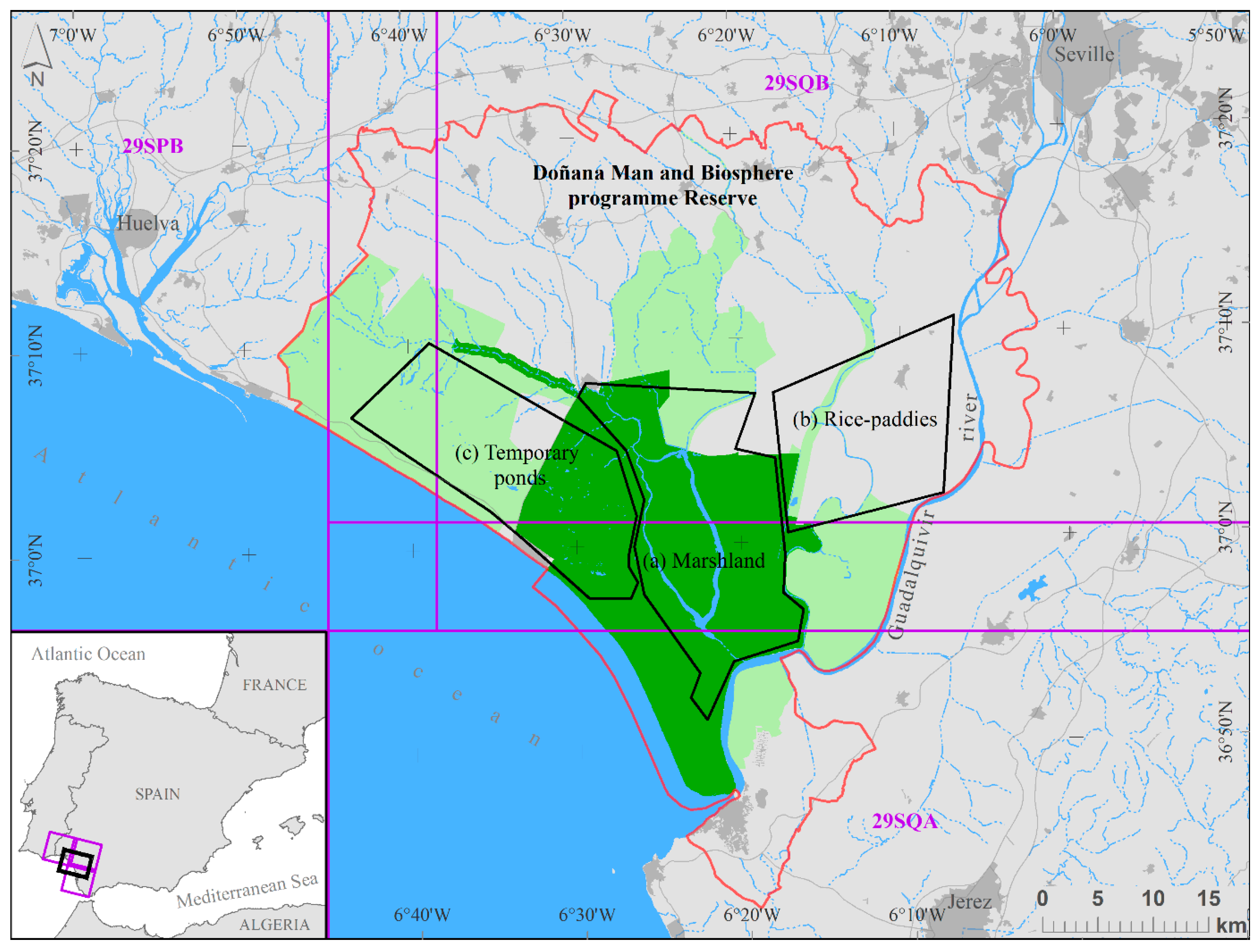
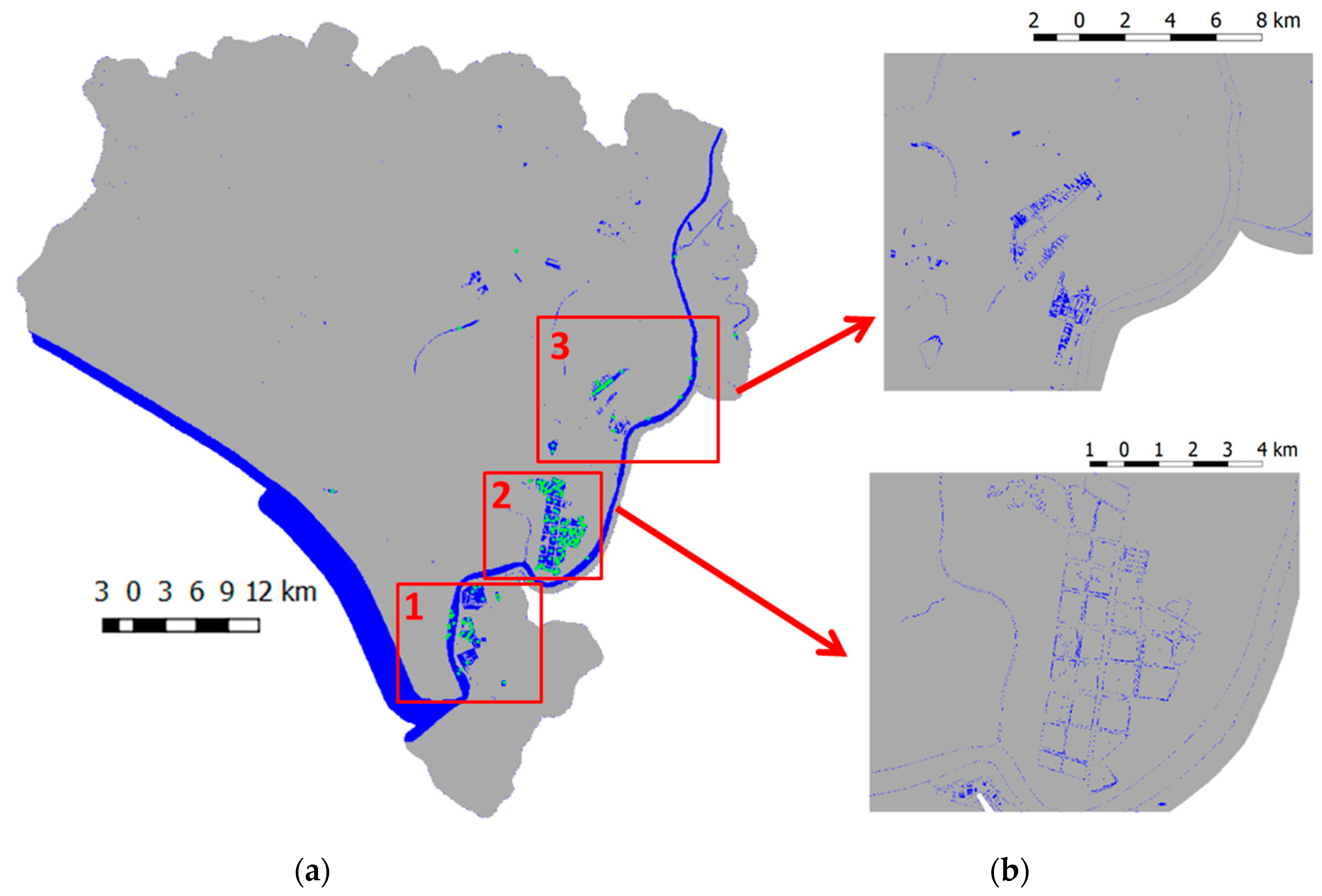
2.1. Study Area

The Doñana wetlands extend over 108,429 ha at the estuary of the Guadalquivir River in Southwest Spain [31] (Figure 1). The former vast natural marshes (more than 100,000 ha) that covered both sides of the Guadalquivir River were reduced to 32,000 ha on the western bank of the river. Large areas were completely drained for extensive agriculture, and others were transformed into saltpans, rice-fields and fish farms [32]. These man-made habitat changes resulted in a complex mosaic of diverse aquatic habitats of different sizes and water depths, ranging from natural to artificial wetlands, from fresh to hypersaline and from ephemeral to permanent water [33]. The Doñana climate is Mediterranean sub-humid with temperate and rainy autumns and winters and hot and dry summers. The average annual rainfall is 550 mm, with an interannual variation ranging from 170 mm (2004–2005) to 1000 mm (1995–1996). A diagram of the long-term average rainfall over the study area is provided in Díaz-Delgado et al. [2]. Rainfall occurs mainly from October–April, and the dry season is between May and September. Variable rainfall floods Doñana marshes, forming a wide floodplain that dries up during summer. Flooded areas are variable in depth, turbidity and vegetation cover, being driven mainly by the amount and seasonal pattern of rainfall. These seasonal marshes constitute the largest flooded surface in the Doñana wetlands and are breeding and wintering habitat for many species of European water birds [2]. On the aeolian sand deposits that close the mouth of the Guadalquivir River, there is an extensive system of temporary ponds [34]. Ponds range from small ephemeral pools that flood for a few days or weeks in rainy years to a few large permanent fresh-water lakes. Rice-paddies, created on top of the former natural marshes, are artificially flooded depending on rice cultivation needs and water available for cultivation. These areas, together with salt pans and aquaculture ponds, constitute an extensive system of artificial wetlands in the Doñana protected area that also provide refuge habitat for many species or water birds, especially when natural wetlands are dry [35].

2.2. Satellite Imagery

All available cloud-free Sentinel-2 (S2) products for Doñana National Park from 19 December 2015–20 August 2017 were downloaded from the Copernicus European Space Agency (ESA) hub. In total, S2 products from 23 different dates were downloaded (see

Table 1. Dates of S2 acquisition. ^(L) Denotes S2 images coinciding with Landsat images; green and yellow shading shows the presence of emergent vegetation covering marshland and rice-paddies, respectively.

Cycle	September	October	November	December	January	February	March	April	May	June	July	August
2015–2016				19 29 (L)		17	8			6 (L)	16 (L) 26	5 25 (L)
2016–2017	4 24	4 (L)		23 (L)	12			2 12	2	1 (L)	11 21 31	20
										11

).

Preprocessing of Sentinel-2 Data

S2 data Level-2A products are generated using the Sentinel-2 Level-2A Prototype Processor (Sen2Cor) software [36]. Sen2Cor pre-processes Level-1C (L1C) Top-Of-Atmosphere (TOA) image data and performs the tasks of atmospheric correction and subsequent conversion into an ortho-image Level-2A (L2A) Bottom-Of-Atmosphere (BOA) reflectance product. The preprocessing is performed per tile. The shapefile containing the boundaries of Doñana Biosphere Reserve comprises three different tiles (namely the 29SQA, 29SQB and 29SPB S2 tiles; see Figure 1), where brightness may differ from tile to tile. Therefore, L2A reflectance tile products are mosaicked and clipped to the limits of the shapefile. Mosaicking is performed independently for each S2 band by matching the histogram of each input tile’s band to the histogram of a source tile’s band. The center tile (29SQB) is assumed to be the source tile, since it covers the marshes and the majority of the study area, and at the same time, it overlaps with both the 29SQA and 29SPB tiles. The match tables are generated based on the overlapping portions of the 29SQA and 29SPB tiles’ bands with the 29SQB tile bands. The mosaicking and the clipping are conducted in ERDAS IMAGINE’s MosaicPro tool [37].

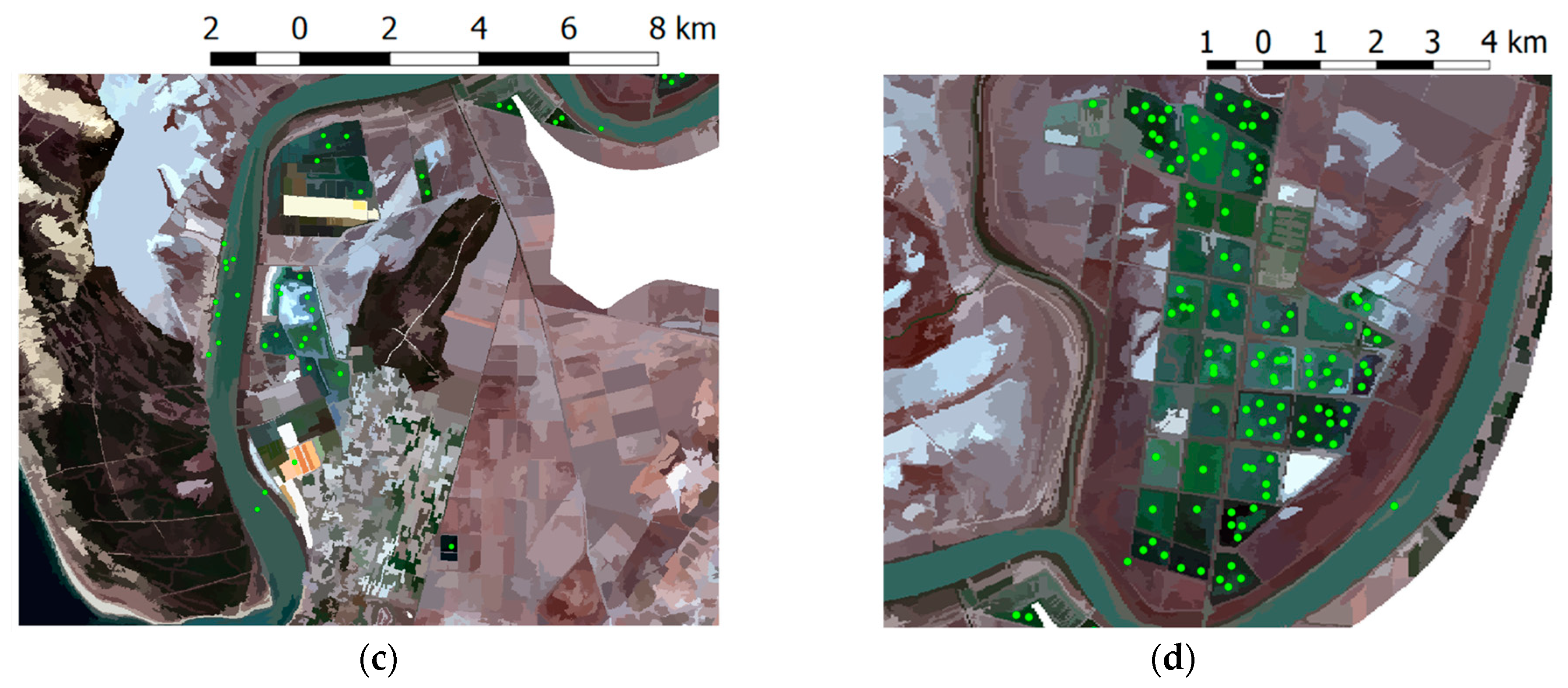
2.3. Ground Truth Data

Inundation maps of the Doñana area with 30-m pixel resolution, which are generated from Landsat satellite data and provided by the Doñana Biological Station (EBD), are used as ground truth data to evaluate the performance of the unsupervised and supervised approaches. The approach used for the generation of the Landsat inundation maps is described in detail in Díaz-Delgado et al. [2] and relies on Landsat band 5 (Short-Wave Infrared (SWIR)). Resulting inundation maps have a coarser spatial resolution than the product of the Sentinel-2 that is evaluated in this study. However, these inundation maps cover the whole area, are reliable and have been extensively tested with field data collected simultaneously with satellite overpasses. The use of these inundation maps, which are regularly produced by the EBD team, allowed testing the unsupervised approach on 7 different dates of S2 image acquisitions coinciding with the Landsat ones (denoted with (L) in Table 1).

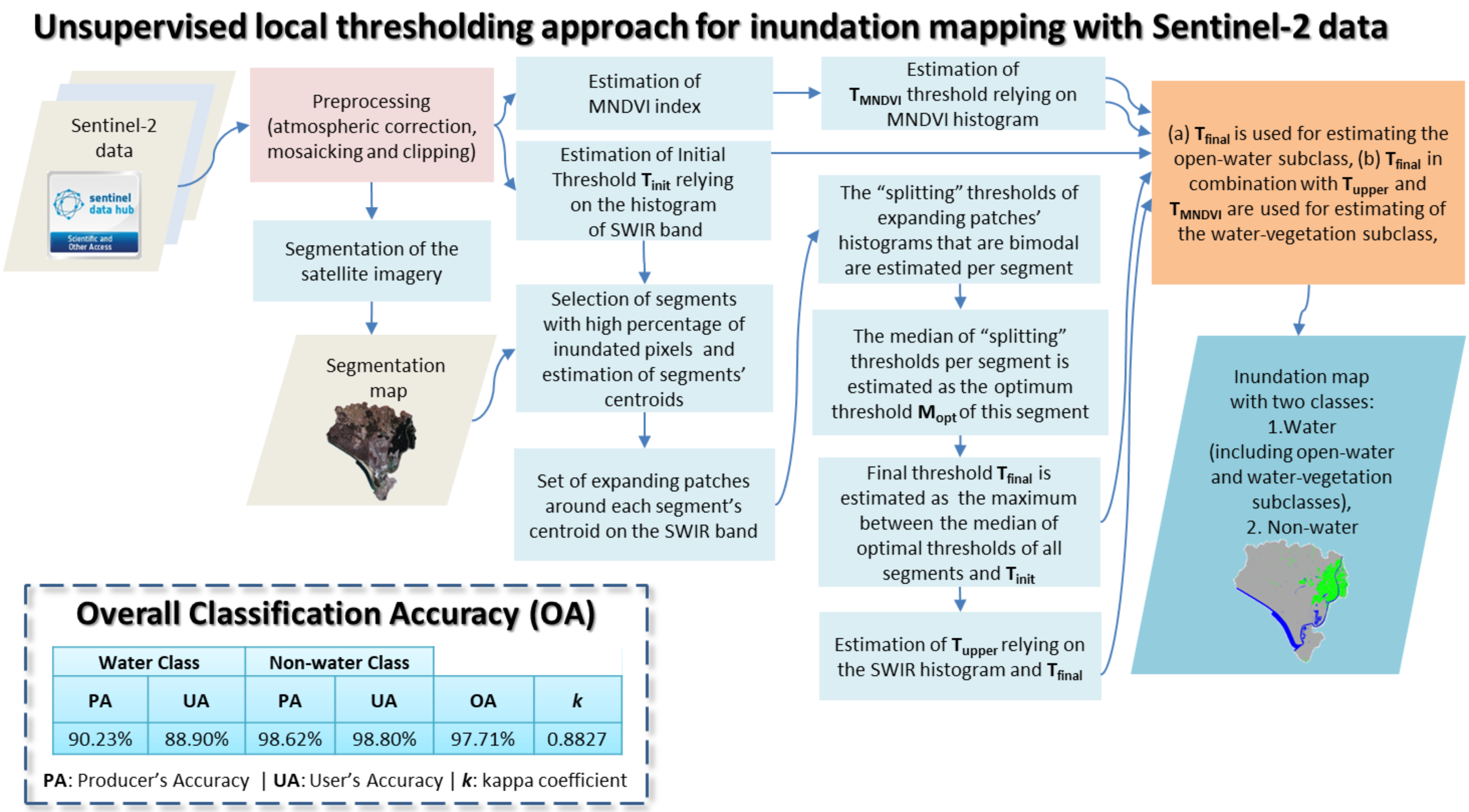
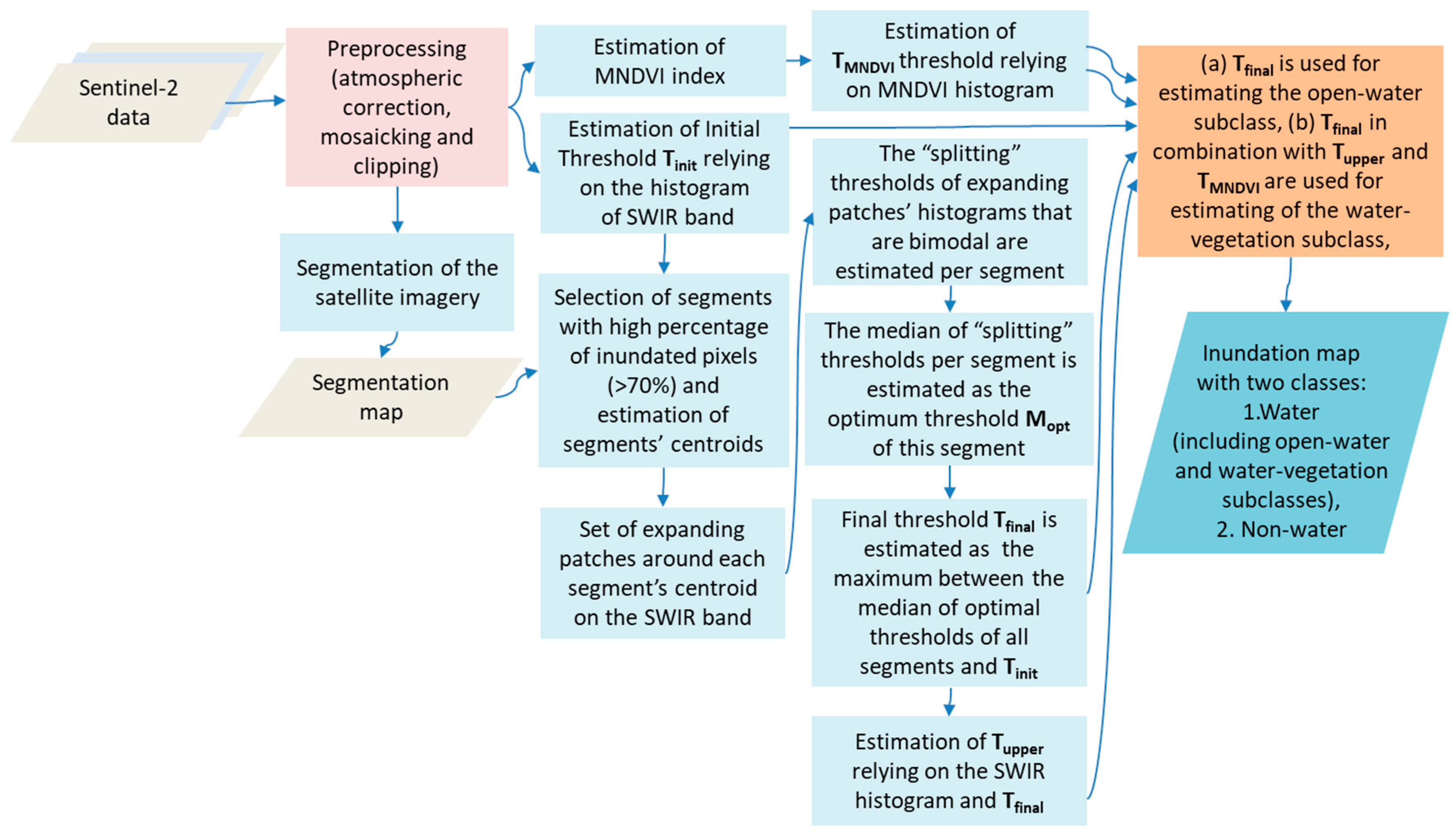
2.4. Unsupervised Approach

An unsupervised approach was developed, with the objective to be easily transferred and applied to other study areas without the need for ground truth information coincident with the satellite overpass. The performance of the unsupervised approach is compared to that of a supervised approach that uses as ground truth Landsat inundation maps developed by the EBD team. Both approaches are validated against the inundation map of the same date derived from Landsat.

The unsupervised approach estimates open-water and water-vegetation subclasses, which are then merged into the water class for validation purposes (see Figure 2). This way, usual wetland conditions, which allow for the presence of water over land at varying depths, where emergent vegetation may be absent, sparse or dense, are treated.

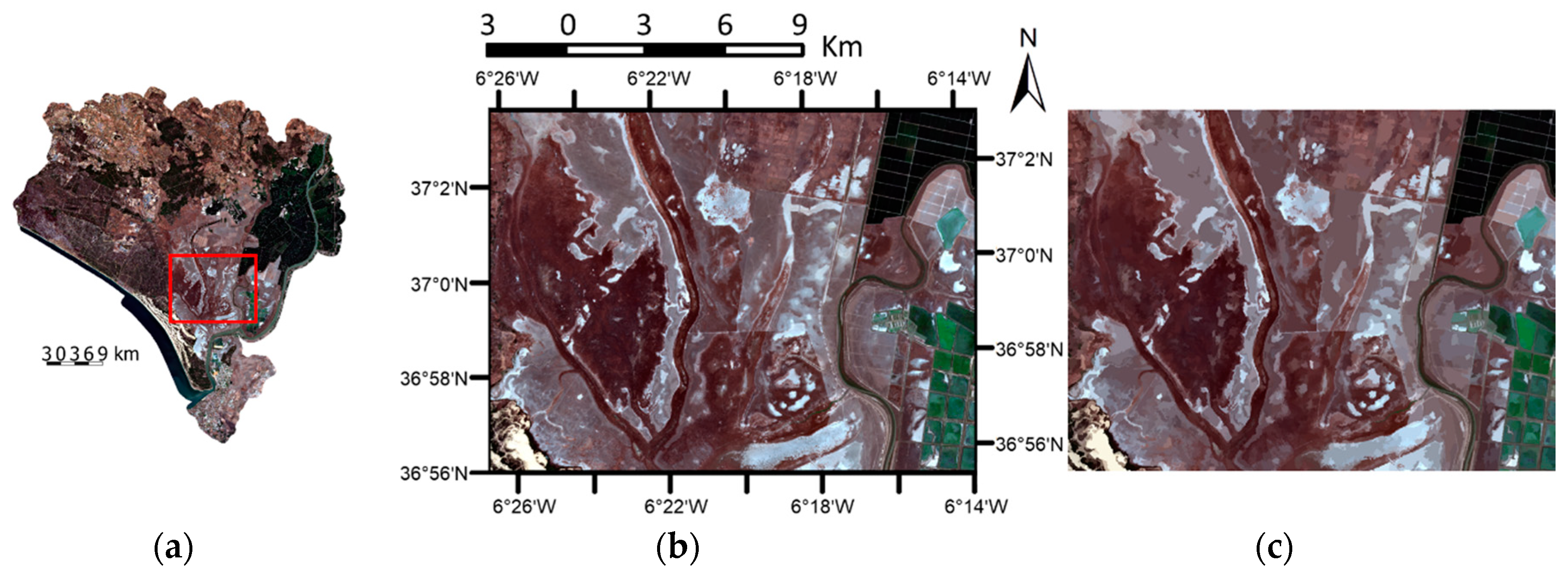
2.4.1. Segmentation of the Satellite Image

An initial step of the unsupervised approach is the segmentation of the satellite image into non-overlapping regions by utilizing the mean-shift segmentation algorithm [38], which relies on color and edge information. The input to the segmentation algorithm is a false color image composed of three channels. Band 2 (BLUE), Band 3 (GREEN) and Band 4 (RED) are selected as the three input channels due to their 10-m spatial resolution, which allows a more accurate segmentation of the satellite image, compared to the case of selecting as input other S2 bands, which have a resolution equal to or greater than 20 m, with the exception of Band 8, which has 10-m resolution. The intensity of each selected band is normalized to the range [0, 255]. The minimum and the maximum intensity values, on which each band is normalized, represent the intensity percentile range from 1–99%. Outlier intensities are set to 0 or 255 if they are less or greater than the minimum or maximum value, respectively. The parameters used for the mean-shift segmentation are the segmentation spatial radius h_s, which is set to h_s = 3, and the segmentation feature space radius h_r, which is set to h_r = 3. The selection of these strict values ensures that the segmentation map will be of high reliability, meaning that most likely, a segment will be comprised of pixels belonging to surfaces with similar spectral behavior. The latter fact is verified also in [39,40]. An example for performing mean-shift segmentation to the blue, green and red bands of Sentinel-2 (S2) data acquired on 20 August 2017 is given in Figure 3. The segmentation map is utilized for the selection of segments with a high percentage of inundated pixels. Therefore, it is important to confirm experimentally that small variations of the mean-shift segmentation parameters that adjust the segmentation map do not significantly affect the performance of the unsupervised approach. Relevant experimental results are given in Section 2.4.3.

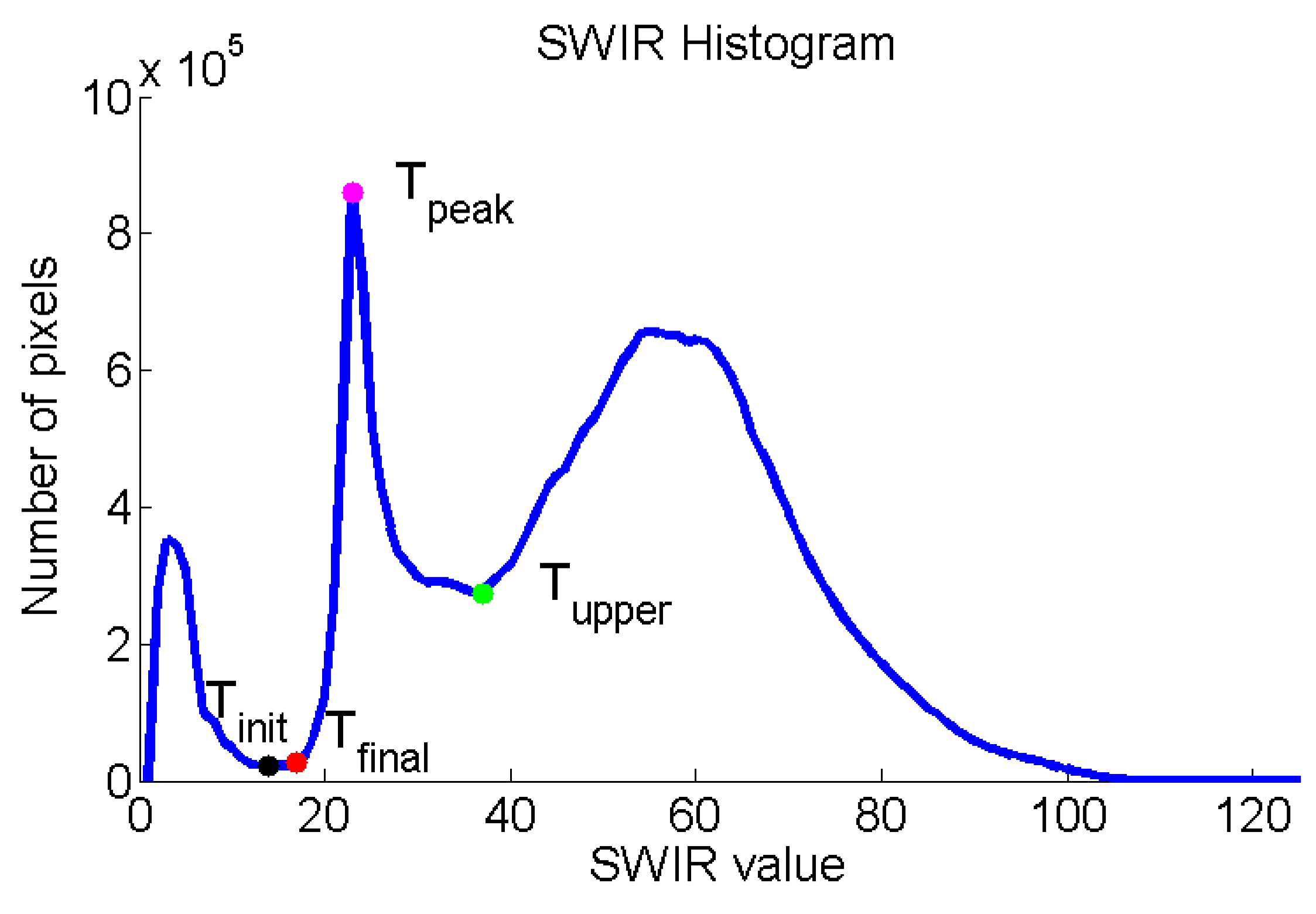
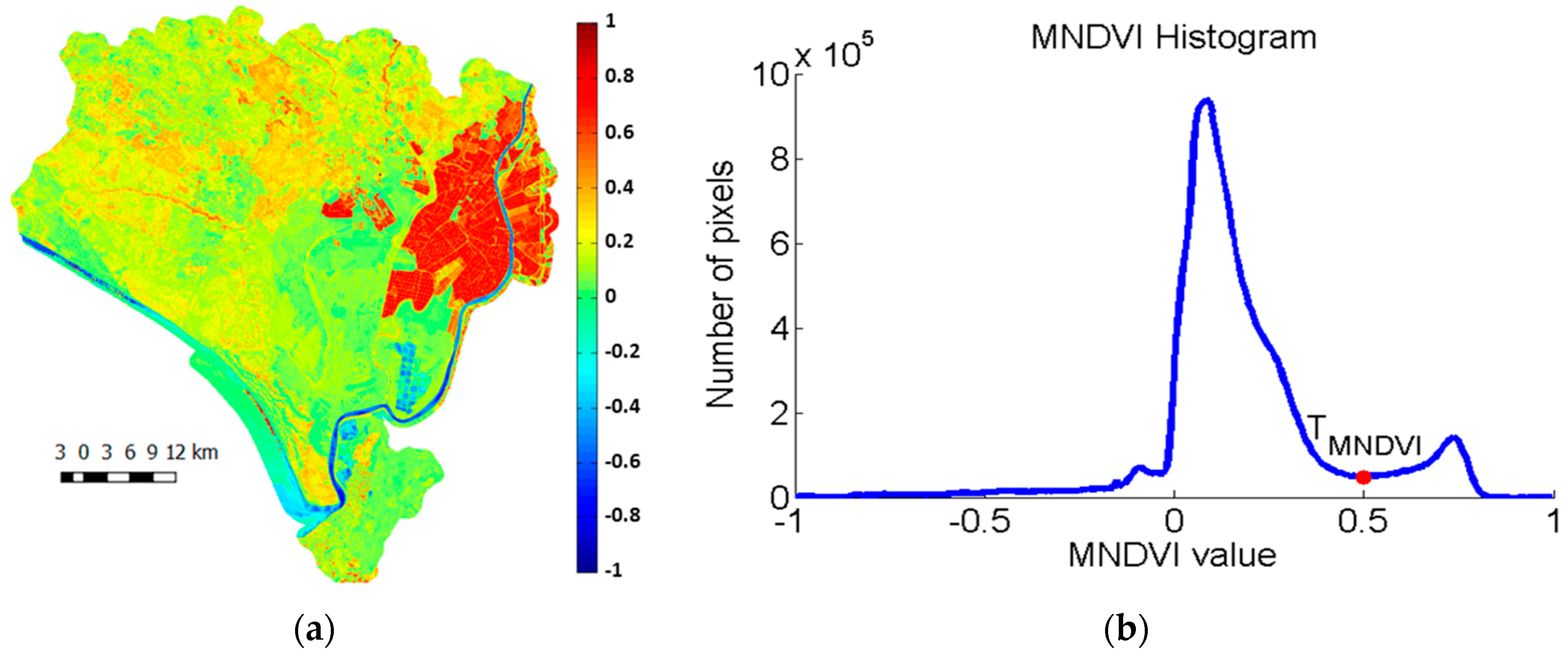
2.4.2. Mapping of the Open-Water Subclass

Several approaches in the literature aiming to identify shallow inundated wetland areas rely on the low reflectance values of water in the SWIR band, since it is less sensitive to sediment-filled waters and therefore more suitable for delineating the boundaries between water and dry ground in shallow wetland areas [2,41]. Hence, the unsupervised approach is based on the selection of a threshold on SWIR (Band 11) of S2. The SWIR band is normalized to the range of [0, 255] before using it in the unsupervised approach.

The histogram of the SWIR band is used to estimate an initial threshold ${\mathbf{T}}_{\mathbf{init}}$ separating inundated (low reflectance) from non-inundated pixels (medium to high reflectance). ${\mathbf{T}}_{\mathbf{init}}$ is the SWIR value, for which the first deep valley of the SWIR histogram is detected (see Figure 4). If a pixel p has $\mathrm{SWIR}(\mathbf{p})<{\mathbf{T}}_{\mathbf{init}}$, it is denoted as inundated, otherwise as non-inundated. Therefore, an initial inundation map is generated using ${\mathbf{T}}_{\mathbf{init}}$ (see Figure 5a). Based on this inundation map, segments ${\mathbf{G}}_{\mathbf{m}}$, where $\mathbf{m}\in \left\{1,2,\dots ,\mathbf{M}\right\}$, having a large percentage of inundated pixels (>70%) are selected and their corresponding centroids ${\mathbf{C}}_{\mathbf{m}}$ are estimated (green dots in Figure 5a). Sea segments are not considered for estimating centroids. The subsets of the mean-shift segmentation map corresponding to Subsets 1 and 2 of Figure 5a and their corresponding centroids are visualized in Figure 5c,d.

Around each ${\mathbf{C}}_{\mathbf{m}}$, square patches ${\mathbf{p}}_{\mathbf{m}}^{\mathbf{k}}$ of different window sizes are centered. The window size in pixels is given by $[20\cdot \mathbf{k}\times 20\cdot \mathbf{k}], \mathrm{where} \mathbf{k}=1, 2, \dots , 20$. Each patch’s histogram is checked first for bimodality (double peaked), so that it is certain that it contains both inundated and non-inundated pixels. The splitting threshold $f_{opt}^{\mathbf{k}}$ is estimated relying on the Minimum Cross Entropy Thresholding algorithm (MCET) [30].

The median of all expanding patches’ optimal thresholds $\underset{\mathbf{k}=1, 2, \dots , 20}{\mathrm{median}}(f_{opt}^{\mathbf{k}})$ is estimated as the optimal threshold $f_{opt}^{\mathbf{m}}$ corresponding to the segment ${\mathbf{G}}_{\mathbf{m}}$. The rationale behind using expanding patches is to make the estimation of the optimal threshold more robust, since it is estimated relying on multiple splitting thresholds. Then, the median of selected segments’ optimal thresholds is estimated as: ${\mathbf{M}}_{\mathbf{opt}}=\underset{\mathbf{m}=1,2,\dots ,\mathbf{M}}{\mathrm{median}}(f_{opt}^{\mathbf{m}})$. The median is considered, instead of the mean, for the estimation of ${\mathbf{M}}_{\mathbf{opt}}$, since it is less sensitive to outlier values.

The final threshold ${\mathbf{T}}_{\mathbf{final}}$, discriminating the open-water subclass, is estimated as the maximum value between ${\mathbf{M}}_{\mathbf{opt}}$ and ${\mathbf{T}}_{\mathbf{init}}$, i.e., $\max \left({\mathbf{M}}_{\mathbf{opt}},{\mathbf{T}}_{\mathbf{init}}\right)$, in order to account at the same time for both the specificities of the intensively inundated subset areas and the whole area spectral behavior. Pixels p with $\mathrm{SWIR}(\mathbf{p})<{\mathbf{T}}_{\mathbf{final}}$ are assumed to belong to the open-water subclass. In Figure 5b are depicted, for Subset Areas 2 and 3 of Figure 5a, the additional water pixels identified in the open-water subclass map compared to the initial inundation map.

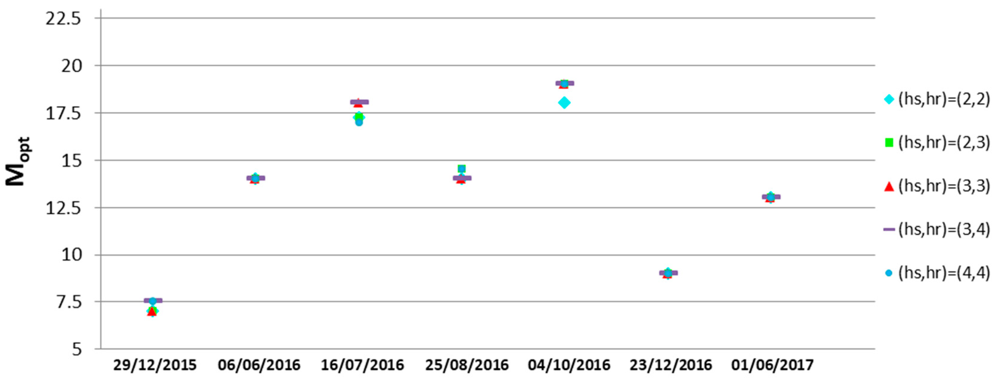
2.4.3. Testing of Mean-Shift Segmentation Parameters

The mean-shift segmentation map is exploited for segmenting the satellite image into non-overlapping regions (see Section 2.4.1). Therefore, it is important to verify that variations to the selected parameters (h_s,h_r) = (3,3) do not significantly affect the estimation of ${\mathbf{M}}_{\mathbf{opt}}$. The additional sets of tested mean-shift parameters are (h_s,h_r) = (2,3), (h_s,h_r) = (3,3), (h_s,h_r) = (3,4) and (h_s,h_r) = (4,4). The points in Figure 6 show for the 7 dates that S2 and Landsat overpasses coincide (see Table 1) and for 5 different selections of (h_s,h_r), the estimated ${\mathbf{M}}_{\mathbf{opt}}$. It is deduced that the influence of the variation of the segmentation parameters on the ${\mathbf{M}}_{\mathbf{opt}}$ estimation is negligible, since most values per date coincide or are very close.

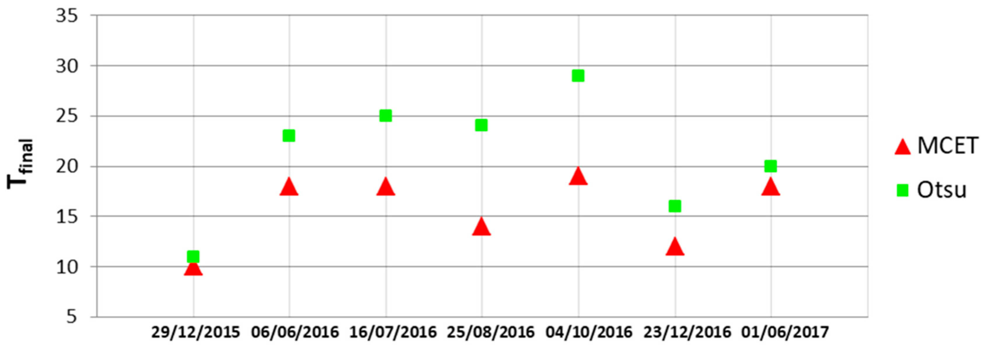
2.4.4. Effect of an Alternative Algorithm for Estimating Splitting Thresholds

A prevalent method for estimating an optimum threshold separating two classes is the Otsu method [21]. This method has been used in multiple approaches in the literature aiming at separating pixels into inundated and non-inundated classes [10,22,23,24,42]. In this experiment, MCET is replaced by the Otsu method, while the rest of the steps of the unsupervised approach are kept the same. The points in Figure 7 show the estimated ${\mathbf{T}}_{\mathbf{final}}$ for 7 dates by the two methods. The derived ${\mathbf{T}}_{\mathbf{final}}$ is always greater when using the Otsu method. The inundation maps generated relying on the use of MCET or the Otsu method are validated in Section 3.2, and the results suggest the use and better fit of the MCET method in the presented unsupervised methodology.

2.4.5. Mapping of the Water-Vegetation Subclass

There are areas where water may be covered by emergent dense vegetation. The SWIR value of the pixels in these areas is higher compared to the SWIR values of the pixels having water or water with sparse vegetation belonging to the open-water class. A threshold ${\mathbf{T}}_{\mathbf{upper}}$, which is the SWIR value for which the valley right after the first valley is detected in the SWIR histogram (see Figure 4), is assumed to be the upper threshold for pixels comprising areas of water covered by dense vegetation. However, at the same time, it is has to be ensured that vegetation is present. To identify the vegetated areas, a Modified Normalized Difference Vegetation Index (MNDVI) (see Figure 8a) is estimated, using Band 7 and Band 5 of S2 (see Table 3), and an MNDVI threshold ${\mathbf{T}}_{\mathbf{MNDVI}}$ that should be over 0.4 is selected based on a trial and error process for the area. Specifically, ${\mathbf{T}}_{\mathbf{MNDVI}}$ is set equal to the MNDVI value, for which the first valley in the part of the histogram with MNDVI values over 0.4 is detected (see Figure 8b). A pixel p is assumed to belong to the water-vegetation subclass, when the following two conditions are satisfied:

$$\{\begin{array}{l}{\mathbf{T}}_{\mathbf{final}}<\mathrm{SWIR}(\mathbf{p})<{\mathbf{T}}_{\mathbf{upper}}\\ \mathrm{MNDVI}(\mathbf{p})>{\mathbf{T}}_{\mathbf{MNDVI}}\end{array},$$

(1)

Pixels of the water-vegetation subclass are demonstrated in the map of Figure 9a. Evidently, the water-vegetation subclass is mainly detected in the upper right area of the map, where the rice-paddies are located. These results comply with the growing cycle of rice, since the rice grows during the summer period in Doñana and at the same time the paddies are flooded [43]. MNDVI is preferred to the NDVI index (its formula is given in Table 3), since the use of NDVI causes the appearance of false positives in areas where water vegetation pixels are not expected, such as the areas enclosed in the red oval in Figure 9b (mainly vegetation inside sand dunes). The latter reveals that the higher spatial resolution of S2 Bands 4 and 8, used for calculating NDVI, is not that reliable as the narrow spectral width of S2 Bands 5 and 7, used for calculating MNDVI.

Supplementary (Supplementary S1) gives a sensitivity analysis of the unsupervised approach. The first part, entitled “1. Estimation of ${\mathbf{T}}_{\mathbf{init}}$”, describes how underestimation of ${\mathbf{T}}_{\mathbf{init}}$ can be prevented, while the second part, entitled “2. Deviation from the proposed unsupervised approach”, describes how the methodology proceeds when the water-vegetation subclass is not present.

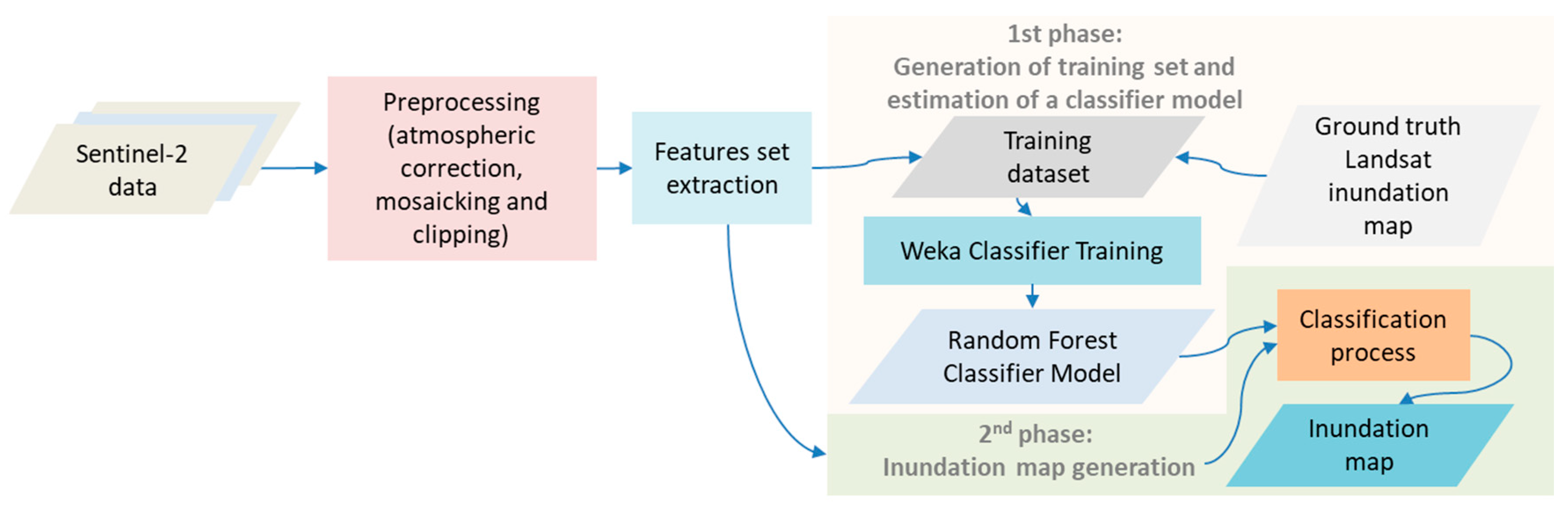
2.5. Supervised Approach

The 1st phase of the supervised approach (Figure 10) is to generate a training set composed of sample points for each one of the 7 different S2 acquisition dates having simultaneous Landsat overpasses (see Table 1) and then training a classifier model per date. For each sample point, a number of features, including S2 bands and indices, is estimated. Details on the S2 bands used and the derived indices are given in

Table 2. Details on the S2 bands used.

Setinel-2 Bands	Resolution
Band 2 (Blue); Band 3 (Green); Band 4 (Red); Band 8 (NIR)	10 m
Band 5 (Vegetation Red Edge); Band 6 (Vegetation Red Edge); Band 7 (Vegetation Red Edge); Band 8A (Narrow NIR); Band 11 (SWIR); Band 12 (SWIR) (upscaled to 10m relying on nearest-neighbors)	20 m

and

Table 3. Details on the derived indices.

Index Name and Abbreviation	Equation
Normalized Difference Water Index (NDWI)	(Band 3 − Band 8)/(Band 3 + Band 8)
Modified NDWI (MNDWI)	(Band 3 − Band 11)/(Band 3 + Band 11)
Normalized Difference Vegetation Index (NDVI)	(Band 8 − Band 4)/(Band 8 + Band 4)
Modified Normalized Difference Vegetation Index (MNDVI)	(Band 7 − Band 5)/(Band 7 + Band 5)

, respectively.

NDWI, MNDWI and NDVI are commonly suggested in the literature for water detection (e.g., by [44,45]). MNDVI is additionally used in the supervised approach, since it has been used in the unsupervised approach. The sampling of the points on the S2 images is regular, and one per five pixels is sampled for the water class, while one per fifteen pixels is sampled for the non-water class. The same sampling frequency is applied to both horizontal and vertical axis. Per sample point, the features given in Table 2 and Table 3 are estimated, while the class is derived from the Landsat inundation map that is overlaid on the S2 image. Since the date of S2 acquisition coincides with the date of the Landsat inundation map, it is ensured that the sample class can be reliably derived. The average number of training samples of the 7 training sets is 267.862, with 160.055 of them corresponding to the water class and the rest 107.807 to the non-water class.

The training dataset of each date is then loaded into the WEKA open source machine learning software [46] in order to train a Random Forest (RF) classifier, which is an ensemble of trees [47], per date. A 10-fold cross-validation is performed, i.e., the training dataset is randomly partitioned into 10 subsets of equal size, where a single subset is retained as the validation data for testing the model, and the remaining 9 subsets are used as training data. The cross-validation process is repeated 10 times, with each of the 10 subsets used exactly once as the validation data, and the 10 results are averaged to produce a single estimation. At the same time, the RF parameters were set to default (e.g., 100 trees). In this way, an RF model is generated per date. This is then applied (2nd phase in Figure 10) to the features calculated for the pixels of the S2 image acquired at the same date, in order to classify the image into water and non-water areas. On average, the time required to train the model, estimate the features and perform the classification per date is about 4 h and 20 min on a PC with an i7 CPU at 3.4 GHz and 128 GB of RAM. In comparison, the time required for the execution of the unsupervised methodology for these dates ranged from 22–37 min.

3. Results

3.1. Accuracy Assessment Results for S2 and Landsat Coincident Overpasses

The inundation maps produced on 20 August 2017 by the unsupervised and supervised approaches are depicted in Figure 11a,b, respectively.

The unsupervised and supervised approaches use as input S2 bands with a resolution equal to 10 m or 20 m, allowing the generation of inundation maps with a resolution of 10 m, while the Landsat inundation maps used as ground truth data have a resolution of 30 m. Therefore, the lower spatial resolution of Landsat images induces an amount of error in the accuracy assessment of the presented approaches, since Landsat inundation maps, which are assumed to be ground truth maps, lack accuracy in the transition zones between water and non-water regions compared to the S2 inundation maps. Additionally, the higher resolution of the S2 estimated inundation maps allows for the detection of smaller areas covered by water that probably cannot be identified in Landsat inundation maps. Figure 12 shows side-by-side subparts of the unsupervised and the Landsat estimated inundation maps on 25 August 2016, where differences are evident.

In order to compensate for the uncertainty caused in the validation due to the lower spatial resolution of the Landsat-derived inundation maps, two validation results are presented: in Situation (i), boundary regions between inundated and non-inundated pixels are excluded from the accuracy estimation, and in Situation (ii), boundary regions are included. Pixels in the area corresponding to sea coastal waters are not taken into consideration to obtain unbiased classification results. Landsat inundation maps are comprised of the water class and the non-water class. The boundary regions in the Landsat mask are comprised of pixels including in their eight closest-neighbor pixels at least one pixel of a different class. Figure 13a shows a map including the boundary regions and Figure 13b a zoomed region of it.

Summarizing, the validation with Landsat ground truth data is estimated for two situations: (i) Excluding boundary Ambiguous Pixels (EAP) and (ii) Including boundary Ambiguous Pixels (IAP), in the accuracy estimation. The results for EAP situation are given in

Table 4. Part A and Part B show for the complete area the accuracy assessment results for the unsupervised and supervised approaches, respectively.

Part A		Unsupervised: Complete Area
	Date	29 December 2015		6 June 2016		16 July 2016		25 August 2016		4 October 2016		23 December 2016		1 June 2017
Class		PA	UA	PA	UA	PA	UA	PA	UA	PA	UA	PA	UA	PA	UA
Water class		91.34%	93.41%	93.21%	94.46%	90.03%	68.98%	94.77%	70.79%	90.76%	97.16%	85.10%	95.82%	92.49%	95.21%
Non-water class		99.20%	98.93%	99.38%	99.23%	96.79%	99.19%	97.05%	99.60%	99.93%	99.75%	98.94%	95.86%	99.10%	98.55%
OA		98.33%		98.75%		96.30%		96.89%		99.68%		95.86%		98.02%
k		0.9143		0.9313		0.7613		0.7939		0.9369		0.8753		0.9266
Part B		Supervised: Complete Area
	Date	29 December 2015		06 June 2016		16 July 2016		25 August 2016		4 October 2016		23 December 2016		1 June 2017
Class		PA	UA	PA	UA	PA	UA	PA	UA	PA	UA	PA	UA	PA	UA
Water class		99.26%	91.58%	99.05%	92.85%	98.81%	93.02%	98.24%	84.90%	98.30%	95.78%	98.61%	92.23%	99.38%	93.98%
Non-water class		98.87%	99.91%	99.13%	99.89%	99.41%	99.90%	98.68%	99.87%	99.88%	99.95%	97.62%	99.59%	98.76%	99.88%
OA		98.91%		99.12%		99.37%		98.65%		99.84%		97.84%		98.86%
k		0.9465		0.9536		0.9548		0.9036		0.9694		0.9391		0.9592

,

Table 5. Part A and Part B show for the marshland the accuracy assessment results for the unsupervised and supervised approaches, respectively.

Part A		Unsupervised: Marshland
	Date	29 December 2015		6 June 2016		16 July 2016		25 August 2016		4 October 2016		23 December 2016		1 June 2017
Class		PA	UA	PA	UA	PA	UA	PA	UA	PA	UA	PA	UA	PA	UA
Water class		91.48%	99.36%	91.07%	99.73%	88.74%	82.41%	90.16%	54.68%	92.83%	95.97%	92.84%	99.98%	88.32%	99.93%
Non-water class		99.98%	99.75%	99.93%	97.34%	99.92%	99.95%	99.90%	99.99%	99.99%	99.99%	99.94%	79.79%	99.95%	90.92%
OA		99.74%		97.85%		99.87%		99.89%		99.99%		94.40%		94.59%
k		0.9512		0.9383		0.8540		0.6802		0.9438		0.8508		0.8902
Part B		Supervised: Marshland
	Date	29 December 2015		6 June 2016		16 July 2016		25 August 2016		4 October 2016		23 December 2016		1 June 2017
Class		PA	UA	PA	UA	PA	UA	PA	UA	PA	UA	PA	UA	PA	UA
Water class		98.59%	92.76%	99.26%	97.95%	96.53%	95.74%	97.56%	87.25%	98.65%	77.81%	99.01%	98.52%	99.24%	98.70%
Non-water class		99.77%	99.96%	99.37%	99.77%	99.98%	99.99%	99.98%	99.99%	99.98%	99.99%	94.73%	96.45%	98.88%	99.35%
OA		99.74%		99.34%		99.97%		99.98%		99.98%		98.07%		99.05%
k		0.9545		0.9817		0.9612		0.9611		0.8699		0.9435		0.9809

,

Table 6. Part A and Part B show for the rice-paddies the accuracy assessment results for the unsupervised and supervised approaches, respectively.

Part A		Unsupervised: Rice-Paddies
	Date	29 December 2015		6 June 2016		16 July 2016		25 August 2016		4 October 2016		23 December 2016		1 June 2017
Class		PA	UA	PA	UA	PA	UA	PA	UA	PA	UA	PA	UA	PA	UA
Water class		92.08%	99.97%	94.62%	99.58%	86.34%	70.44%	95.90%	76.23%	47.30%	98.80%	82.26%	99.98%	95.15%	99.94%
Non-water class		99.95%	86.49%	99.75%	96.80%	71.44%	86.90%	75.36%	95.70%	99.99%	99.69%	99.95%	65.84%	99.87%	90.33%
OA		94.73%		97.80%		78.00%		84.64%		99.69%		86.77%		96.62%
k		0.8863		0.9529		0.5642		0.6967		0.6384		0.7024		0.9236
Part B		Supervised: Rice-Paddies
	Date	29 December 2015		6 June 2016		16 July 2016		25 August 2016		4 October 2016		23 December 2016		1 June 2017
Class		PA	UA	PA	UA	PA	UA	PA	UA	PA	UA	PA	UA	PA	UA
Water class		99.63%	98.98%	99.07%	97.84%	98.87%	98.00%	97.85%	87.23%	89.18%	74.10%	98.71%	98.39%	99.69%	99.51%
Non-water class		97.98%	99.27%	98.66%	99.42%	98.41%	99.10%	88.19%	98.03%	99.81%	99.94%	95.27%	96.21%	98.92%	99.31%
OA		99.08%		98.81%		98.61%		92.56%		99.75%		97.84%		99.45%
k		0.9792		0.9749		0.9719		0.8513		0.8082		0.9429		0.9871

,

Table 7. Part A and Part B show for the temporary ponds the accuracy assessment results for the unsupervised and supervised approaches, respectively.

Part A		Unsupervised: Temporary Ponds
	Date	29 December 2015		6 June 2016		16 July 2016		25 August 2016		4 October 2016		23 December 2016		1 June 2017
Class		PA	UA	PA	UA	PA	UA	PA	UA	PA	UA	PA	UA	PA	UA
Water class		93.03%	83.21%	94.25%	65.53%	96.58%	33.58%	94.76%	23.40%	98.37%	12.25%	79.12%	89.16%	92.24%	54.89%
Non-water class		99.99%	99.99%	99.95%	99.99%	99.90%	99.99%	99.93%	99.99%	99.92%	99.99%	99.99%	99.97%	99.90%	99.99%
OA		99.98%		99.95%		99.90%		99.93%		99.92%		99.95%		99.89%
k		0.8784		0.7729		0.4980		0.3751		0.2177		0.8382		0.6877
Part B		Supervised: Temporary Ponds
	Date	29 December 2015		6 June 2016		16 July 2016		25 August 2016		4 October 2016		23 December 2016		1 June 2017
Class		PA	UA	PA	UA	PA	UA	PA	UA	PA	UA	PA	UA	PA	UA
Water class		96.60%	55.82%	95.83%	60.11%	99.09%	33.33%	99.37%	21.36%	100%	10.29%	90.36%	58.10%	96.51%	59.70%
Non-water class		99.95%	99.99%	99.94%	99.99%	99.90%	99.99%	99.92%	99.99%	99.90%	100%	99.90%	99.99%	99.92%	99.99%
OA		99.95%		99.94%		99.90%		99.92%		99.90%		99.89%		99.91%
k		0.7073		0.7372		0.4984		0.3513		0.1864		0.7067		0.7373

and

Table 8. Combined accuracy assessment for all 7 dates per approach and examined study area.

		Water Class		Non-Water Class
	Measure	PA	UA	PA	UA	OA	k
Approach and Study Area
1	Unsupervised (MCET): Complete area	90.23%	88.90%	98.62%	98.80%	97.71%	0.8827
2	Supervised: Complete area	98.90%	92.06%	98.96%	99.86%	98.95%	0.9477
3	Unsupervised: Marshland	91.14%	99.77%	99.95%	97.82%	98.18%	0.9413
4	Supervised: Marshland	99.10%	98.32%	98.96%	99.77%	99.48%	0.9839
5	Unsupervised: Rice-paddies	90.54%	92.09%	92.87%	91.46%	91.76%	0.8347
6	Supervised: Rice-paddies	99.07%	97.21%	97.39%	99.13%	98.19%	0.9639
7	Unsupervised: Temporary Ponds	89.67%	52.59%	99.94%	99.99%	99.93%	0.6626
8	Supervised: Temporary Ponds	95.04%	46.32%	99.92%	99.99%	99.91%	0.6224
9	Unsupervised (Otsu): Complete area	94.20%	76.49%	96.46%	99.27%	96.21%	0.8320

, while for the IAP situation, they are given in Supplementary (Supplementary S2). As expected, the accuracy results of EAP are superior to those of IAP. Accuracy differences between EAP and their corresponding IAP values indicate that part of the lack of agreement between the S2 and Landsat inundation maps is due to the lower resolution of the Landsat map. The accuracy estimation results include the estimation of Producer’s Accuracy (PA), User’s Accuracy (UA), Overall Accuracy (OA) and the kappa coefficient (k). The confusion matrices, based on which the results of Table 4, Table 5, Table 6, Table 7 and Table 8 are produced, are included in Supplementary (Supplementary S3). A detailed insight into the results is given in the following.

Table 4 presents the accuracy assessment for the complete buffered Biosphere Reserve area. Part A of Table 4 indicates that the PA of the water class is over 85.10% for all dates. The UA of the water class is low for two dates during the summer period, on 16 July 2016 (68.98%) and 25 August 2016 (70.79%), while for the rest of the dates, the UA is over 93.41%. On the other hand, Part B of Table 4 indicates that the PA and UA of the water class are over 98.24% and 84.90% for all dates, respectively. For both approaches, k is over 0.76. This shows that all classifications show “substantial” (0.61 ≤ k ≤ 0.80) or “almost perfect” (0.81≤ k ≤ 1) agreement between the observed and predicted classes according to [48].

Since the Doñana protected area includes three different types of wetlands, (a) seasonal marshland, (b) cultivated rice-paddies and (c) temporary ponds, the accuracy assessment results are presented separately for each type of wetland. The boundaries of the aforementioned wetland types are depicted in Figure 1.

Table 5 presents the accuracy assessment for the marshland area. Part A of Table 5 indicates that the PA of the water class is over 88.32% for all dates. The UA of the water class is low for one date during the summer period, on 25 August 2016 (54.68%), while for the rest of the dates, the UA is over 82.41%. On the other hand, Part B of Table 5 indicates that the PA and UA of the water class are over 96.53% and 77.81%, respectively. For the unsupervised approach, k is over 0.6802, while for the supervised one, k is over 0.8699.

Table 6 presents the accuracy assessment for the rice-paddies. Part A of Table 6 indicates that the PA of the water class is very low on 4 October 2016 (47.30%), while for the rest of the dates, it is over 82.26%. The UA of the water class is over 71.44%. On the other hand, Part B of Table 6 shows that the PA and UA of the water class are over 89.18% and 74.10%, respectively. For the unsupervised approach, k is over 0.5642, while for the supervised approach, k is over 0.8082.

Table 7 presents the accuracy assessment for the temporary ponds areas. Part A of Table 7 indicates that the PA is over 79.12%, while the UA ranges from 12.25–89.16%. Part B of Table 7 indicates that the PA ranges from 90.36–100%, while the UA ranges from 10.29–60.11%. For the unsupervised approach, k ranges from 0.2177–0.8784, while for the supervised approach, k ranges from 0.1864–0.7373. Evidently, there is a significant variation in the accuracy results, since the small size of the area covered by the temporary ponds may allow for the detection of small water-covered areas in S2 data, but not in Landsat data.

The average k of marshland, rice-paddies and temporary ponds for the unsupervised approach is 0.8726, 0.7664 and 0.6097, respectively, and for the supervised approach is 0.9504, 0.9308 and 0.5607, respectively. k values are lower in the temporary ponds and also somewhat lower in the rice-paddies compared to the marshland. The statistical relation between k and different factors, e.g., (a) type of wetland, (b) water covered area and (c) perimeter of water covered area, is also examined based on ANOVA (Analysis Of Variance). The ANOVA results (F = 3.853, p = 0.04048) indicate a significant relation between k and wetland type. Furthermore, from Part B of Table 4, Table 5, Table 6 and Table 7, it is found that for the supervised approach, the PA is higher than the UA for the water class and for all dates and examined areas, and this shows that the water area tends to be overestimated compared to Landsat reference maps. On the contrary, Part A of Table 4, Table 5, Table 6 and Table 7 demonstrates that for the unsupervised approach, there is no consistent tendency to overestimate or underestimate water coverage, since the PA can be increased or decreased compared to UA.

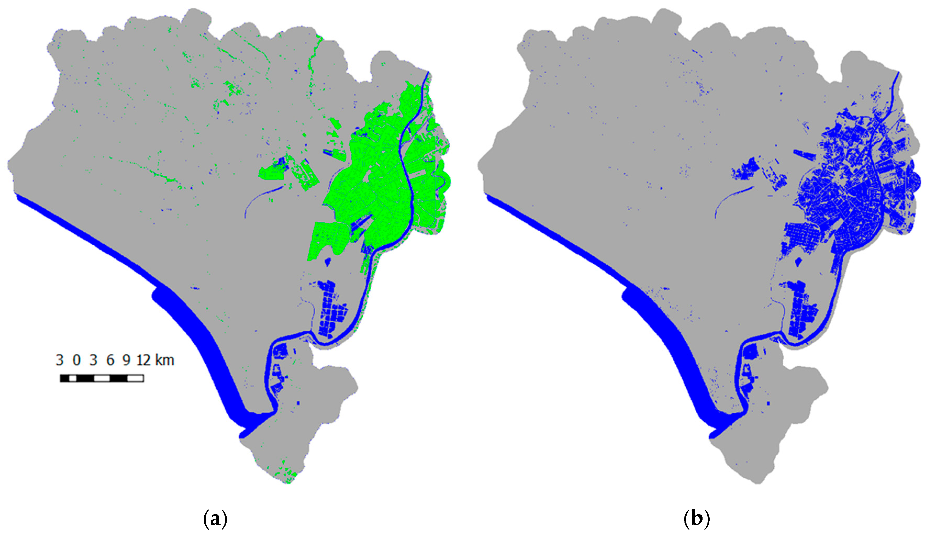
3.2. Combined Accuracy

The rows in Table 8 provide the PA, UA, OA and k, which are estimated when the number of true positive pixels of the water class, false positive pixels of the water class, true positive pixels of the non-water class and false positive pixels of the non-water class are added for all seven dates per approach and examined study area (information about the approach and the study area is given in the second column).

For the complete buffered Biosphere Reserve area, by comparing the first and second rows of Table 8, it is estimated that for the water class, the PA and the UA of the unsupervised approach are 8.67% and 3.16% lower than that of the supervised approach, respectively. k of the supervised approach is about 7.1% higher than the unsupervised approach. For the marshland area, by comparing the third and fourth rows of Table 8, it is estimated that for the water class, the PA of the unsupervised approach is 7.96% lower than that of the supervised approach. In contrast, the UA of the unsupervised approach is 1.45% higher than that of the supervised approach. k of the supervised approach is about 4.43% higher than the unsupervised approach. For the rice-paddies, by comparing the fifth and sixth rows of Table 8, it is estimated that for the water class, the PA and UA of the unsupervised approach are 8.53% and 5.12% lower than the supervised approach, respectively. k of the supervised approach is about 14.37% higher than the unsupervised approach. For the temporary ponds, by comparing seventh and eight rows of Table 8, it is estimated that for the water class, the PA of the unsupervised approach is 5.37% lower than the supervised approach. In contrast, the UA of the unsupervised approach is 6.27% higher than the supervised approach. k of the unsupervised approach is about 6.26% higher than the supervised approach. Summarizing the combined accuracy assessment results, the PA of the unsupervised approach is 5.37–8.67% lower than the supervised approach, while the UA of the unsupervised approach can be lower or higher than the supervised approach, with a fluctuation ranging from −5.12–6.27%. k is higher for the supervised approach for all study areas, except for the temporary ponds.

The ninth row of Table 8 provides PA, UA, OA and k derived from the inundation maps estimated for the complete area relying on the unsupervised approach and the Otsu method (see Section 2.4.4). The ninth row is compared to the first row to evaluate how the performance of the unsupervised approach is affected when the Otsu method is used instead of MCET for estimating splitting thresholds. Though, the PA of the unsupervised approach with MCET is 3.97% lower than the unsupervised approach with the Otsu method, and the UA of the unsupervised approach with MCET is 12.41% higher than UA of the unsupervised approach with the Otsu method. Additionally, when using the Otsu method in the unsupervised approach, the PA is significantly higher than the UA (the difference between them is 17.71%). On the contrary, when MCET is used in the unsupervised method, the difference between the PA and UA is limited to 1.33%. k is about 5.91% higher when using MCET than the Otsu method.

Taking into consideration the inundation maps, generated for all 23 dates given in Table 1, information about the statistics of the estimated ${\mathbf{T}}_{\mathbf{final}}$ and ${\mathbf{T}}_{\mathbf{upper}}$ can be obtained. The minimum, maximum and mean values of ${\mathbf{T}}_{\mathbf{final}}$ are 9, 31 and 15.174, respectively. While, the minimum, maximum and mean values of ${\mathbf{T}}_{\mathbf{upper}}$ are 29, 67 and 36.33, respectively. The mean ${\mathbf{T}}_{\mathbf{upper}}$ value is close to the minimum value, since only for one date, ${\mathbf{T}}_{\mathbf{upper}}$ is over 37 (i.e., 67). It has to be noted that ${\mathbf{T}}_{\mathbf{upper}}$ is estimated in nine out of 23 dates (these dates are shadowed with yellow in Table 1 and lie within the summer period), thus indicating the presence of the water-vegetation subclass.

3.3. Performance of the Unsupervised Approach in Marshland

Park managers of Doñana protected area have a special interest in estimating the hydroperiod in seasonal marshland, since this area is considered as Western Europe’s largest sanctuary for migratory birds. Hydroperiod is a critical parameter that shapes the distribution of aquatic plants and animals and determines the habitat available for many of the living organisms, including migratory and endemic water birds, in the marshland [2,49].

The estimated accuracy for the marshland relying on the unsupervised approach is provided in the first line of

Table 9. Combined accuracy assessment for the marshland and 7 different dates.

		Water Class		Non-Water Class
	Measure	PA	UA	PA	UA	ΟA	k
Approach
Unsupervised using ${\mathbf{T}}_{\mathbf{final}}$		91.14%	99.77%	99.95%	97.82%	98.18%	0.9413
Unsupervised using ${\mathbf{T}}_{\mathbf{marsh}}$		93.30%	99.63%	99.91%	98.34%	98.59%	0.9548

(copied from the third row of Table 8). It would be interesting to estimate a modified ${\mathbf{T}}_{\mathbf{final}}$, henceforth named ${\mathbf{T}}_{\mathbf{marsh}}$, which is the threshold separating inundated from non-inundated areas in the marshland area. In order to estimate ${\mathbf{T}}_{\mathbf{marsh}}$, optimum thresholds of the segments, whose centroids belong to the marshland area, are considered, and ${\mathbf{T}}_{\mathbf{marsh}}$ is estimated as the median of the optimal thresholds of these segments. Therefore, pixels p in the Marshland area with $\mathrm{SWIR}(\mathbf{p})<{\mathbf{T}}_{\mathbf{marsh}}$ are assumed to be inundated. The estimated accuracy for the marshland using ${\mathbf{T}}_{\mathbf{marsh}}$ is provided in the second line of Table 9. By comparing the results between the first and second line of Table 9, it is obvious that the use of ${\mathbf{T}}_{\mathbf{marsh}}$ assists in increasing the PA accuracy of the water detection in marshland, since the PA when using ${\mathbf{T}}_{\mathbf{marsh}}$ is higher by 2.16% than the PA when using ${\mathbf{T}}_{\mathbf{final}}$; while the UA when using ${\mathbf{T}}_{\mathbf{marsh}}$ is only 0.14% lower than the UA when using ${\mathbf{T}}_{\mathbf{final}}$. k when using ${\mathbf{T}}_{\mathbf{marsh}}$ is slightly higher than k when using ${\mathbf{T}}_{\mathbf{final}}$. This experiment indicates that the proposed approach can be applied on a more localized basis, i.e., to a specific wetland type, if there is information on the spatial distribution of different types of wetlands that might differ in their spectral response.

4. Discussion

The vast majority of local automatic thresholding approaches have been developed for utilizing radar images [22,26,27,28,29], while the proposed approach uses as input optical satellite images to detect water extent. The aim of this paper is to introduce an unsupervised approach capable of generating inundation maps relying on preprocessed S2 data without the need for simultaneous ground truth data. This approach is applied to the Doñana protected area. The overall classification accuracy of both the unsupervised and supervised approaches, when combined for all processed dates, is over 91%, while the unsupervised approach performance lags only up to 6.43% behind. As a counterbalance, the unsupervised approach provides for a user and ground truth data independent process and a lower computational cost. At the same time, contrary to the supervised approach, which shows a trend to overestimate water coverage, the unsupervised one does not follow a consistent trend. When focusing on the three types of wetlands existing in the study area, useful conclusions can be also drawn. The accuracy is high for the seasonal marshland and cultivated rice-paddies for the vast majority of the dates, while for the temporary ponds, a significant variation is noticed in the accuracy results, since the limited size of the area covered by the temporary ponds may permit the detection of small water-covered areas in S2 data that cannot be detected in Landsat data.

User independency is provided throughout several local automatic thresholding approaches [26,27], which separate the image into non-overlapping image subsets of user-defined size and estimate local thresholds splitting flooded from non-flooded areas. However, the use of image subsets with a fixed size can be problematic when applying an algorithm to different regions and satellite images with different spatial resolutions. In the present work, the optimal threshold per segment is estimated relying on multiple “splitting” thresholds calculated from patches of expanding size, which are centered on each segment’s centroid. This increases the robustness to image resolution changes compared to the use of just one patch of predefined size. Additionally, this approach suggests the use of the MCET algorithm [30] for gray level thresholding, while most common thresholding algorithms in the field are Otsu’s [21] and Kittler and Illingworth’s [25] algorithms and their variations.

Results prove the efficacy of the suggested method, as it manages to account for changes in the density of aquatic vegetation, as well, as this is registered in the reflection signal. The number of the subclasses detected by the unsupervised approach depends on the time period in which the S2 acquisition date falls. Contrary to the open-water subclass that is always detected in the study area, the water-vegetation subclass is detected mainly in rice-paddies within the time period from July–September of 2016 and 2017. This result is in agreement with the growing cycle of rice, which grows during the summer period in Doñana and at the same time the rice-paddies are flooded [43]. Furthermore, the unsupervised method may be adapted to the specific characteristics of a type of wetland, as it is evident when restricting the water estimation in marshland in comparison to the complete buffered Biosphere Reserve area.

Application of the unsupervised method to additional study areas, planned to be carried out by the authorship team in the next year(s), is expected to increase its scientific soundness and help to identify possible limitations and challenges of the suggested method. This is important for enhancing its credibility towards end users. The latter vary from the civil protection authorities for flood protection to water management ones for the regulation of the irrigation of the plots during droughts, as they can estimate flood depth relying on methods that combine the flood extent with elevation data, e.g., following Cohen et al. [50]. In this study, Doñana protected area managers use the water cycle information from an ecological perspective, in their effort to make decisions that balance bird nesting and cattle breeding services of the local ecosystem, as expressed via the biomass produced due to water presence. Finally, the incorporation of the frequently registered flood extent in hydrology models is expected to improve their forecast accuracy [51].

A possible limitation of the proposed approach might occur in case water occupies only a very small portion in a S2 scene, i.e., a limited number of pixels. In such a case, following the process described in Section 2.4.2, the detection of an initial threshold relying on the SWIR histogram could be shifted to higher values corresponding to non-inundation instances. In order to alleviate this problem, an upper expected limit could be set to the value of the initial threshold. For the Doñana case, the initial threshold values’ range presents almost no outliers throughout two years of experiments. This indicates that a robust upper limit could be potentially defined through the experience of applying the unsupervised method at multiple study areas. With respect to the Doñana study area, no detection failure of the initial threshold was registered, since water presence at all times (even with minimum coverage) allowed the detection of a reliable initial threshold. In detail, the average water percentage in the initial inundation maps of the 23 dates was 11.23%, with standard deviation of 5.75%, while the minimum and maximum water cover percentages across the inundation maps of all dates were 6.24% and 23.36%, respectively. Additional experiments iteratively decreasing the extent of the area to include less inundated areas for each date demonstrated that the capacity to estimate the initial threshold remained consistent even in cases where inundated areas fall below 1% of the extent of the total area. However, saturation cases with erroneous initial threshold identification appeared on some dates when the water percentage in the scene was below 1.5%.

Worth mentioning here is the lack of wide coverage in situ ground truth data of a finer scale than the S2 ones, which would have minimized uncertainties for the evaluation of the herein suggested approach. As a result, the Landsat generated inundation maps were assumed as the most adequate solution for validating the S2 inundation maps, due to the decadal data series produced consistently for Doñana. Coarser resolution leads to less accurate registration of the boundary regions between water and land and impedes the detection of small water-covered areas. The uncertainty, introduced by the coarser Landsat spatial resolution, is evidenced by the variation of the results between the EAP and IAP situations, with IAP demonstrating notably lower performance compared to these of the EAP situation, where no boundary areas are considered. The work in Muster et al. [52], which examines water body mapping at different resolutions, adds that the decrease of resolution not only leads to the omission of small water bodies and misclassification of border pixels, but also may result in local overestimation of water surface area when clusters of small water bodies are merged into single larger water bodies. Accuracy fluctuations between satellite products of varying spatial resolution are also indicated in the evaluation study of Omnarian et al. [53]. Except for the resolution difference, an additional factor that may cause partial disagreement between S2 and Landsat maps is the possible classification errors in the Landsat maps. The presence of errors in Landsat maps is evident in the accuracy assessment results against in situ data acquired between 2004 and 2007, where the mean kappa inside marshland is 0.65 [2].

Finally, S2 data were available and useful in non-regular time intervals throughout the year, because of cloud presence in the study area. Sentinel-1 (S1) data may be used to cover for occurring raw data gaps. The acquired signal in the S1 case, however, is physically related to different surface object features than those of the S2 spectral bands (e.g., sand forward scattering or sensor look angle vs. relief) that cannot guarantee such a high performance as S2 may achieve. Exploitation of robust hydrological models could be complementary used and fill the inundation mapping gap. Performances and complexity may vary across models. Recent studies show that low-complexity new-generation models for flood mapping may perform as well, as presented for example in the comparative work of Afshari et al. [3] between two hydrological models of low complexity (i.e., AutoRoute [54] and Height Above the Nearest Drainage (HAND) [55]) and a 2D hydrodynamic model (Hydrologic Engineering Center-River Analysis System (HEC-RAS 2D)).

5. Conclusions

This study presents a novel unsupervised local thresholding approach for separating inundated class pixels (comprised of pixels belonging to the open-water and water vegetation subclasses) from non-inundated class pixels relying on S2 radiometrically-corrected data. The evaluation results show that the unsupervised approach lacks only slightly in performance in comparison to the supervised approach, while at the same time, it does not require ground truth data or user’s intervention. Moreover, this approach manages to incorporate and register more cases as it is not limited to the detection of open-water, but it attempts to identify also areas with water emergent vegetation. On top of this, the way automatic thresholding is applied increases robustness against image spatial resolution variation, because the detection of water presence relies on patches of expanding size, contrary to most of local thresholding approaches that use subsets of fixed size.

Areas with emergent dense vegetation completely covering water could not be detected, since the simultaneous presence of water and vegetation cannot be reflected in the SWIR histogram. Cases that water covers only a very small part in a S2 scene (i.e., <2%) are examined challenging the approach to its limits and showed a tendency toward a misleading separation of inundated from non-inundated pixels for some dates. The latter prove that the initial threshold estimation is reliable for a wide range of water cover extent in a scene (i.e., >2%) and applicable in many cases even for very low water cover extent (i.e., <2%).

Further research steps are comprised of: (a) the utilization of ancillary information, such as the Digital Elevation Model (DEM) to infer the presence of water in similarly-elevated areas, however completely covered by dense vegetation, or for detecting areas corresponding to shadows that are false positives of inundated areas; (b) the design of an optimal strategy for simultaneous utilization of the inundation maps generated from both S2 and Landsat data aiming at achieving a higher temporal frequency; (c) the implementation of a methodology for fusing inundation maps generated from S2 and S1 data, in order to (i) counterbalance the lack of S2 maps during extended periods of cloud cover and (ii) overcome the limitations of radar data. This way, areas that are systematically detected erroneously as inundated in S1 data (e.g., sand dunes, bare ground [28]), but not in S2 data, will be corrected, while information about the seasonality of water-vegetation areas, extracted from S2 data, could help to identify emergent vegetation in S1 data.

References

1. White, L.; Brisco, B.; Dabboor, M.; Schmitt, A.; Pratt, A. A collection of SAR methodologies for monitoring wetlands. Remote Sens. 2015, 7, 7615–7645. [Google Scholar] [CrossRef] [Green Version]
2. Díaz-Delgado, R.; Aragonés, D.; Afán, I.; Bustamante, J. Long-term monitoring of the flooding regime and hydroperiod of Doñana marshes with Landsat time series (1974–2014). Remote Sens. 2016, 8, 775. [Google Scholar] [CrossRef]
3. Afshari, S.; Tavakoly, A.A.; Rajib, M.A.; Zheng, X.; Follum, M.L.; Omranian, E.; Fekete, B.M. Comparison of new generation low-complexity flood inundation mapping tools with a hydrodynamic model. J. Hydrol. 2018, 556, 539–556. [Google Scholar] [CrossRef]
4. Henry, J.B.; Chastanet, P.; Fellah, K.; Desnos, Y.L. Envisat multi-polarized ASAR data for flood mapping. Int. J. Remote Sens. 2006, 27, 1921–1929. [Google Scholar] [CrossRef]
5. Mason, D.C.; Horritt, M.S.; Dall’Amico, J.T.; Scott, T.R.; Bates, P.D. Improving river flood extent delineation from synthetic aperture radar using airborne laser altimetry. IEEE Trans. Geosci. Remote Sens. 2007, 45, 3932–3943. [Google Scholar] [CrossRef]
6. Hahmann, T.; Wessel, B. Surface water body detection in high-resolution TerraSAR-X data using active contour models. In Proceedings of the 8th European Conference on Synthetic Aperture Radar, Aachen, Germany, 7–10 June 2010; pp. 1–4. [Google Scholar]
7. Schnebele, E.K. Fusion of Remote Sensing and Non-authoritative Data for Flood Disaster and Transportation Infrastructure Assessment. Doctoral’s Thesis, George Mason University, Fairfax, VA, USA, 2013. [Google Scholar]
8. Huang, W.; DeVries, B.; Huang, C.; Lang, M.W.; Jones, J.W.; Creed, I.F.; Carroll, M.L. Automated Extraction of Surface Water Extent from Sentinel-1 Data. Remote Sens. 2018, 10, 797. [Google Scholar] [CrossRef]
9. Töyrä, J.; Pietroniro, A. Towards operational monitoring of a northern wetland using geomatics-based techniques. Remote Sens. Environ. 2005, 97, 174–191. [Google Scholar] [CrossRef]
10. Donchyts, G.; Schellekens, J.; Winsemius, H.; Eisemann, E.; van de Giesen, N. A 30 m Resolution Surface Water Mask Including Estimation of Positional and Thematic Differences Using Landsat 8, SRTM and OpenStreetMap: A Case Study in the Murray-Darling Basin, Australia. Remote Sens. 2016, 8, 386. [Google Scholar] [CrossRef]
11. Yang, X.; Lu, X.X. Delineation of lakes and reservoirs in large river basins: An example of the Yangtze River Basin, China. Geomorphology 2013, 190, 92–102. [Google Scholar] [CrossRef]
12. Sun, F.; Sun, W.; Chen, J.; Gong, P. Comparison and improvement of methods for identifying waterbodies in remotely sensed imagery. Int. J. Remote Sens. 2012, 33, 6854–6875. [Google Scholar] [CrossRef]
13. Du, Y.; Zhang, Y.; Ling, F.; Wang, Q.; Li, W.; Li, X. Water bodies’ mapping from Sentinel-2 imagery with modified normalized difference water index at 10-m spatial resolution produced by sharpening the SWIR band. Remote Sens. 2016, 8, 354. [Google Scholar] [CrossRef] [Green Version]
14. Ko, B.C.; Kim, H.H.; Nam, J.Y. Classification of potential water bodies using Landsat 8 OLI and a combination of two boosted random forest classifiers. Sensors 2015, 15, 13763–13777. [Google Scholar] [CrossRef] [PubMed]
15. Feng, Q.; Gong, J.; Liu, J.; Li, Y. Flood mapping based on multiple endmember spectral mixture analysis and random forest classifier—The case of Yuyao, China. Remote Sens. 2015, 7, 12539–12562. [Google Scholar] [CrossRef]
16. Skakun, S. A neural network approach to flood mapping using satellite imagery. Comput. Inform. 2012, 29, 1013–1024. [Google Scholar]
17. Acharya, T.D.; Lee, D.H.; Yang, I.T.; Lee, J.K. Identification of Water Bodies in a Landsat 8 OLI Image Using a J48 Decision Tree. Sensors 2016, 16, 1075. [Google Scholar] [CrossRef] [PubMed]
18. Sarp, G.; Ozcelik, M. Water body extraction and change detection using time series: A case study of Lake Burdur, Turkey. J. Taibah Univ. Sci. 2017, 11, 381–391. [Google Scholar] [CrossRef]
19. Nandi, I.; Srivastava, P.K.; Shah, K. Floodplain Mapping through Support Vector Machine and Optical/Infrared Images from Landsat 8 OLI/TIRS Sensors: Case Study from Varanasi. Water Resour. Manag. 2017, 31, 1157–1171. [Google Scholar] [CrossRef]
20. Mishra, K.; Prasad, P. Automatic Extraction of Water Bodies from Landsat Imagery Using Perceptron Model. J. Comput. Environ. Sci. 2015, 2015, 903465. [Google Scholar] [CrossRef]
21. Otsu, N.A. threshold selection method from gray-level histograms. IEEE Trans. Syst. Man Cybern. 1979, 9, 62–66. [Google Scholar] [CrossRef]
22. Nakmuenwai, P.; Yamazaki, F.; Liu, W. Automated Extraction of Inundated Areas from Multi-Temporal Dual-Polarization RADARSAT-2 Images of the 2011 Central Thailand Flood. Remote Sens. 2017, 9, 78. [Google Scholar] [CrossRef]
23. Ban, H.J.; Kwon, Y.J.; Shin, H.; Ryu, H.S.; Hong, S. Flood Monitoring Using Satellite-Based RGB Composite Imagery and Refractive Index Retrieval in Visible and Near-Infrared Bands. Remote Sens. 2017, 9, 313. [Google Scholar] [CrossRef]
24. Li, J.; Wang, S. An automatic method for mapping inland surface waterbodies with Radarsat-2 imagery. Int. J. Remote Sens. 2015, 36, 1367–1384. [Google Scholar] [CrossRef]
25. Kittler, J.; Illingworth, J. Minimum error thresholding. Pattern Recognit. 1986, 19, 41–47. [Google Scholar] [CrossRef]
26. Bovolo, F.; Bruzzone, L. A split-based approach to unsupervised change detection in large-size multitemporal images: Application to tsunami-damage assessment. IEEE Trans. Geosci. Remote Sens. 2007, 45, 1658–1670. [Google Scholar] [CrossRef]
27. Martinis, S.; Twele, A.; Voigt, S. Towards operational near real-time flood detection using a split-based automatic thresholding procedure on high resolution TerraSAR-X data. Nat. Hazards Earth Syst. Sci. 2009, 9, 303–314. [Google Scholar] [CrossRef] [Green Version]
28. Martinis, S.; Kuenzer, C.; Wendleder, A.; Huth, J.; Twele, A.; Roth, A.; Dech, S. Comparing four operational SAR-based water and flood detection approaches. Int. J. Remote Sens. 2015, 36, 3519–3543. [Google Scholar] [CrossRef]
29. Chini, M.; Hostache, R.; Giustarini, L.; Matgen, P. A Hierarchical Split-Based Approach for Parametric Thresholding of SAR Images: Flood Inundation as a Test Case. IEEE Trans. Geosci. Remote Sens. 2017, 55, 6975–6988. [Google Scholar] [CrossRef]
30. Kullback, S. Information Theory and Statistics; Dover Publications: New York, NY, USA, 1968. [Google Scholar]
31. García-Novo, F.; Marín-Cabrera, C. Doñana: Water and biophere. Guadalquivir Hydrologic Basin Authority; Spanish Ministry of Environment: Madrid, Spain, 2005.
32. Green, A.J.; Bustamante, J.; Janss, G.F.E.; Fernández-Zamudio, R.; Díaz-Paniagua, C. Doñana Wetlands (Spain). In The Wetland Book: II: Distribution, Description and Conservation; Finlayson, C., Milton, G., Prentice, R., Davidson, N., Eds.; Springer: Dordrecht, The Netherlands, 2016. [Google Scholar]
33. Márquez-Ferrando, R.; Figuerola, J.; Hooijmeijer, J.C.; Piersma, T. Recently created man-made habitats in Doñana provide alternative wintering space for the threatened Continental European black-tailed godwit population. Biol. Conserv. 2014, 171, 127–135. [Google Scholar] [CrossRef] [Green Version]
34. Bustamante, J.; Aragonés, D.; Afán, I. Effect of protection level in the hydroperiod of water bodies on Doñana’s aeolian sands. Remote Sens. 2016, 8, 867. [Google Scholar] [CrossRef]
35. Kloskowski, J.; Green, A.J.; Polak, M.; Bustamante, J.; Krogulec, J. Complementary use of natural and artificial wetlands by waterbirds wintering in Doñana, south-west Spain. Aquat. Conserv. Mar. Freshw. Ecosyst. 2009, 19, 815–826. [Google Scholar] [CrossRef]
36. Louis, J.; Debaecker, V.; Pflug, B.; Main-Knorn, M.; Bieniarz, J.; Mueller-Wilm, U.; Cadau, E.; Gascon, F. Sentinel-2 Sen2Cor: L2A Processor for Users. In Proceedings of the Living Planet Symposium, Prague, Czech Republic, 9–13 May 2016; pp. 1–8. [Google Scholar]
37. ERDAS IMAGINE. 2016. Available online: https://www.hexagongeospatial.com/products/power-portfolio/erdas-imagine (accessed on 22 March 2018).
38. Comaniciu, D.; Meer, P. Mean shift: A robust approach toward feature space analysis. IEEE Trans. Pattern Anal. Mach. Intell. 2002, 24, 603–619. [Google Scholar] [CrossRef]
39. Kordelas, G.A.; Alexiadis, D.S.; Daras, P.; Izquierdo, E. Enhanced disparity estimation in stereo images. Image Vis. Comput. 2015, 35, 31–49. [Google Scholar] [CrossRef]
40. Tombari, F.; Mattoccia, S.; Di Stefano, L. Segmentation-based adaptive support for accurate stereo correspondence. In Advances in Image and Video Technology; Springer: Berlin/Heidelberg, Germany, 2007; pp. 427–438. [Google Scholar]
41. Lee, K.S.; Kim, T.H.; Yun, Y.S.; Shin, S.M. Spectral characteristics of shallow turbid water near the shoreline on inter-tidal flat. Korean J. Remote Sens. 2001, 17, 131–139. [Google Scholar]
42. Li, W.; Du, Z.; Ling, F.; Zhou, D.; Wang, H.; Gui, Y.; Sun, B.; Zhang, X. A comparison of land surface water mapping using the normalized difference water index from TM, ETM+ and ALI. Remote Sens. 2013, 5, 5530–5549. [Google Scholar] [CrossRef]
43. Toral, G.M.; Aragones, D.; Bustamante, J.; Figuerola, J. Using Landsat images to map habitat availability for waterbirds in rice fields. Ibis 2011, 153, 684–694. [Google Scholar] [CrossRef]
44. Ashraf, M.; Nawaz, R. A comparison of change detection analyses using different band algebras for baraila wetland with Nasa’s multi-temporal Landsat dataset. J. Geogr. Inf. Syst. 2015, 7, 1–19. [Google Scholar] [CrossRef]
45. Rokni, K.; Ahmad, A.; Selamat, A.; Hazini, S. Water feature extraction and change detection using multitemporal Landsat imagery. Remote Sens. 2014, 6, 4173–4189. [Google Scholar] [CrossRef]
46. Frank, E.; Hall, M.A.; Witten, I.H. The WEKA Workbench. Online Appendix for “Data Mining: Practical Machine Learning Tools and Techniques”, 4th ed.; Morgan Kaufmann: Burlington, MA, USA, 2016. [Google Scholar]
47. Breiman, L. Random forests. Mach. Learn. 2011, 45, 5–32. [Google Scholar] [CrossRef]
48. Landis, J.R.; Koch, G.G. The measurement of observer agreement for categorical data. Biometrics 1977, 33, 159–174. [Google Scholar] [CrossRef] [PubMed]
49. Ramírez, F.; Rodríguez, C.; Seoane, J.; Figuerola, J.; Bustamante, J. How will climate change affect endangered Mediterranean waterbirds? PLoS ONE 2018, 13, e0192702. [Google Scholar] [CrossRef] [PubMed]
50. Cohen, S.; Brakenridge, G.R.; Kettner, A.; Bates, B.; Nelson, J.; McDonald, R.; Huang, Y.; Munasinghe, D.; Zhang, J. Estimating floodwater depths from flood inundation maps and topography. J. Am. Water Resour. Assoc. 2017. [Google Scholar] [CrossRef]
51. Grimaldi, S.; Li, Y.; Pauwels, V.R.; Walker, J.P. Remote sensing-derived water extent and level to constrain hydraulic flood forecasting models: Opportunities and challenges. Surv. Geophys. 2016, 37, 977–1034. [Google Scholar] [CrossRef]
52. Muster, S.; Heim, B.; Abnizova, A.; Boike, J. Water Body Distributions Across Scales: A Remote Sensing Based Comparison of Three Arctic Tundra Wetlands. Remote Sens. 2013, 5, 1498–1523. [Google Scholar] [CrossRef] [Green Version]
53. Omranian, E.; Sharif, H.O. Evaluation of the Global Precipitation Measurement (GPM) Satellite Rainfall Products over the Lower Colorado River Basin, Texas. J. Am. Water Resour. Assoc. 2018. [Google Scholar] [CrossRef]
54. Follum, M.L.; Tavakoly, A.A.; Niemann, J.D.; Snow, A.D. AutoRAPID: A model for prompt streamflow estimation and flood inundation mapping over regional to continental extents. J. Am. Water Resour. Assoc. 2017, 53, 280–299. [Google Scholar] [CrossRef]
55. Nobre, A.D.; Cuartas, L.A.; Hodnett, M.; Rennó, C.D.; Rodrigues, G.; Silveira, A.; Waterloo, M.; Saleska, S. Height Above the Nearest Drainage—A hydrologically relevant new terrain model. J. Hydrol. 2011, 404, 13–29. [Google Scholar] [CrossRef]
Figure 1. Map of the study area located in southwest Spain. All assessments were carried out for the Biosphere Reserve area as shown in this figure, additionally including a buffer zone of 1 km outside the boundary line. Red line: Biosphere Reserve, which is formed by the natural park in light green and the national park in dark green; purple line: Sentinel-2 tiles. The boundaries of different types of wetlands, (a) marshland, (b) rice-paddies and (c) temporary ponds, in the Biosphere Reserve are indicated with black lines.
Remotesensing 10 00910 g001
Figure 2. Schematic flow diagram of the proposed unsupervised approach (MNDVI, Modified Normalized Vegetation Index; SWIR, Short-Wave Infrared).
Remotesensing 10 00910 g002
Figure 3. (a) RGB S2 satellite image on 20 August 2017 with a subset enclosed in the red square region, (b) the zoomed subset of the RGB image and (c) its mean-shift segmentation map. The coordinate grid of the middle and right subsets is the same; thus, it is drawn only around the middle one.
Remotesensing 10 00910 g003
Figure 4. Histogram of the SWIR band. T init is the SWIR value for which the first valley in the SWIR histogram is detected (black point). The red point on the SWIR histogram corresponds to the final SWIR threshold T final . The valley right after the first valley in the SWIR histogram corresponds to threshold T upper . The peak between T final and T upper valley corresponds to threshold T peak (SWIR values reach up to 255, however, since there are a few pixels with a SWIR value over 120 that do not cause fluctuations of the SWIR histogram curve, the upper limit of the x-axis is set to 120 for visualization reasons).
Remotesensing 10 00910 g004
Figure 5. (a) Initial inundation map generated after applying T init to the SWIR band (the centroids of the segments having a large percentage of inundated pixels are visualized as green dots) with three subsets denoted on the map; (b) additional inundated pixels found after applying T final to the SWIR band, compared to the initial inundation map, for Subsets 2 and 3; (c) the mean-shift segmentation map of Subset 1 with the included centroids; and (d) the mean-shift segmentation map of Subset 2 with the included centroids.
Remotesensing 10 00910 g005aRemotesensing 10 00910 g005b
Figure 6. Estimated median of selected segments’ optimal thresholds M opt for 7 dates and 5 sets of mean-shift segmentation parameters (hs and hr are the segmentation spatial radius and the segmentation feature space radius, respectively).
Remotesensing 10 00910 g006
Figure 7. Estimated T final discriminating open-water subclass for 7 dates and for the cases of using Minimum Cross Entropy Thresholding (MCET) and Otsu algorithms for estimating the splitting thresholds.
Remotesensing 10 00910 g007
Figure 8. (a) MNDVI color map and (b) its histogram.
Remotesensing 10 00910 g008
Figure 9. Water-vegetation subclass map relying on (a) MNDVI and (b) NDVI, where the water-vegetation areas are denoted with green.
Remotesensing 10 00910 g009
Figure 10. Schematic flow diagram of the supervised approach.
Remotesensing 10 00910 g010
Figure 11. (a) Unsupervised inundation map on 20 August 2017 containing two classes of pixels: (i) water class pixels (including open-water pixels denoted with blue and water-vegetation pixels denoted with green) and (ii) non-water class pixels with gray; and (b) supervised inundation map on 20 August 2017 containing two classes of pixels: (i) water class pixels denoted with blue and (ii) non-inundated pixels with gray.
Remotesensing 10 00910 g011
Figure 12. Zoomed region of (a) the inundation map generated on 25 August 2016 using the unsupervised approach and (b) the Landsat inundation map on 25 August 2016. The green ovals enclose small water covered areas, and the red square encloses a region that shows a more precise registration of the boundary conditions between water and land. The coordinate grid of the left and right zoomed regions is the same; thus, it is drawn only around the middle one.
Remotesensing 10 00910 g012
Figure 13. (a) Boundary regions (red pixels) between inundated areas (blue pixels) and non-inundated areas (gray pixels) in the Landsat inundation map on 6 June 2016; and (b) a zoomed region of this map.
Remotesensing 10 00910 g013