InSAR-Based Mapping to Support Decision-Making after an Earthquake

Abstract

It has long been recognized that earthquakes change the stress in the upper crust around the fault rupture and can influence the behaviour of neighbouring faults and volcanoes. Rapid estimates of these stress changes can provide the authorities managing the post-disaster situation with valuable data to identify and monitor potential threads and to update the estimates of seismic and volcanic hazard in a region. Here we propose a methodology to evaluate the potential influence of an earthquake on nearby faults and volcanoes and create easy-to-understand maps for decision-making support after large earthquakes. We apply this methodology to the Mw 7.8, 2016 Ecuador earthquake. Using Sentinel-1 Interferometric Synthetic Aperture Radar (InSAR) and continuous GPS data, we measure the coseismic ground deformation and estimate the distribution of slip over the fault rupture. We also build an alternative source model using the Global Centroid Moment Tensor (CMT) solution. Then we use these models to evaluate changes of static stress on the surrounding faults and volcanoes and produce maps of potentially activated faults and volcanoes. We found, in general, good agreement between our maps and the seismic and volcanic events that occurred after the Pedernales earthquake. We discuss the potential and limitations of the methodology.

1. Introduction

Earthquakes influence the crust around them, changing the stress state and influencing the faults and volcanoes in the vicinity [1,2]. This can result in an increase in seismicity and volcanic activity in areas of stress build-up [3]. Faults interactions by the static stress transfer have been demonstrated in numerous studies in the last decades, including the occurrence of aftershocks (e.g., [4,5,6,7]), the triggering of earthquakes in nearby faults or segments [8,9] or in the far field related to dynamic triggering [10,11], and the occurrence of volcanic eruptions or episodes of volcanic unrest after an earthquake [12,13]. Similarly, volcanic processes can change the stress state in their vicinity, also interacting with active faults. As a consequence of these interactions and changes in the stress state of the crust, large earthquakes modify the seismic and volcanic hazard in their vicinity.

Space geodesy is now routinely used following an earthquake to image the displacement of the ground and estimate the rupture geometry and the distribution of slip over the fault rupture surface (e.g., [14,15,16,17]). Using the obtained source model, it is possible to infer the stress changes on nearby faults and volcanoes produced by the earthquake, which can be used to identify which faults and volcanoes are brought closer to failure or activation.

In recent years, several initiatives that use Earth Observation data to provide support to authorities managing the post-earthquake scenario have developed:

• The International Charter Space and Major Disasters [18]: an international consortium including resources of fifteen space agencies that quickly provides satellite-derived imagery and supplemental information to any country that requires assistance in response to major disasters.
• The UNAVCO consortium (http://www.unavco.org/) that supports geodetic networks and provides free and open geodetic data to help with preparedness and mitigation of hazards
• The ARIA project (https://aria.jpl.nasa.gov/) which is a collaboration between the Jet Propulsion Laboratory (JPL) and Caltech to exploit geodetic and seismic observations in support of hazard response.
• The Geohazards Exploitation Platform (GEP) of the European Space Agency (ESA) (https://geohazards-tep.eo.esa.int/) that supports the exploitation of satellite Earth Observation (EO) for geohazards
• The LiCS project (http://comet.nerc.ac.uk/COMET-LiCS-portal/) that maps tectonic strain from Sentinel-1 InSAR (Interferometric Synthetic Aperture Radar) and uses the results to model seismic hazard.

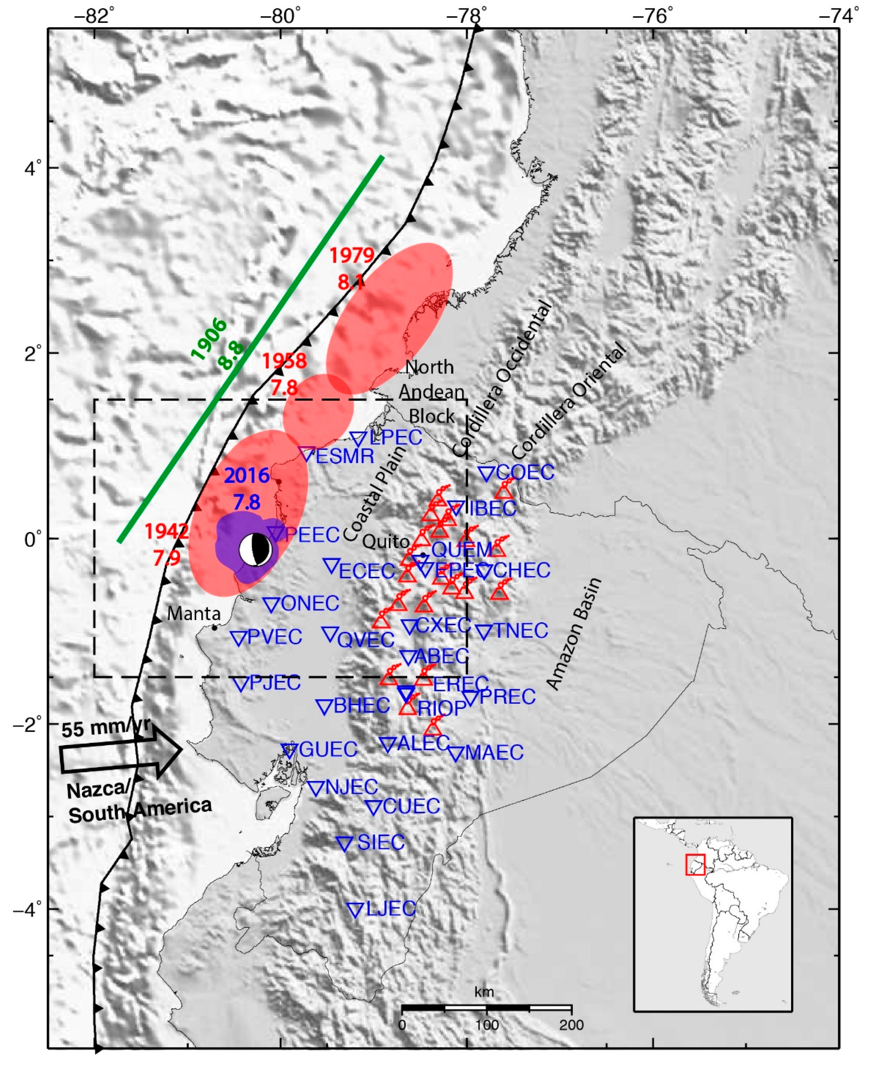
The influence of an earthquake in nearby faults and volcanoes can be evaluated through different methods (see for example [19] and references therein). The Coulomb failure stress criterion is one of the most common analyses used to explain fault interactions and seismological observations after earthquakes, such as aftershocks distribution (e.g., [7,8]).

Although these procedures are commonly used today by the academic community, the transfer of these results to the authorities managing the post-earthquake situation is not straightforward and thus its usefulness is reduced in practice. Providing comprehensible maps to the final user is a pending task.

Here we propose a methodology to evaluate the potential influence of an earthquake on nearby faults and volcanoes and create easy-to-understand maps for decision-making support after an earthquake. We apply this methodology to the Mw 7.8, 2016 Ecuador earthquake that occurred on 16 April 2016 at 23:58:36.980 UTC (https://earthquake.usgs.gov/earthquakes/eventpage/us20005j32#origin). Using Sentinel-1 SAR and continuous GPS data, we measure the coseismic ground deformation and estimate the distribution of slip. Then we use this model to calculate changes of stress on the surrounding faults and volcanoes. The results are compared with the seismic and volcanic events that have occurred after the earthquake. We discuss the potential and limitations of the methodology and the lessons learnt from discussion with local authorities (the Geological Survey of Ecuador, INIGEMM).

2. Study Area

The Pedernales earthquake occurred in the Ecuadorian subduction zone, where the Nazca and South American plates converge at 55 mm/yr [20,21]. The earthquake of Mw 7.8 occurred at 20.6 ± 3.2 km depth (Figure 1) and the focal mechanism is consistent with the rupture of the subduction interface between the Nazca and South American plates. The studies published to date reveal that the Pedernales earthquake ruptured a 100–120 km long segment of the subduction interface and consisted of two main asperities [22,23].

The relative movement of the plates produces M > 7.5 earthquakes (Figure 1) such as the Mw 8.8 1906 Ecuador–Colombia earthquake, which ruptured a large region of 500 km of the subduction interface [30], and the sequence of earthquakes that partially ruptured the same area between 1942 and 1979 (Figure 1). The 2016 Pedernales earthquake seems to have ruptured a similar area to the 1942 earthquake [29]. Apart from megathrust earthquakes, the subduction process is responsible for the uplift of the Andean range [31], crustal faults on the upper plate, and Quaternary volcanism [32].

Continental Ecuador is divided into several morphostructural regions from west to east: the Coastal plain, the Cordillera Occidental, the Cordillera Oriental, and the upper Amazon basin. Active tectonics is dominated by large faults [33] that separate different tectonic regimes including the coastal region, where the subduction of the Carnegie Ridge and the oblique subduction control active structures; the North Andean Block, limited by a NNE dextral strike-slip fault system; and the Eastern Andean Frontal fault zone that limits the North Andean block along the Subandean region. These crustal faults are capable of producing earthquakes, such as the 1987 Ms 6.9 earthquake [34].

3. Data and Methods

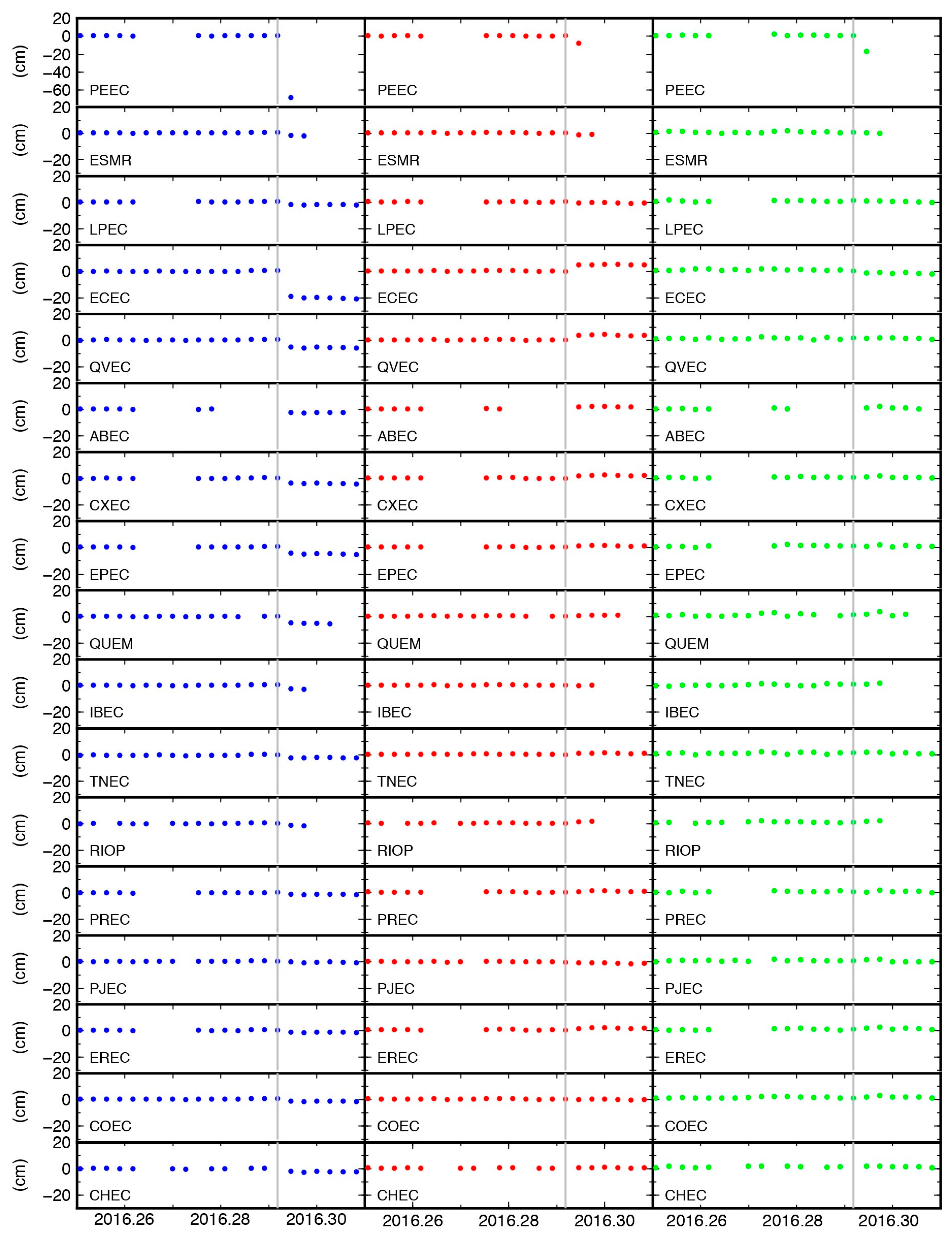
3.1. GPS Displacements

We processed daily RINEX (Receiver Independent Exchange) data from 28 cGNSS stations from the Continuous Monitoring Global Navigation Satellite System (GNSS) Network (REGME) in Ecuador. We estimated the site coordinates before and after the mainshock of the 16 April 2016, Mw7.8 Pedernales Earthquake by using Bernese GPS Software version 5.0 [35], and calculated coseismic displacements by taking the differences between the daily site coordinates. The data were processed on a daily basis using the Bernese Processing Engine (BPE), which applies a double-difference processing strategy. We applied International GNSS Service (IGS) precise orbits and earth orientation parameters, with an absolute antenna phase centre and a FES2004 ocean tide-loading model [36]. Only observations made above an elevation cut-off angle of 5° were used to estimate parameters, and an elevation-dependent weighting was applied. The tropospheric effect was modelled on a prior dry-Niell [37] model and completed by estimating zenith delay corrections for each site at 1-hour intervals using the wet-Niell mapping function. The ambiguity resolution is based on the Quasi-Ionosphere-Free (QIF) baseline-wise analysis. Baselines were constructed based on a strategy of maximum observations.

In order to establish a link with the global reference frame ITRF2008 (IGb08), we use 17 continuously recording GPS stations from the IGS network. Once we obtained the daily solutions and coordinates of REGME stations, we imposed “a posteriori” constraints on implementing the chosen reference frame. The coordinates of the IGS stations were constrained (NNT- No Net Translation option) to their ITRF2008 values.

3.2. InSAR Displacements

We processed Interferometric Synthetic Aperture Radar (InSAR) data from the European Space Agency (ESA) Sentinel-1 satellite to estimate the coseismic line-of-sight (LOS) ground motion. Using the Sentinel-1 processor developed at the Centre Tecnològic de les Telecomunicacions de Catalunya (http://geomatics.cttc.es/remote-sensing/), we combined 2 Sentinel-1 images from descending relative orbit 40, with dates 12 April 2016 and 24 April 2016. The 3-arcsec resolution NASA Shuttle Radar Topographic Mission (SRTM) Digital Elevation Model [38] was used to remove the topographic phase contribution. The interferogram was filtered using a power spectrum filter [39] and unwrapped using the Minimum Cost Flow (MCF) method [40]. The interferogram was geocoded and rectified with a 90 m resolution.

The interferogram was flattened using the GPS displacements as a reference (e.g., [14,41,42]). We first verified that GPS and InSAR data record essentially the same surface displacement, i.e., postseismic deformation in the interferogram is not significant. Although GPS time series covering the same postseismic period included in the interferogram (16–24 April 2016) were not available, we have GPS position time series during a period ranging between 2 and 6 days after the earthquake in most of the GPS network (Supplementary Table S1). In these stations, the difference between GPS coseismic displacements and GPS coseismic displacements plus postseismic displacements is less that 1 cm, which is even smaller when projected in the LOS direction. We can therefore assume that our InSAR and GPS data record essentially the same deformation field. We fitted a linear ramp to the difference between the GPS displacements recorded at the 7 GPS stations that lie inside the region covered by the interferogram (projected onto the local LOS vector) and the InSAR displacements at the same locations. The root mean square (RMS) difference between both datasets is 1.07 cm (Supplementary Table S2).

3.3. Modeling the Earthquake Source (Inversion Method)

We estimate the distribution of slip during the Pedernales earthquake from a linear inversion of the InSAR and GPS displacement field, modelling the earthquake as a dislocation in an elastic medium [43].

We first downsample the InSAR data using a quadtree approach (e.g., [44]) which samples the data according to their spatial variance, leaving more data in regions of high phase gradient near the source. After downsampling, the original ~235,000 data are reduced to ~1000 points. For the inversion, we use the 17 GPS stations closest to the epicentre (Figure 2 and

Table 1. Coseismic displacements at the 17 cGPS sites used in this study.

ID	Location		Displacement (mm)			Error (mm)
	lon	lat	East	North	Up	East	North	Up
ABEC	−78.628	−1.269	−24.46	12.79	7.42	0.27	0.25	0.5
CHEC	−77.814	−0.339	−24.14	2.89	2.59	0.26	0.21	0.61
COEC	−77.787	0.716	−19.60	−3.00	10.31	0.24	0.19	0.5
CXEC	−78.615	−0.935	−41.64	18.51	4.10	0.25	0.2	0.24
ECEC	−79.452	−0.272	−197.32	41.80	−18.83	0.19	0.19	0.57
EPEC	−78.446	−0.315	−50.16	7.21	−3.30	0.27	0.21	0.41
EREC	−78.651	−1.671	−19.07	11.32	15.85	0.21	0.17	0.61
ESMR	−79.724	0.935	−23.50	−13.12	−9.73	0.1	0.09	0.48
IBEC	−78.116	0.350	−29.55	−4.95	2.37	0.19	0.19	0.26
LPEC	−79.164	1.095	−24.60	−7.96	2.99	0.25	0.33	0.41
PEEC	−80.055	0.070	−693.24	−84.13	−175.47	0.22	0.18	0.48
PJEC	−80.425	−1.552	−9.02	−7.34	7.68	0.22	0.23	0.75
PREC	−77.963	−1.708	−10.50	5.25	−8.99	0.23	0.19	0.5
QUEM	−78.497	−0.237	−51.44	4.93	10.40	0.4	0.46	0.47
QVEC	−79.470	−1.012	−56.23	35.24	5.28	0.18	0.18	0.88
RIOP	−78.651	−1.651	−18.39	11.83	10.21	0.13	0.1	0.32
TNEC	−77.816	−0.990	−25.82	8.80	2.09	0.15	0.23	0.32

).

We build the geometry of the subduction interface based on the global subduction zone model of [45] at the latitude of the Pedernales earthquake. We divide it into an array of 450 elements, each measuring 10 km along strike and 10 to 14 km along dip, with a variable dip that increases with depth from 10° to 30°. We jointly invert the InSAR and GPS datasets to solve for the slip distribution along the 450 patches using a least-squares minimization with the non-negativity constraint on the slip. We impose the rake of 123° (from the focal mechanism, http://earthquake.usgs.gov/earthquakes/eventpage/us20005j32#origin). To limit oscillations of the solution, we impose some smoothing on the solution, by minimizing the second-order derivative of the fault slip (e.g., [46]). The linear inversion includes also the weight matrix of each dataset: we tested different weighting to find a compromise between the RMS and the spatial density of the InSAR and GPS dataset. The optimal solution roughness for the final model is selected from the trade-off curve between misfit and solution roughness.

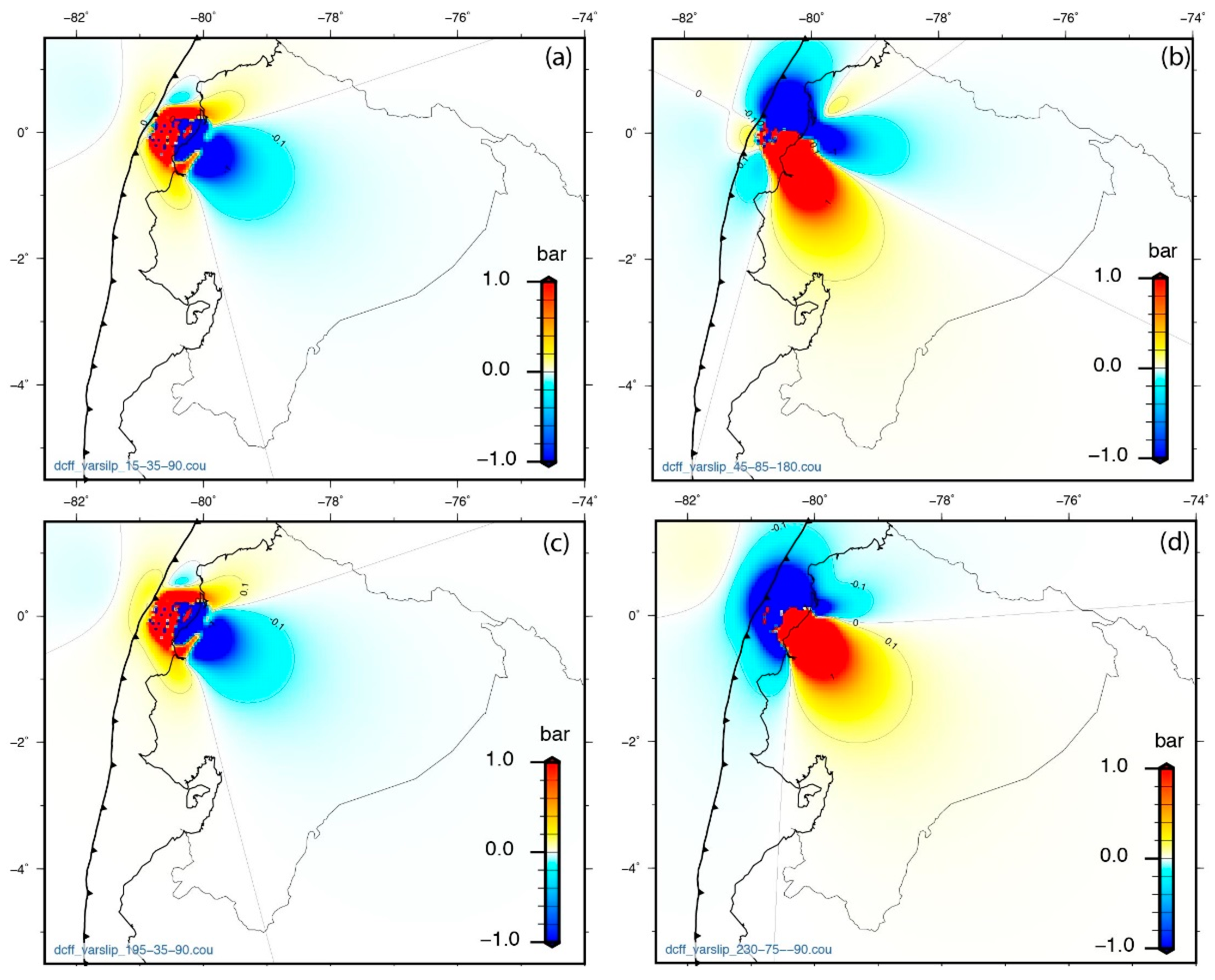
3.4. Estimation of Static Stress Changes

To estimate the static stress changes induced by the Pedernales earthquake we use Coulomb failure stress change ($\Delta CFS$) analysis (e.g., [8,47]). This takes into account the shear and normal stress changes ($\Delta \tau$ and $\Delta \sigma$) induced by the earthquake on selected surfaces or receivers, such as faults or dikes, considering an apparent friction coefficient (${\mu }^{\prime }$) to infer the total coulomb stress, using the equation:

$$\Delta CFS=\Delta \tau -{\mu }^{\prime }\times \Delta \sigma$$

The Coulomb stress change was calculated using Coulomb 3.4 [48], assuming an elastic isotropic half-space characterized by a Shear modulus of 30 GPa and Poisson ratio of 0.25. The apparent (or effective) friction coefficient used for the receiver surfaces is 0.4. Two different source faults are used as input for our Coulomb stress calculations: on the one hand, the variable-slip source model obtained from the joint inversion of InSAR and GPS displacements; on the other hand, the source from the Global CMT focal mechanism with rupture dimensions obtained from [49] empirical relations. The interest of using these two sources is to compare the results using a faster but less well constrained solution (the Global CMT source) with the results obtained using a better-constrained source model from InSAR and GPS data (see Section 5.1). We use the coulomb criteria to estimate the variation of stress induced by the Pedernales earthquake on four different receivers:

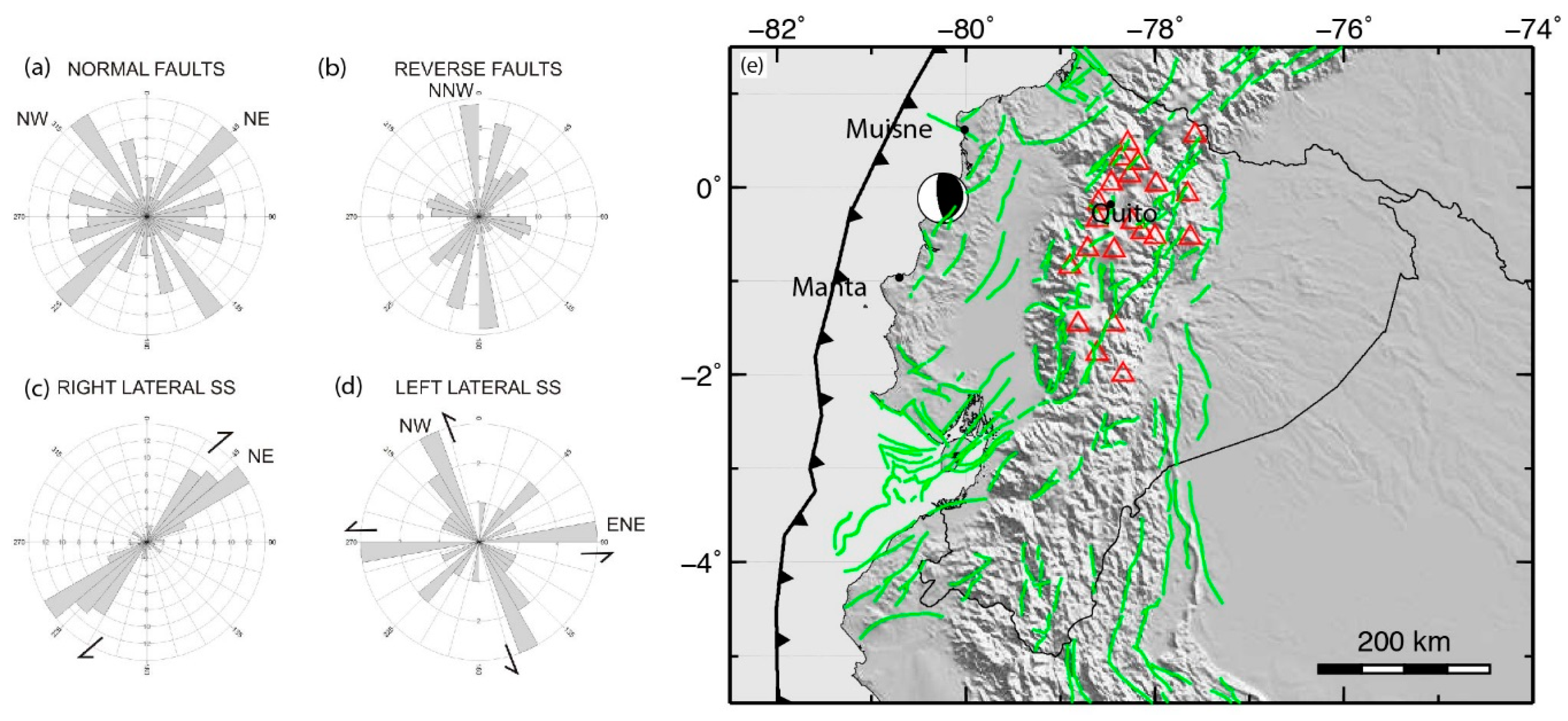
• Potential continental faults: we first select the faults from the catalogue of active faults in Ecuador of [50]. We classify the main sets according to the type of fault: normal, reverse, and strike-slip faults. Additionally, we plot the frequency distribution of fault orientation in rose diagrams. In total, the database shows 278 faults, indicating the fault length, slip direction, plunge of the slip vector, and slip type, among others parameters. For each subset of faults we extract average values of strike, dip, and rake, which are used as receiver fault orientations. We compute stress changes on each fault subset at 10 km depth, which is the common depth for the maximum cortical elastic strength, and therefore the depth for the nucleation of the more relevant earthquakes.
• Known fault traces: from the active faults database of [50] we extracted the fault traces and obtained points spaced 1 km apart along them. Then we estimate the Coulomb failure stress change induced by the Pedernales earthquake on those points with the correspondent potential rupture orientation characteristics (strike, dip, rake), at 5 km depth (the depth of the approximate centre of the modelled fault surfaces).
• Subduction interface: Using the geometry of the subduction interface from [45] we extract the strike, dip, and rake of each node and estimate the Coulomb failure stress change induced by the Pedernales earthquake on each node.
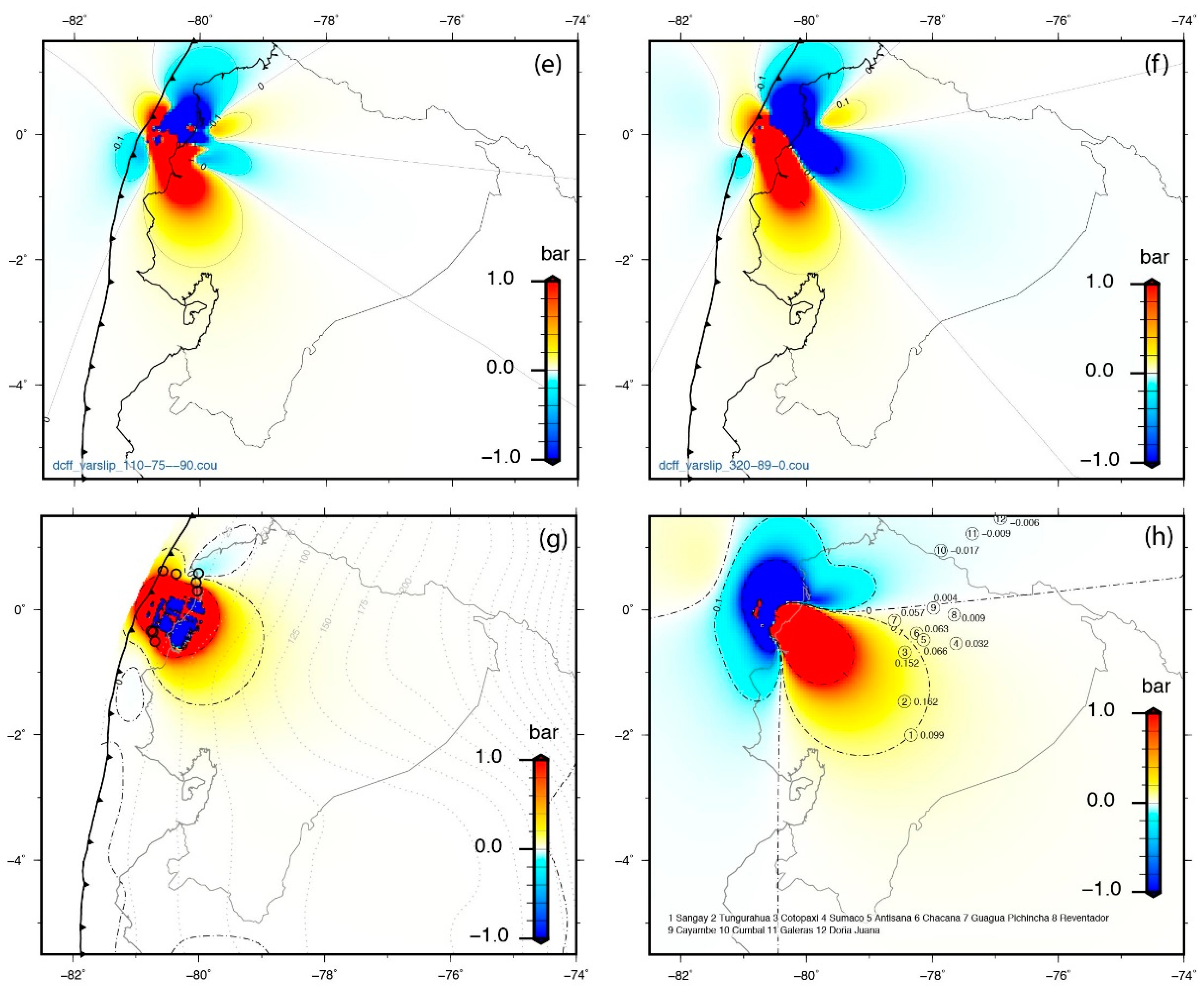
• Volcanoes: we used the Ecuadorian volcanoes with historic activity from The Global Volcanism Program database (http://volcano.si.edu/search_volcano.cfm). We select a set of five currently active volcanoes which have been extensively studied, and extract the orientation of their magma paths, using the criteria of [51] and references therein. We then estimate an average orientation that is used to calculate the induced normal stress change ($\Delta \mathsf{\sigma }$) on the volcano magma pathway. Positive values on a particular volcano indicate unclamping produced by the 2016 earthquake, which indicates dilatation in the crust at the depth of the magma chamber. In this case, the magma pathway is affected by a normal stress reduction or unclamping and this might promote new volcanic eruptions (e.g., [52]). We model the normal stress change at different depths, ranging from 0 to 10 km.

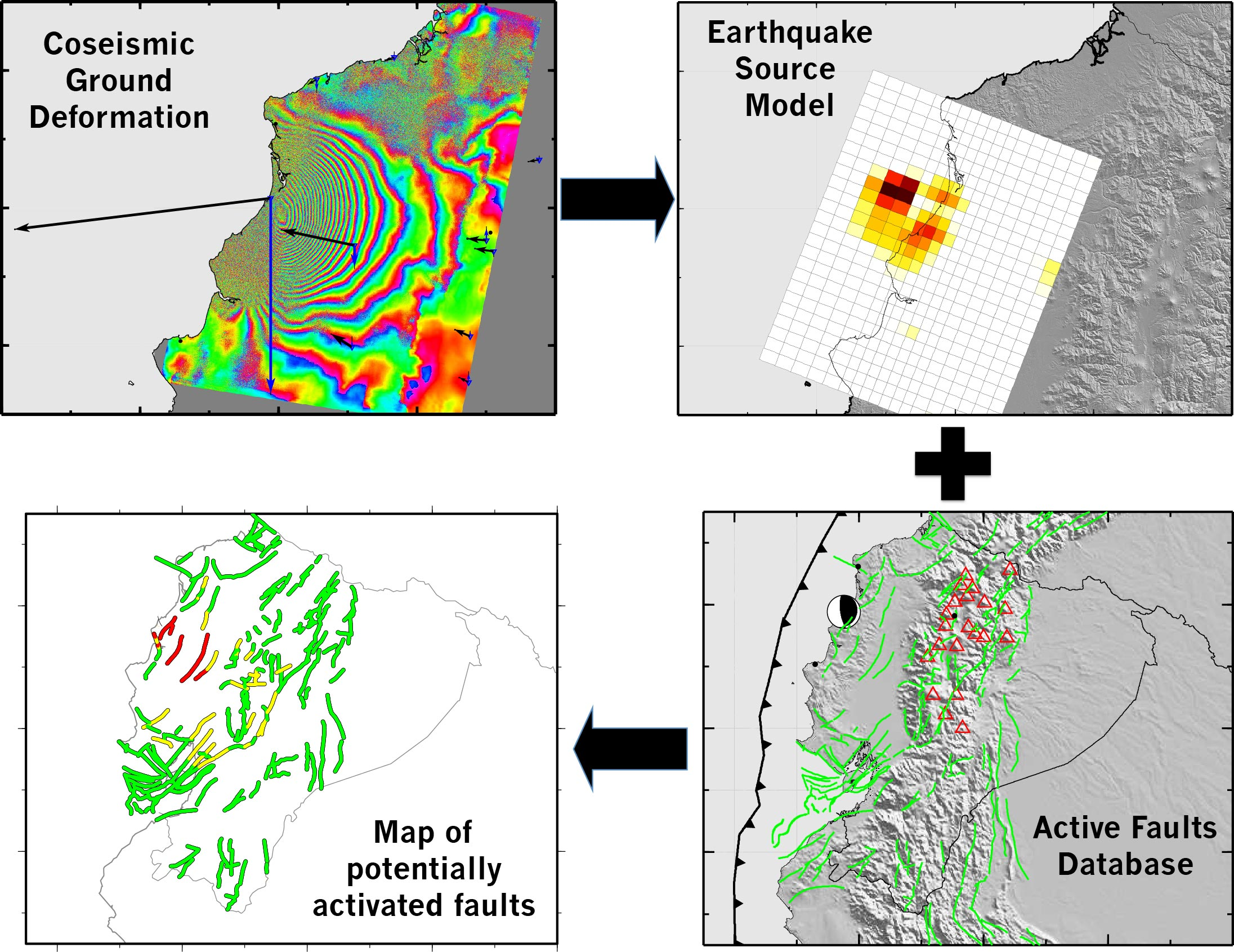
3.5. Final Maps

To produce the final maps we simplify the different maps obtained from the stress change analysis to produce more easy-to-understand maps. We use a traffic light colour coding (red, yellow, green) with three possible values to classify the volcanic and tectonic elements according to their level of potential activation by the Pedernales earthquake. We produce four different maps:

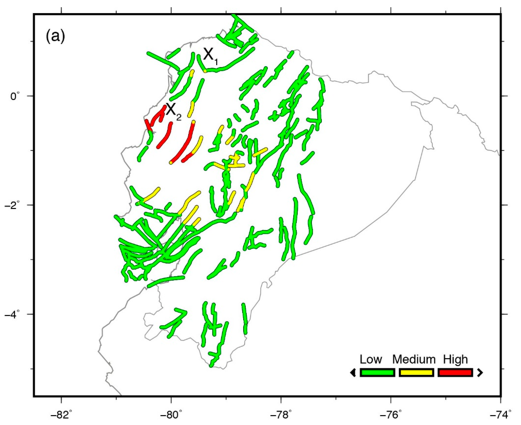
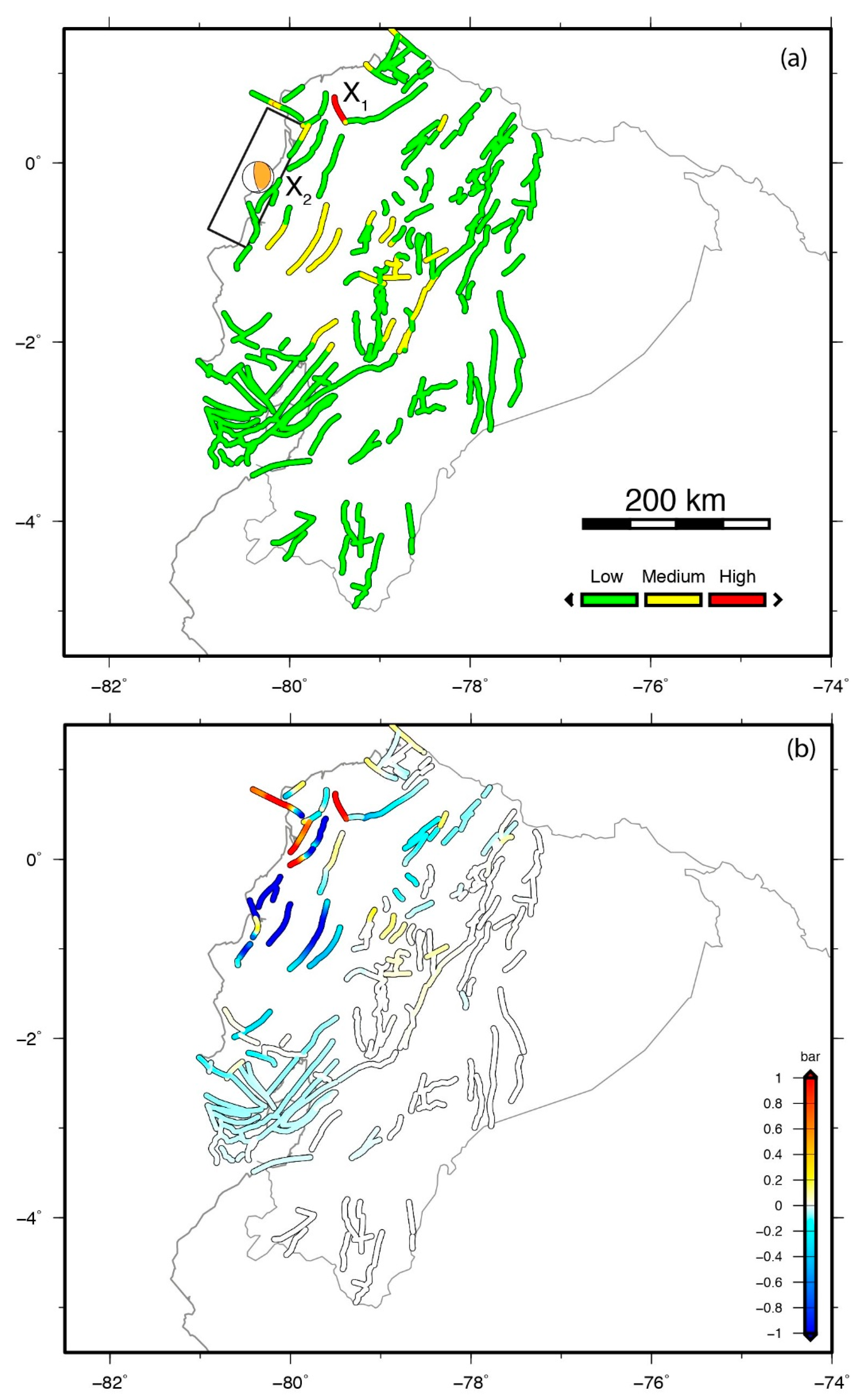
• Map of potentially activated continental faults: We integrate the six different maps of Coulomb stress changes over the correspondent six fault subsets into one map of average positive stress change. We classify the final $\Delta CFS$ values obtained in three levels of potential activation and colour the final map according to those levels: green (low level) indicates areas with $\Delta CFS$ < 0.1 bar, yellow (medium level) indicates areas with 0.1 bar ≤ $\Delta CFS$ ≤ 1 bar, and red (high level) indicates areas with $\Delta CFS$ > 1 bar.
• Map of potentially activated mapped faults: We classify the final $\Delta CFS$ values obtained over each fault trace in three levels of potential activation of the fault segment. Then fault traces are coloured according to those levels: green (low level) indicates faults with $\Delta CFS$ < 0.1 bar, yellow (medium level) indicates fault segments with 0.1 bar ≤ $\Delta CFS$ ≤ 1 bar, and red (high level) indicates faults with $\Delta CFS$ > 1 bar.
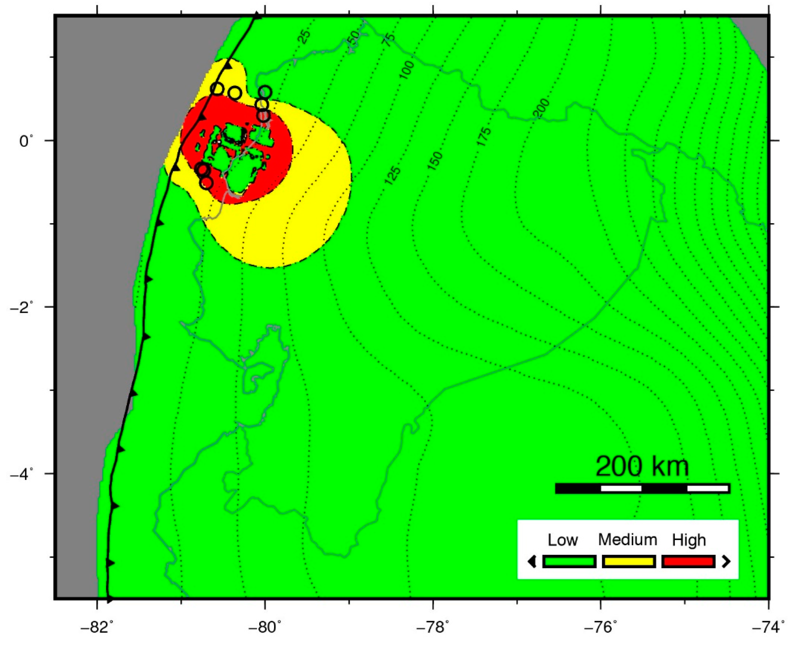
• Map of potentially activated areas on the subduction interface: We classify the final $\Delta CFS$ values obtained over each node of the subduction interface in three levels of potential activation and colour the final map using those levels: green (low level) indicates areas of the slab with $\Delta CFS$ < 0.1 bar, yellow (medium level) indicates areas with 0.1 bar ≤ $\Delta CFS$ ≤ 1 bar, and red (high level) indicates areas with $\Delta CFS$ > 1 bar.
• Map of potentially activated volcanoes: We classify the final $\Delta \mathsf{\sigma }$ values obtained for the average orientation of the volcanoes magma paths in three levels of potential activation and colour the final map according to these levels: green (low level) indicates volcanoes with $\Delta \mathsf{\sigma }$ < 0.01 bar, yellow (medium level) indicates volcanoes with 0.01 bar ≤ $\Delta \mathsf{\sigma }$ ≤ 0.1 bar, and red (high level) indicates volcanoes with $\Delta \mathsf{\sigma }$ > 0.1 bar. The difference in $\Delta \mathsf{\sigma }$ values at depths of 0–10 km is almost identical due to the distance between the Pedernales earthquake source and the volcanic arc (~300 km), and therefore we only represent the value estimated at a depth of 10 km.
• The values used to separate the three intervals of potential seismic or volcanic activation were chosen considering the values published in the literature: in the case of seismic triggering of faults, the lower value of 0.1 bar of $\Delta CFS$ is frequently used as threshold to show areas where aftershocks are triggered (e.g., [53,54,55]), while the higher value (1 bar) is typically related to clear earthquake triggering relations (e.g., [56,57]). In the case of volcanic triggering by unclamping of the magmatic chamber, variations of 0.1 bar have been demonstrated to be influential on the eruptive processes, while the lower value (0.01 bar) is a reasonable threshold to infer a moderate influence from a conservative hazard estimation point of view [58,59,60,61]. Note that a global agreement about the exact values of stress separating triggering from not triggering does not exist and therefore the exact values for our intervals were determined by expert judgment based on our experience and bibliography. These values are subject to modification if the final users consider it appropriate from their experience using those maps.

4. Results

4.1. GPS and InSAR Displacements

The coseismic interferogram (Figure 2) shows a lobe of ground deformation moving away from the satellite, which is located to the left of the image (white arrow labelled LOS in Figure 2). Maximum displacement is ~60 cm of movement away from the satellite. This interferogram covers a period of 12 days (from 12–24 April 2016.), and thus it can also include, apart from deformation associated with the Pedernales mainshock, deformation that occurred during the 8 days after the earthquake.

Position time series of the 17 cGPS sites used in this study are shown in Figure 3. Continuous GNSS data recorded displacements with almost 70 cm of horizontal trenchward motion and subsidence of more than 17 cm near the town of Pedernales (PEEC station, see Figure 2). The sites located near the coast also show subsidence, with areas of uplift found at inland stations (QVEC, ABEC, CXEC, QUEM).

The displacement field observed with both InSAR and GPS data is consistent with onshore ground deformation commonly observed in subduction earthquakes, characterized by subsidence and horizontal trenchward motion (ground experiencing uplift is closer to the trench and often under the ocean, see Supplementary Figure S1).

4.2. Earthquake Source from InSAR and GPS Data

According to our best model, the Pedernales earthquake ruptured a 100-km-long segment of the subduction interface and most of the slip (slip larger than 2 m) occurred between depths of 13 and 30 km (Figure 4). The equivalent geodetic moment of our model is 4.94 × 10²⁰ Nm, considering a shear modulus of 3.3 × 10¹⁰ Pa, and 5.98 × 10²⁰ Nm, considering a shear modulus of 4 × 10¹⁰ Pa, which is consistent with seismological estimates (Mw = 7.8). Slip maxima (asperities) locate in two main areas separated by a lower slip region (<2 m), in agreement with previously published models [28,29,62]. Supplementary Figures S2 and S3 show GPS and InSAR residuals corresponding to this model. The optimal solution roughness for the final model is shown in Supplementary Figure S4.

4.3. Faults and Volcanoes Selected for This Study

The result of the analysis of active faults of Ecuador is shown in Figure 5. The 278 faults of the [50] catalogue can be divided into six families: two sets of normal faults, oriented N45°E and N320°E; two sets of reverse faults, oriented N350°E and N15°E; right-lateral strike slip faults, N60°E trending; and left-lateral strike slip faults that exhibit a conjugate set, N80°E and N330°E (Supplementary Table S3). Furthermore, the total length of each fault type is a relevant parameter to be considered in this analysis. In the case of reverse faulting, fault set with N15°E trending is the 85% of the reverse faulting for fault length larger than 10 km.

The compilation of information on the selected volcanoes (Tungurahua, Guagua Pichincha, Reventardor, Sangay and Cotopaxi) revealed that most of them have vertical or sub-vertical magma paths, with NE-SW azimuths in most of them (see Supplementary Table S4). We use this average orientation to estimate the induced normal stress change ($\Delta \mathsf{\sigma }$) on each volcano magma pathway.

4.4. Results of the Static Stress Analysis

We have produced 8 maps of static stress changes corresponding to the 6 crustal faults families, the subduction interface, the average stress increment taking into account all the fault families and the Ecuadorian volcanoes (Figure 6). We have produced the same set of maps using the Global CMT focal mechanism with rupture dimensions obtained from [49] empirical relations (Supplementary Figure S5).

The results of the stress change analysis on the active faults of Ecuador reveal different patterns of $\Delta CFS$ depending on the orientation of the receiver faults, the receiver fault orientation being one of the most influential parameters on the stress change results. The most extended lobes of $\Delta CFS$ correspond to faults with orientations N45-85, 180 (right hand rule orientation and slip rake), right lateral NE-SW strike slip faults (Figure 6b); and N230-75, -90, NE-SW normal faults (Figure 6d); while smaller lobes correspond to faults N15-35, 90 (Figure 6a) and its conjugate set N195-35, -90 (Figure 6c), NNE-SSW thrust faults. Towards the south of the rupture the families N110-75, -90 (E-W normal faults, Figure 6e) and N320-89, 0 (NW-SE left-lateral strike slip faults, Figure 6f) are stressed. Negative values of $\Delta CFS$ (i.e., inhibition of fault movement) occur mainly offshore and around Muisne.

The results of the stress change analysis on the subduction interface (Figure 6g) show positive values of $\Delta CFS$ downdip and updip of the rupture. Negative values of $\Delta CFS$ are located on areas that slipped during the earthquake.

The results of the stress analysis on the Ecuadorian volcanoes show that the 2016 earthquake increased the normal stress by ≥0.1 bar on 3 of the volcanoes (numbers1, 2, 3 in Figure 6h), with a maximum value of $\Delta \mathsf{\sigma }$ of 0.162 bars at Tungurahua volcano (number 2 in Figure 6h). The volcanoes further north than Cayambe (number 9 in Figure 6h) show negative $\Delta \mathsf{\sigma }$, indicating that the 2016 earthquake induced a normal stress increase on the magma pathway of those volcanoes, which might hinder magmatic activity.

4.5. Final Maps

Following the criteria defined in Section 3.5, we have produced four final maps: potentially activated mapped faults (Figure 7a), potentially activated continental faults (Figure 7b), potentially activated areas on the subduction interface (Figure 8), and potentially activated volcanoes (Figure 9).

The map of potentially activated mapped faults shows that faults with a high level of potential activation (red segments in Figure 7a) are located in the Coastal Plain (region of Manabi) between latitudes −1.5 and 0°N. These faults present values of $\Delta CFS$ > 1 bar induced by the Pedernales earthquake.

The map of potentially activated continental faults shows a main lobe of Coulomb Stress increment towards the southeast of the Pedernales rupture (Figure 7b), and a minor lobe towards the northeast, the later caused mainly by the stress increment on NNE-SSW thrust faulting.

The map of potentially activated areas on the subduction interface shows areas of the slab with a high level of potential activation (red areas in Figure 8) located around the patches of coseismic slip. The regions of the slab with a low level of potential activation (green areas in Figure 8) are found both on areas of coseismic slip and also away from the rupture.

The map of potentially activated volcanoes shows that volcanoes with a high level of potential activation (volcanoes inside the red area, i.e., numbers 2 and 3 in Figure 9) are located to the southeast of the rupture while volcanoes with a low level of potential activation (volcanoes inside the green area, i.e., numbers 8–12 in Figure 9) are those located further north than latitude −0.17°N.

These maps should be interpreted in terms of increased level of potential activation considering only the static stress changes produced by the Pedernales mainshock, but the occurrence of new seismic and volcanic events depends on the state of the system prior to the earthquake. Note that other phenomena not considered in this analysis may also influence the stress state of the crust and trigger or inhibit new seismic and volcanic events (see Section 5.2 and 5.3).

5. Discussion

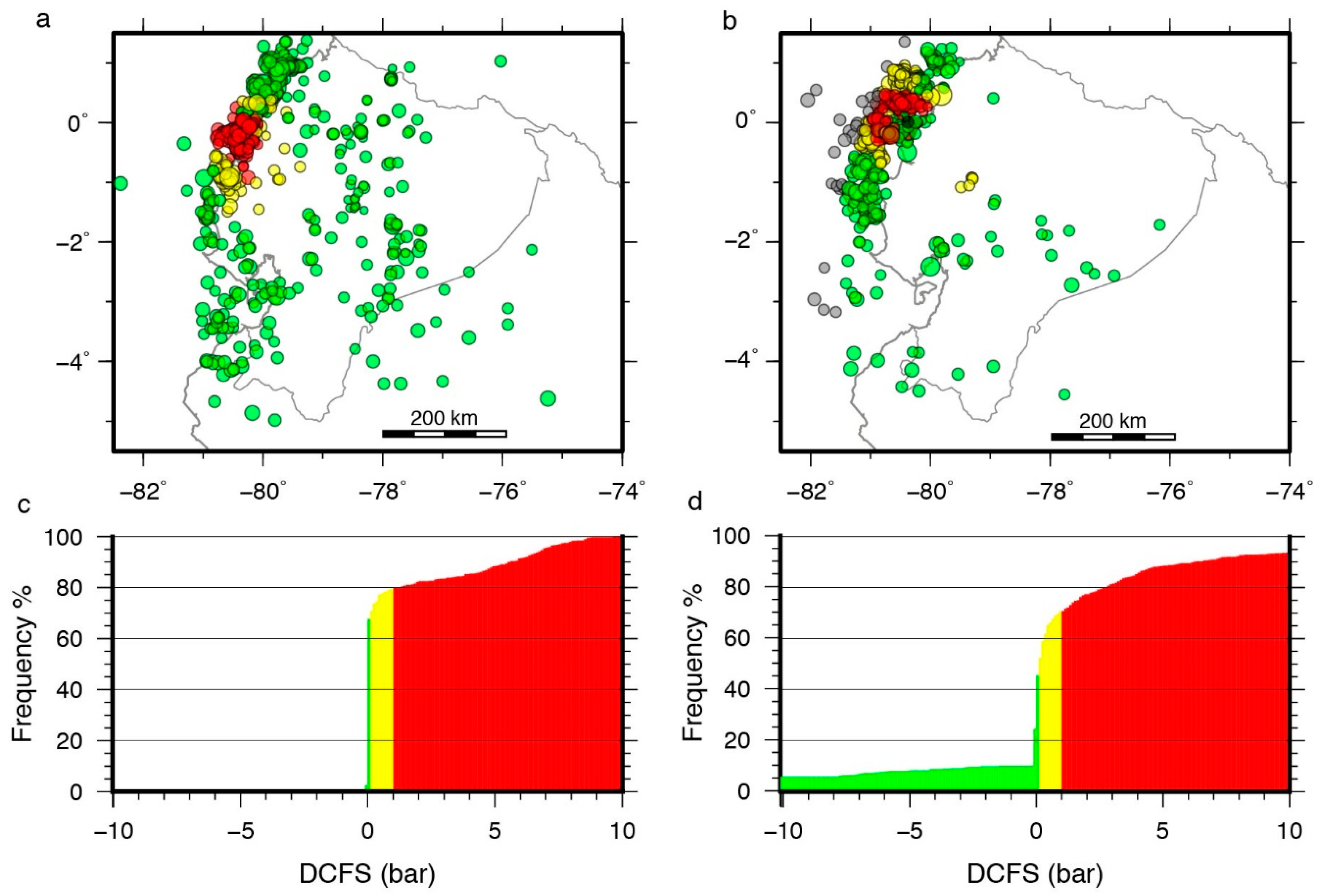
5.1. Models Using the Focal Mechanism

We performed our calculations of static Coulomb failure stress changes associated with the Pedernales earthquake slip using as an alternative source the Global CMT focal mechanism. The interest of using such source is the promptness with which focal mechanisms are available (even a few minutes after the earthquake) compared to the source derived from InSAR and GPS data (days to weeks). Figure 10a shows the map of potentially activated mapped faults of Ecuador calculated using the earthquake source from the Global CMT. Compared with the map created using our source (Figure 7), the level of potential activation on mapped faults is lower using the CMT source and fault segments with a high level of potential activation (red segments) are not the same in both maps.

We have computed the difference between both maps to identify their main similarities and differences (Figure 10b). The CMT model produces very similar results in faults far from the earthquake source (white segments in Figure 10b). For closer receivers the variation is, however, significant: for example, the fault labelled X₁ in Figure 7 and Figure 10a shows a low level of potential activation in the map created using our source and a high level of potential activation in the map created using the CMT source. A similar case is the segment labelled X₂ in Figure 7 and Figure 10a, with low values in the CMT map and high values in the map derived from our source. This effect is common on every modelled earthquake, in the near field the details and particularities of the slip distribution is one of the key parameters that define the stress change field [63]; while in the far field the slip details are less relevant and the approximate dimensions of the source and the earthquake magnitude is enough to define a valid stress change field.

Since the static stress change is highly dependent on the slip distribution, the more data we can add for the inversion of the source, the more reliable will be our final model. Using the focal mechanism to produce a preliminary version of the maps can allow fast results after the earthquake, but they should be updated using a better constrained source model when new observations, particularly from seismological and geodetic networks that accurately observe the earthquake process, are available.

5.2. Comparison of Our Final Maps with Seismic and Volcanic Events

We have compared seismic events with magnitudes between 2 and 6.9 in the period 16 April 2016–18 February 2018 with our final maps. Using the seismic events from Instituto Geofísico Escuela Politécnica Nacional we have separated events that occurred in the subduction interface (selecting events at a distance ≤10 km from the slab) from events that occurred in continental faults (selecting events with distance to slab >10 km and depth <15 km). Figure 11a,b show the events that occurred in continental faults and in the subduction interface, respectively, coloured according to the traffic light colour coding in Figure 7b and Figure 8. Red circles represent seismic events located in areas with a high level of potential activation (∆CFS > 1 bar), yellow circles represent seismic events in areas with a medium level of potential activation (0.1 bar ≤ ∆CFS ≤ 1), and green circles represent seismic events in areas with a low level of potential activation (∆CFS < 0.1 bar). We have quantified the number of events located on each region (histograms in Figure 11 c,d) for events that occurred on the subduction interface (Figure 11d), 50% of the events occurred in areas with a high or medium level of potential activation. For events that occurred at continental faults (Figure 11c), only 35% of events occurred in areas with a high or medium level of potential activation. This can be explained by different factors: on the one hand, the seismic events analysed are not relocated, and thus the final location of the events can vary from the one shown in Figure 11a,b. Moreover, our models only consider static stress changes induced by the Pedernales earthquake, but other significant seismic events have occurred in the period April 2016–February 2018 that have also changed the stress state of the crust. For instance, the three largest events that have occurred after the Pedernales earthquake (Supplementary Figure S8) with Mw 6.3, 6.7, and 6.9, located near Muisne, to the north of the main shock rupture, may have triggered many of the seismic events located in that area in Figure 11a,b. Additionally, other processes apart from static stress changes, such as dynamic stresses or postseismic phenomena, may influence the stress of the crust. This will be discussed in Section 5.3.

If we only consider the largest events that occurred in the region after the Pedernales earthquake (Mw ≥ 6, Supplementary Figure S8) during the same period, the correlation with our maps is clearer. Since the location and focal mechanism of these events is consistent with the subduction interface between the Nazca and the South American plates, we have compared their location with the map of Coulomb failure stress change on the subduction interface (black circles in Figure 6g). Most of the aftershocks nucleated in areas of increased ∆CFS surrounding the mainshock slip patches. Overall, more than 87% of the Mw ≥ 6 aftershocks (7 of 8 events) occurred in areas of ∆CFS > 0.1 bar. We also compared the location of these events with the map of potentially activated areas on subduction interface (black circles in Figure 8). Fifty percent of the events occurred in areas with a high level of potential activation, 37.5% of the events occurred in areas with a medium level of potential activation, and 12.5% of the events occurred in areas with a low level of potential activation. Our map is therefore useful to constrain the areas where the largest aftershocks will nucleate after the mainshock.

Regarding volcanic activity in Ecuador, according to Instituto Geofisico (http://www.igepn.edu.ec/informes-volcanicos) at least two volcanoes in the Galapagos Islands have shown volcanic activity or periods of unrest after the Pedernales earthquake: the Fernandina volcano, in eruption since September 2017, and the Sierra Negra volcano, that shows seismic activity since July 2017 and an uplift rate of 70 cm/yr (http://www.igepn.edu.ec/servicios/noticias/1539-informe-especial-sierra-negra-n-2-2017). However, Galápagos Islands are more than 1000 km away from the Pedernales earthquake source and thus the static stress changes induced by the Pedernales earthquake on these volcanoes are too small to trigger volcanic activity, although dynamic stresses associated to the elastic waves propagation could be responsible. In continental Ecuador, two volcanoes present a high level of potential activation (Cotopaxi and Tungurahua) and Sangay volcano is very close to the boundary of the high level too (Figure 9). Using data from https://volcano.si.edu/volcano.cfm?vn=352090 and https://www.volcanodiscovery.com, information about the volcanic activity of these volcanoes during the month after the earthquake (including ash emission, presence of thermal anomalies, and significant seismic activity) was collected.

• Sangay volcano awoke one month before the earthquake (26 April 2016), according to reports about ash emission and thermal anomaly. Ash emission was ongoing during at least two months, and the thermal anomaly was recorded in the same period (12 May 2016). After that, both ash emissions and thermal anomalies were intermittent through July 2016.
• In the vicinity of Cotopaxi volcano, two earthquakes of magnitude 3 and 3.1 occurred at a distance of 15 km from the volcano on 17 April 2016, the day after the Pedernales earthquake.
• Near Tungurahua volcano, five earthquakes were recorded between 17 April 2016 and 19 May 2016, with magnitudes ranging between 2.8 and 3.2 and distances between 21 to 33 km away from the volcano.

Therefore, significant volcanic activity seems to have increased in these volcanoes around the date of the earthquake, suggesting a potential relationship between both phenomena.

5.3. Potential and Limits of the Methodology

Nowadays several SAR satellites such as Sentinel-1A/B, ALOS-2, CSK, TSK, allow the production of coseismic interferogramas relatively quickly (from hours to a few days) after an earthquake. The new European Space Agency (ESA) Sentinel-1 constellation is particularly well adapted to this task, since it acquires images globally every 6–12 days, that are distributed free of charge. In the coming years, several initiatives now in the testing phase to produce systematic interferograms should be fully operational (e.g., GEP, LicS, ARIA, EPOS).

Coseismic GPS displacements are not globally available and their accessibility depends on different factors, including the previous existence of a permanent and non-permanent GPS networks in the zone. Although more and more countries have a continuous GPS network, the data are rarely public. However, some international initiatives exist to give access to GPS data, such as UNAVCO consortium (http://www.unavco.org/) that provides Open Access GPS data with daily RINEX files suitable for processing, although they mostly cover the United States and Caribbean zones. Similarly, the European Plate Observing System will soon provide access to GNSS data in real time over Europe (https://www.epos-ip.org/tcs/gnss-data-and-products). The availability of real-time High-Rate Global Positioning System (HRGPS) data can be used to produce rapid magnitude estimation and produce rapid earthquake source models (e.g., [64]).

Finite source models from InSAR and GNSS data can be performed using open-source software tools such as RELAX (https://geodynamics.org/cig/software/relax/), Pyrocko (https://pyrocko.org/), and Defnode (http://www.web.pdx.edu/~mccaf/defnode.html). Including other data in the inversion, such as seismological or tsunami data, can be helpful to constrain the offshore part of the source model (e.g., [29]). Our methodology can also be applied using other earthquake sources, such as focal mechanisms or finite fault models from Global Seismic Network (GSN) broadband waveforms (e.g., https://earthquake.usgs.gov/earthquakes/eventpage/us20005j32#finite-fault), that are publicly available after earthquakes.

One of the more time consuming steps when applying this methodology is the compilation of faults and volcanic elements to build the models. In the case of subduction earthquakes, the global model for subduction geometries of [45] can be downloaded from (https://earthquake.usgs.gov/data/slab/). Crustal faults are more difficult to obtain, and despite the important efforts towards the systematization and compilation of active sources (GEM, Global Active Faults: https://github.com/GEMScienceTools/gem-global-active-faults; SHARE, European Database of Seismogenic Faults: http://diss.rm.ingv.it/share-edsf/SHARE_WP3.2_Database.html) the completeness of the catalogue or the level of detail and the parameterization of the fault elements usually requires further analysis. The existence of national publicly available databases (e.g., the Quaternary Active Faults Database of Iberia, http://info.igme.es/qafi/, the New Zealand Active Faults Database http://data.gns.cri.nz/af/, the database of active faults in Greece [65]) is a great advantage in these cases. However, the main factor that determines the quality of the resulting maps is the quality, reliability, and completeness of the database (i.e., how reliable the faults and volcanoes parameters are). For instance, unmapped faults can result in unexpected triggered earthquakes, such as the case of the Christchurch earthquake [66]. The reliability of the maps will increase as the knowledge and characterization of active faults and volcanic system improves.

The static Coulomb stress criterion, although a simplistic approach, is a powerful tool to explain many fault and volcanic interactions and is issued as a tool for earthquake forecasting (e.g., [7,19,67]). Different scientific software can be used to carry out these models (e.g., Coulomb 3.3 [48], RELAX [68]).

Apart from the fault–fault or fault–volcano interactions analysed in this study, other interactions can occur that could be taken into account, for example, aftershocks and postseismic deformation (e.g., [14]), volcanic interactions (e.g., [69]), or coseismic-induced landslides (e.g., [70]). Beyond the static stress changes estimated here, other mechanisms such dynamic stresses, pore-fluid diffusion, and viscoelastic rebound can also be important for different time frames after the earthquake. Additionally, the incorporation of relevant aftershocks into the models, as well as postseismic phenomena, can improve the hazard estimation and focus these tools towards an operational forecasting system.

Finally, a close collaboration with the final user is critical to create functional and useful products. The comprehension of our final maps was significantly improved thanks to the constructive criticisms and specific proposals of the Geological Survey of Ecuador staff (Instituto Nacional de Investigación Geológico Minero Metalúrgico, INIGEMM).

6. Conclusions

We present a methodology to evaluate earthquake-induced effects on neighbouring faults and volcanoes and create easily understandable maps addressed to decision-makers managing the post-earthquake situation. The first part of the method involves estimating the earthquake source model from space geodetic data, the second part consists in using this model as input to calculate static stress changes on tectonic and volcanic elements in the vicinity of the earthquake, and the third part is the creation of the final maps by synthetizing and simplifying the results for non-experts.

We apply the methodology to the Mw 7.8, 2016 Pedernales earthquake, Ecuador. Using Sentinel-1 InSAR and GPS data, we estimate the coseismic deformation field associated with the Pedernales earthquake and invert this field to model the source. Then, we calculate static stress changes on the subduction interface, on the active continental faults of Ecuador and on the volcanoes. The resulting maps show areas of high, medium, and low levels of potential activation of faults or volcanoes. When compared with seismic and volcanic event occurred after the Pedernales earthquake, we found in general a good agreement, with most of the largest aftershocks nucleated in areas of stress loading in our maps. Seismic and volcanic events located in areas of low level of potential activation in our maps are probably due to other phenomena not considered in our analysis, such as static stress changes from large aftershocks, dynamic stresses, or postseismic phenomena.

Our maps are useful to identify regions where new volcanic or seismic events are more likely to happen taking into account the static stress changes produced by the mainshock. But our models do not take into account the influence of other processes, such as dynamic stress changes produced by the earthquake, postseismic phenomena, or other tectonic and volcanic activity of the region. Hence, other seismic or volcanic events could occur out of the critical areas depicted in the proposed maps (red and yellow colours).

One of the main limitations of the methodology is the static stress approach, since other earthquake-related processes can also influence the behaviour of faults and volcanoes (dynamic stresses, pore-fluid diffusion, viscoelastic rebound). Also, an important limitation is the time necessary to have a new SAR acquisition over the earthquake area, which usually takes several days. This could be overcome using in the meantime the focal mechanism as a first-order earthquake source.

Considering the open data policy of Sentinel-1 SAR data, the availability of tools for the estimation of the earthquake source, and the evaluation of static stress changes, the methodology proposed here can be applied to earthquakes worldwide to quickly generate these maps after the earthquake and update them when additional data (e.g., GPS data, coseismic interferograms from other satellites, seismological and tsunami data) are available.

References

1. Freed, A.M. Earthquake triggering by static, dynamic, and postseismic stress transfer. Annu. Rev. Earth Planet. Sci. 2005, 33, 335–367. [Google Scholar] [CrossRef]
2. King, G.C.P.; Deves, M. Fault interaction, earthquake stress changes, and the evolution of seismicity. In Treatise of Geophysics, 2nd ed.; Elsevier: Amsterdam, The Netherlands, 2015; Volume 4, pp. 243–269. [Google Scholar]
3. Scholz, C.H. The Mechanics of Earthquakes and Faulting; Cambridge University Press: New York, NY, USA, 2002; p. 471. [Google Scholar]
4. Toda, S.; Stein, R.S.; Reasonberg, P.A.; Dieterich, J.H.; Yoshida, A. Stress transferred by the 1995 Mw = 6.9 Kobe, Japan, shock: Effect on aftershocks and future earthquake probabilities. J. Geophys. Res. 1995, 103, 24543–24565. [Google Scholar] [CrossRef]
5. Parsons, T.; Stein, R.S.; Simpson, R.W.; Reasenberg, P.A. Stress sensitivity of fault seismicity: A comparison between limited-offset oblique and major strike-slip faults. J. Geophys. Res. 1999, 104, 20183–20202. [Google Scholar] [CrossRef] [Green Version]
6. Kilb, D.; Gomberg, J.; Bodin, P. Aftershock triggering by complete Coulomb stress changes. J. Geophys. Res. 2002. [Google Scholar] [CrossRef]
7. Lin, J.; Stein, R.S. Stress interaction in thrust and subduction earthquakes. J. Geophys. Res. 2004. [Google Scholar] [CrossRef]
8. King, G.C.P.; Stein, R.S.; Lin, J. Static stress changes and the triggering of earthquakes. Bull. Seismol. Soc. Am. 1994, 84, 935–953. [Google Scholar]
9. Lettis, W.; Bachhuber, J.; Witter, R.; Brankman, C.; Randolph, C.E.; Barka, A.; Page, W.D.; Kaya, A. Influence of releasing step-overs on surface fault rupture and fault segmentation: Examples from the 17 August 1999 Izmit earthquake on the North Anatolian fault, Turkey. Bull. Seismol. Soc. Am. 2002, 92, 19–42. [Google Scholar] [CrossRef]
10. Hill, D.P.; Reasenberg, P.A.; Michael, A.J.; Arabasz, W.J.; Beroza, G.C. Seismicity remotely triggered by the magnitude 7.3 Landers, California earthquake. Science 1993, 260, 1617–1623. [Google Scholar] [CrossRef] [PubMed]
11. Anderson, J.G.; Brune, J.N.; Louie, J.N.; Zeng, Y.H.; Savage, M.; Yu, G.; Chen, Q.; de Polo, D. Seismicity in the western Great Basin apparently triggered by the Landers, California, earthquake 28 June 1992. Bull. Seismol. Soc. Am. 1994, 84, 863–891. [Google Scholar]
12. Hill, D.P.; Pollitz, F.; Newhall, C. Earthquake-volcano interactions. Phys. Today 2002, 55, 41–47. [Google Scholar] [CrossRef]
13. Walter, T.R.; Amelung, F. Volcanic eruptions following M ≥ 9 megathrust earthquakes: Implications for the Sumatra-Andaman volcanoes. Geology 2007, 35, 539–542. [Google Scholar] [CrossRef]
14. Béjar-Pizarro, M.; Carrizo, D.; Socquet, A.; Armijo, R.; Barrientos, S.; Bondoux, F.; Bonvalot, S.; Campos, J.; Comte, D.; de Chabalier, J.B.; et al. Vigny Asperities, barriers and transition zone in the North Chile seismic gap: State of the art after the 2007 Mw 7.7 Tocopilla earthquake inferred by GPS and InSAR data. Geophys. J. Int. 2010, 183, 390–406. [Google Scholar] [CrossRef] [Green Version]
15. Vigny, C.; Socquet, A.; Peyrat, S.; Ruegg, J.C.; Métois, M.; Madariaga, R.; Morvan, S.; Lacassin, R.; Campos, J.; Carrizo, D.; et al. The 2010 Mw 8.8 Maule Megathrust Earthquake of Central Chile, Monitored by GPS. Science 2011, 332, 1417–1421. [Google Scholar] [CrossRef] [PubMed]
16. Elliott, J.R.; Walters, R.J.; Wright, T.J. The role of space-based observation in understanding and responding to active tectonics and earthquakes. Nat. Commun. 2016, 7, 13844. [Google Scholar] [CrossRef] [PubMed] [Green Version]
17. Hamling, I.J.; Hreinsdóttir, S.; Clark, K.; Elliott, J.; Liang, C.; Fielding, E.; Litchfield, N.; Villamor, P.; Wallace, L.; Wright, T.J.; et al. Complex multifault rupture during the 2016 M 7.8 Kaikoura earthquake. New Zealand. Science 2017, 356, eaam7194. [Google Scholar] [CrossRef] [PubMed]
18. Jones, B.K.; Stryker, T.S.; Mahmood, A.; Platzeck, G.R. The International Charter ‘Space and Major Disasters’. In Time-Sensitive Remote Sensing; Lippitt, C.D., Stow, D., Coulter, L., Eds.; Springer: New York, NY, USA, 2015; pp. 79–89. [Google Scholar]
19. Harris, R.A. Introduction to special section: Stress triggers, stress shadows, and implications for seismic hazard. J. Geophys. Res. 1998, 103, 347–358. [Google Scholar] [CrossRef]
20. Kendrick, E.; Bevis, M.; Smalley, J.R.; Brooks, B.; Vargas, R.B.; Lauria, E.; Souto Fortes, L.P. The Nazca–South America Euler vector and its rate of change. J. S. Am. Earth Sci. 2003, 16, 125–131. [Google Scholar] [CrossRef]
21. Nocquet, J.M.; Villegas-Lanza, J.C.; Chlieh, M.; Mothes, P.A.; Rolandone, F.; Jarrin, P.; Cisneros, D.; Alvarado, A.; Audin, L.; Bondoux, F.; et al. Motion of continental slivers and creeping subduction in the northern Andes. Nat. Geosci. 2014, 7, 287–291. [Google Scholar] [CrossRef]
22. Nocquet, J.M.; Jarrin, P.; Vallée, M.; Mothes, P.A.; Grandin, R.; Rolandone, F.; Delouis, B.; Yepes, H.; Font, Y.; Fuentes, D.; et al. Supercycle at the Ecuadorian subduction zone revealed after the 2016 Pedernales earthquake. Nat. Geosci. 2017, 10, 145–149. [Google Scholar] [CrossRef]
23. Ye, L.; Kanamori, H.; Avouac, J.P.; Li, L.; Cheung, K.F.; Lay, T. The 16 April 2016, MW 7.8 (MS 7.5) Ecuador earthquake: A quasi-repeat of the 1942 MS 7.5 earthquake and partial re-rupture of the 1906 MS 8.6 Colombia–Ecuador earthquake. Sci. Lett. 2016, 454, 248–258. [Google Scholar] [CrossRef]
24. Amante, C.; Eakins, B.W. ETOPO1 1 Arc-Minute Global Relief Model: Procedures, Data Sources and Analysis; NOAA Technical Memorandum NESDIS NGDC-24; National Geophysical Data Center-NOAA: Boulder, CO, USA, 2009.
25. Kelleher, J. Rupture zones of large South American earthquakes and some predictions. J. Geophys. Res. 1972, 77, 2087–2103. [Google Scholar] [CrossRef]
26. Kanamori, H.; McNally, K.C. Variable rupture mode of the subduction zone along the Ecuador–Colombia coast. Bull. Seismol. Soc. Am. 1982, 72, 1241–1253. [Google Scholar]
27. Mendoza, C.; Dewey, J.W. Seismicity associated with the great Colombia—Ecuador earthquakes of 1942, 1958 and 1979: Implications for barrier models of earthquake rupture. Bull. Seismol. Soc. Am. 1984, 74, 577–593. [Google Scholar]
28. Bilek, S.L. Seismicity along the South American subduction zone: Review of large earthquakes, tsunamis, and subduction zone complexity. Tectonophysics 2010, 495, 2–14. [Google Scholar] [CrossRef]
29. Chlieh, M.; Mothes, P.A.; Nocquet, J.M.; Jarrin, P.; Charvis, P.; Cisneros, D.; Font, Y.; Collot, J.Y.; Villegas-Lanza, J.C.; Rolandone, F.; et al. Distribution of discrete seismic asperities and aseismic slip along the Ecuadorian Megathrust. Earth Planet. Sci. Lett. 2014, 400, 292–301. [Google Scholar] [CrossRef]
30. Álvarez-Gómez, J.A.; Aniel-Quiroga, Í.; Gutiérrez-Gutiérrez, O.Q.; Larreynaga, J.; González, M.; Castro, M.; Gavidia, F.; Aguirre-Ayerbe, I.; González-Riancho, P.; Carreño, E.; et al. Tsunami hazard assessment in El Salvador, Central America, from seismic sources through flooding numerical models. Nat. Hazards Earth Syst. Sci. 2013, 13, 2927–2939. [Google Scholar] [CrossRef] [Green Version]
31. Jordán, T.E.; Isacks, B.L.; Allmendinger, R.W.; Brewer, J.A.; Ramos, V.A.; Ando, C.J. Andean tectonics related to geometry of subducted Nazca plate. Geol. Soc. Am. Bull. 1983, 94, 341–361. [Google Scholar] [CrossRef]
32. Hall, M.L.; Wood, C.A. Volcano-tectonic segmentation of the northern Andes. Geology 1985, 13, 203–207. [Google Scholar] [CrossRef]
33. Eguez, A.; Alvarado, A.; Yepes, H.; Machette, M.N.; Costa, C.; Dart, R.L. Database and Map of Quaternary Faults and Folds of Ecuador and Its Offshore Regions; USGS Open-File Report 03-289; USGS: Reston, VA, USA, 2003.
34. National Research Council of National Academy Sciences (NRC-NAS). The March 5, 1987 Ecuador Earthquakes: Mass Wasting and Socioeconomic Effects; National Research Council of National Academy Sciences Studies in Natural Disasters; The National Academies Press: Washington, DC, USA, 1991; Volume 5, p. 163.
35. Dach, R.; Hugentobler, U.; Fridez, P. Meindl, M. Bernese GPS Software Version 5.0. Astronomical Institute; University of Berne: Bern, Switzerland, 2007. [Google Scholar]
36. Lyard, F.; Lefevre, F.; Letellier, T.; Francis, O. Modelling the global ocean tides: Modern insights from FES2004. Ocean Dyn. 2006, 56, 394–415. [Google Scholar] [CrossRef]
37. Niell, A.E. Global mapping functions for the atmosphere delay at radio wavelengths. J. Geophys. Res. Solid Earth 1996, 101, 3227–3246. [Google Scholar] [CrossRef]
38. Farr, T.G.; Kobrick, M. Shuttle radar topography mission produces a wealth of data. Eos Trans. Am. Geophys. Union 2000, 81, 583–585. [Google Scholar] [CrossRef]
39. Goldstein, R.M.; Werner, C.L. Radar interferogram filtering for geophysical applications. Geophys. Res. Lett. 1998, 25, 4035–4038. [Google Scholar] [CrossRef] [Green Version]
40. Costantini, M. A novel phase unwrapping method based on network programming. IEEE Trans. Geosci. Remote Sens. 1998, 36, 813–821. [Google Scholar] [CrossRef]
41. Pritchard, M.E.; Norabuena, E.O.; Jillings, C.; Boroschek, R.; Comte, D.; Simons, M.; Dixon, T.H.; Rosen, P.A. Geodetic, teleseismic, and strong motion constraints on slip from recent southern Peru subduction zone earthquakes. J. Geophys. Res. 2007, 112, B03307. [Google Scholar] [CrossRef]
42. Grandin, R.; Klein, E.; Métois, M.; Vigny, C. Three-dimensional displacement field of the 2015 Mw8.3 Illapel earthquake (Chile) from across- and along-track Sentinel-1 TOPS interferometry. Geophys. Res. Lett. 2016, 43. [Google Scholar] [CrossRef]
43. Okada, Y. Surface deformation to shear and tensile faults in a half space. Bull. Seismol. Soc. Am. 1985, 75, 1135–1154. [Google Scholar]
44. Jonsson, S.; Zebker, H.; Segall, P.; Amelung, F. Fault slip distribution of the 1999 Mw 7.1 Hector Mine, California, earthquake, estimated from satellite radar and GPS measurements. Bull. Seismol. Soc. Am. 2002, 92, 1377–1389. [Google Scholar] [CrossRef]
45. Hayes, G.P.; Wald, D.J.; Johnson, R.L. Slab1.0: A three-dimensional model of global subduction zone geometries. J. Geophys. Res. 2012, 117, B01302. [Google Scholar] [CrossRef]
46. Harris, R.A.; Segall, P. Detection of a locked zone at depth on the Parkfield, California, segment of the San Andreas fault. J. Geophys. Res. 1987, 92, 7945–7962. [Google Scholar] [CrossRef]
47. Stein, R.S.; King, G.C.P.; Lin, J. Change in failure stress on the southern San Andreas fault system caused by the 1992 magnitude = 7.4 Landers earthquake. Science 1992, 258, 1328–1332. [Google Scholar] [CrossRef] [PubMed]
48. Toda, S.; Stein, R.S.; Sevilgen, V.; Lin, J. Coulomb 3.3: Graphic-Rich Deformation and Stress-Change Software for Earthquake, Tectonic, and Volcano Research and Teaching—User Guide: U.S. Geological Survey Open-File Report 2011–1060; USGS: Reston, VA, USA, 2011.
49. Strasser, F.O.; Arango, M.C.; Bommer, J.J. Scaling of the source dimensions of interface and intraslab subduction-zone earthquakes with moment magnitude. Seismol. Res. Lett. 2010, 81, 941–950. [Google Scholar] [CrossRef]
50. Kervin, C. Terremoti Crostali e Zonazione Sismica dell’Ecuador Attraverso L’integrazione dei Dati Geologici, Sismologici e Morfostrutturali. Ph.D. Thesis, University of Insubria, Varese, Italy, 2010. [Google Scholar]
51. Bonali, F.L.; Tibaldia, A.; Corazzatoa, C.; Tormeyb, D.R.; Larac, L.E. Quantifying the effect of large earthquakes in promoting eruptions due to stress changes on magma pathway: The Chile case. Tectonophysics 2013, 583, 54–67. [Google Scholar] [CrossRef]
52. Bonali, F.L. Earthquake-induced static stress change on magma pathway in promoting the 2012 Copahue eruption. Tectonophysics 2013, 608, 127–137. [Google Scholar] [CrossRef]
53. Ziv, A.; Rubin, A.M. Static stress transfer and earthquake triggering: No lower threshold in sight? J. Geophys. Res. Solid Earth 2000, 105, 13631–13642. [Google Scholar] [CrossRef] [Green Version]
54. Bowman, D.D.; King, G.C.P. Stress transfer and seismicity changes before large earthquakes. C. R. l’Académie Sci. Ser. IIA Earth Planet. Sci. 2001, 333, 591–599. [Google Scholar] [CrossRef]
55. Lasocki, S.; Karakostas, V.G.; Papadimitriou, E.E. Assessing the role of stress transfer on aftershock locations. J. Geophys. Res. 2009, 114, B11304. [Google Scholar] [CrossRef]
56. Toda, S.; Enescu, B. Rate/state Coulomb stress transfer model for the CSEP Japan seismicity forecast. Earth Planets Space 2011, 63, 171–185. [Google Scholar] [CrossRef] [Green Version]
57. Toda, S.; Stein, R.S.; Lin, J. Widespread seismicity excitation throughout central Japan following the 2011 M = 9.0 Tohoku earthquake and its interpretation by Coulomb stress transfer. Geophys. Res. Lett. 2011, 38, 1–5. [Google Scholar] [CrossRef]
58. Díez, M.; La Femina, P.C.; Connor, C.B.; Strauch, W.; Tenorio, V. Evidence for static stress changes triggering the 1999 eruption of Cerro Negro Volcano, Nicaragua and regional aftershock sequences. Geophys. Res. Lett. 2005, 32, 1–4. [Google Scholar] [CrossRef]
59. Marzocchi, W. Modeling the stress variations induced by great earthquakes on the largest volcanic eruptions of the 20th century. J. Geophys. Res. 2002, 107, 2320. [Google Scholar] [CrossRef]
60. Walter, T.R.; Amelung, F. Volcano-earthquake interaction at Mauna Loa volcano, Hawaii. J. Geophys. Res. Solid Earth 2006, 111, 1–17. [Google Scholar] [CrossRef]
61. Nishimura, T. Triggering of volcanic eruptions by large earthquakes. Geophys. Res. Lett. 2017, 44, 7750–7756. [Google Scholar] [CrossRef]
62. Yoshimoto, M.; Kumagai, H.; Acero, W.; Ponce, G.; Vásconez, F.; Arrais, S.; Ruiz, M.; Alvarado, A.; García, P.P.; Dionicio, V.; et al. Depth-dependent rupture mode along the Ecuador-Colombia subduction zone. Geophys. Res. Lett. 2017, 44, 2203–2210. [Google Scholar] [CrossRef]
63. Steacy, S.; Marsan, D.; Nalbant, S.S.; McCloskey, J. Sensitivity of static stress calculations to the earthquake slip distribution. J. Geophys. Res. B Solid Earth 2004, 109, 1–16. [Google Scholar] [CrossRef]
64. Melgar, D.; Crowell, B.W.; Geng, J.; Allen, R.M.; Bock, Y.; Riquelme, S.; Hill, E.M.; Protti, M.; Ganas, A. Earthquake magnitude calculation without saturation from the scaling of peak ground displacement. Geophys. Res. Lett. 2015, 42. [Google Scholar] [CrossRef]
65. Ganas, A.; Oikonomou, I.A.; Tsimi, C. NOAfaults: A digital database for active faults in Greece. Bull. Geol. Soc. Greece 2013, 47, 518–530. [Google Scholar] [CrossRef]
66. Steacy, S.; Jiménez, A.; Holden, C. Stress triggering and the Canterbury earthquake sequence. Geophys. J. Int. 2014, 196, 473–480. [Google Scholar] [CrossRef]
67. Nespolia, M.; Belardinellia, M.E.; Anderlinib, L.; Bonafedea, M.; Pezzoc, G.; Todescod, M.; Rinaldie, A.P. Effects of layered crust on the coseismic slip inversion and related CFF variations: Hints from the 2012 Emilia Romagna earthquake. Phys. Earth Planet. Inter. 2012, 273, 23–35. [Google Scholar] [CrossRef]
68. Barbot, S. RELAX v1.0.7, Computational Infrastructure for Geodynamics. 2014. Available online: https://geodynamics.org/cig/software/relax/ (accessed on 20 May 2018).
69. Biggs, J.; Robertson, E.; Cashman, K. The lateral extent of volcanic interactions during unrest and eruption. Nat. Geosci. 2016, 9, 308–311. [Google Scholar] [CrossRef] [Green Version]
70. Pucci, S.; de Martini, P.M.; Civico, R.; Nappi, R.; Ricci, T.; Villani, F.; Brunori, C.A.; Caciagli, M.; Sapia, V.; Cinti, F.R.; et al. Coseismic effects of the 2016 Amatrice seismic sequence: First geological results. Ann. Geophys. 2016, 59. [Google Scholar] [CrossRef]
Figure 1. Reference map of our study area in Ecuador (red box in the inset map). The relative Nazca–South American convergence rate and direction are shown with a black arrow [20] and the location of the trench is shown with a heavy black barbed line. The black dashed box shows the region in Figures 2 and 4. The location of the continuous GPS sites used in this study is shown as blue inverted triangles. The Global Centroid Moment Tensor (GCMT) focal mechanism of the 2016 Pedernales earthquake is shown. The topography and bathymetry are from the ETOPO1 1 arc-minute global relief model [24]. The green segment indicates the approximate rupture area of the 1906 earthquake [25] and the red semi-transparent areas represent the rupture areas of the 1942, 1958, and 1979 earthquakes [26,27,28,29]. The approximate rupture area of the Mw 7.8 2016 Pedernales earthquake from our variable-slip model is also shown (semi-transparent blue area).
Remotesensing 10 00899 g001
Figure 2. Coseismic displacement field from InSAR and GPS data. The coseismic interferogram (unwrapped) shows surface displacement in the line-of-sight direction. The white arrow indicates satellite Line-of-Sight direction (LOS) and satellite azimuth (Az). Black and blue arrows represent GNSS horizontal (black arrows) and vertical (blue arrows) displacements estimated from the Continuous Monitoring GNSS Network (REGME) in Ecuador, before and after the 16 April 2016, Mw7.8 Pedernales Earthquake. GNSS displacements and associated errors are shown in Table 1.
Remotesensing 10 00899 g002
Figure 3. Position time series of the 17 cGPS sites used in this study. For each site, daily positions for components East, North and Up are shown in blue, red, and green, respectively. The vertical grey line represents the date of the Pedernales earthquake (16 April 2016).
Remotesensing 10 00899 g003
Figure 4. Coseismic slip distribution on the subduction interface from inversion of Sentinel-1 and GPS data. Colours show the magnitude of slip in metres. Depths on the fault plane are shown as green dashed lines.
Remotesensing 10 00899 g004
Figure 5. Rose diagrams of the frequency of faults orientation according to the fault type, extracted from the Ecuador Active Faults database of [50]. (a) Normal faults, two main sets with NE- and NW trending; (b) Reverse faults, showing a main orientation towards NNW; (c) Right Lateral strike-slip, with a main direction of NE-trending; (d) Left lateral strike slip faults with two conjugate sets, NW-SE and ENE-WSW trending faults. In (c) and (d), arrows indicate the sense of the movement for strike slips; (e) Fault segments (green lines) from the Ecuador Active Faults database of [50]. Holocene volcanoes from http://volcano.si.edu/search_volcano.cfm are shown as red triangles.
Remotesensing 10 00899 g005
Figure 6. Coulomb failure stress changes induced by the 2016, Mw 7.8 Pedernales earthquake on: (af) different faults sets with strike-dip, rake (according to the right hand rule and the rake with the Aki and Richards convention): (a) N15-35,90; (b) N 45-85,180; (c) N195-35,90 (d) N230-75,90; (e) N110-75,-90; (f) N320-89,0; (g) Coulomb failure stress change on the subduction interface. Black circles indicate the location of the Mw ≥ 6 events occurred after the Pedernales earthquake; (h) Coulomb failure stress changes on the volcanoes, indicated by numbers 1 to 12. Models (af,h) are estimated at 10 km depth. Note that the colour scale is saturated.
Remotesensing 10 00899 g006aRemotesensing 10 00899 g006b
Figure 7. (a) Map of potentially activated mapped faults of Ecuador. Coloured segments correspond to fault traces from [50]. Colours green–yellow–red indicate the level of potential activation of the fault segment by the Pedernales earthquake. Faults traces labelled X1 and X2 are discussed in Section 5.1; (b) Map of potentially activated continental faults.
Remotesensing 10 00899 g007aRemotesensing 10 00899 g007b
Figure 8. Map of potentially activated areas on subduction interface. The colour scale shows the level of potential activation of the subduction interface by the Pedernales earthquake. Green (low level) indicates areas with Δ C F S < 0.1 bar, yellow (medium level) indicates areas with 0.1 bar ≤ Δ C F S ≤ 1 bar and red (high level) indicates areas with Δ C F S > 1 bar. Contours of 25-km slab iso-depth from [45] are indicated by the black dashed lines. This map was calculated based on our variable-slip source model. See Supplementary Figure S6 for the map calculated using the earthquake source from the Global CMT focal mechanism. Black circles indicate the location of the Mw ≥ 6 events occurred after the Pedernales earthquake.
Remotesensing 10 00899 g008
Figure 9. Map of potentially activated Ecuadorian volcanoes. Circled numbers indicate the Holocene volcanoes from http://volcano.si.edu/search_volcano.cfm. Colours indicate the level of potential activation of the volcano by the Pedernales earthquake, which depends on the value of the induced normal stress change ( Δ σ ) on the volcano magma pathway. Green (low level) indicates volcanoes with Δ σ < 0.01 bar, yellow (medium level) indicates volcanoes with 0.01 bar ≤ Δ σ ≤ 0.1 bar, and red (high level) indicates volcanoes with Δ σ > 0.1 bar. This map was calculated based on our source model. See Supplementary Figure S7 for the map calculated using the earthquake source from the Global CMT focal mechanism.
Remotesensing 10 00899 g009
Figure 10. (a) Map of potentially activated mapped faults calculated using the earthquake source from the Global CMT focal mechanism. The black rectangle delineates the source model. Faults labelled X1 and X2 are discussed in Section 5.1; (b) Difference of Coulomb stress change on mapped faults. This map results from the difference between map in Figure 7a and map in Figure 10a.
Remotesensing 10 00899 g010
Figure 11. (a) Coloured circles represent seismic events in the period 16/04/2016–18/02/2018 from Instituto Geofísico Escuela Politécnica Nacional filtered for continental faults (distance to slab >10 km and depth <15 km). Colours correspond to the traffic light colour code used in Figure 7 and Figure 8: red circles represent seismic events located in areas with a high level of potential activation (∆CFS > 1 bar), yellow circles represent seismic events in medium level of potential activation (0.1 bar ≤ ∆CFS ≤ 1), and green circles represent seismic events in areas with a low level of potential activation (∆CFS < 0.1 bar; (b) Seismic events in the period 16/04/2016–18/02/2018 filtered for the subduction interface (distance to slab ≤10 km). Colours correspond to the traffic light colour code used in (a); (c,d) are the accumulated histograms of frequency (%) of seismic events after the mainshock on areas with the correspondent computed Coulomb Stress change for the continental faults (b) and the subduction interface (c). The colour of the bar indicates the level of potential activation on a traffic light colour code of Figure 8.
Remotesensing 10 00899 g011