Monitoring and Characterizing Heterogeneous Mediterranean Landscapes with Continuous Textural Indices Based on VHSR Imagery

Abstract

Remote sensing tools (RS) can contribute to a better understanding of the diversity of natural and semi-naturals habitats, their spatial distribution, and their conservation status. RS can also provide a generic set of derived indicators to support local to regional habitat monitoring. Here we propose a set of synthetic continuous textural indices computed from high spatial resolution airborne images for the characterization of vegetation structure in very heterogeneous landscape mosaics. These indices are based on Fourier-based textural ordination (FOTO) of very-high-resolution images. We investigate the relationship between textural indices and a set of common landscape metrics derived from vegetation maps, identifying four strata of interest: bare soil, herbs, low ligneous, and high ligneous. We identify two continuous textural indices, the first one being related to vegetation strata fragmentation and the second being related to the dominance of high ligneous. The combination of these two textural indices with the Normalized Difference Vegetation Index (NDVI) provides a synoptic and accurate overview of the spatial organization of the different vegetation strata. The methodological approach presented herein has a generic value in response to national conservation targets in the context of mapping relevant habitat indicators.

1. Introduction

Mediterranean regions host a wide diversity of habitats and ecosystems, characterized by a large amount of rare and endemic species, despite their restricted spatial extent [1,2,3,4,5]. Specifically, the Mediterranean Basin hosts about 25,000 plant species representing 10% of the world’s total floristic richness concentrated on only 1% of the world’s surface [6]. Additionally, a high level of narrow endemism is a major feature of this species richness [7]. Endemism and richness result in very heterogeneous landscapes, and the understanding of the spatial patterns of plant distribution is crucial to give better insights into past and current processes shaping biodiversity [8]. Mediterranean landscapes are currently facing a major crisis due to climate change, combined with a series of direct anthropic factors leading either to changes in traditional management practices such as pasture and logging or to changes in land use driven by urban sprawl [9]. The rate of open landscapes such as grasslands or open shrublands is decreasing as a direct consequence of these factors, resulting in a loss of biodiversity [10] and increasing risks of fire propagation [11].

In light of the increasing pressures affecting this unique and complex landscape mosaic, the development of operational monitoring systems providing information on ecosystem changes is critical to support the implementation of international policies towards efficient conservation planning [12]. Such monitoring systems aim at linking ecological processes to environmental and anthropogenic factors, requiring repetitive and spatially explicit acquisitions performed over large extent. Remote sensing appears as a particularly appropriate technical solution to provide information supporting requirements for monitoring systems oriented to biodiversity conservation [13]. The European Union Member States identified very high spatial resolution (VHSR) Earth observation data as an appropriate technique to contribute to the production of indicators on habitat structure and meet the requirements of the Habitats Directive [14]. Monitoring the spatial and temporal dynamics associated with the degree of openness of Mediterranean ecosystems is key to analyzing and better understanding ecological processes. Herein, information is needed on the spatial distribution of vertical vegetation strata (e.g., herbaceous, shrub, or tree layer) from fine scale (identification of individual trees) to broader scale (landscape analysis). This level of detail can only be achieved with VHSR images with metric to sub-metric spatial resolution.

The description of habitat structure usually follows two steps: (i) the identification of different vegetation strata of interest leading to categorical maps; and (ii) the computation of various landscape metrics aiming at summarizing the information provided by these categorical maps at various spatial scales. Categorical maps of the vegetation strata derived from remotely sensed data can be obtained either from photo-interpretation and manual delineation, or from automatic classification.

The discrimination between soil and vegetation is technically straightforward when visible and near-infrared information is available [15], and the potential of VHSR imagery to map shrubs has also been demonstrated in various studies using either pixel-based image analysis (PBIA) or object-based image analysis (OBIA). The estimation of the fraction cover of shrubs and bare soil strata can be performed with PBIA with a simple thresholding on panchromatic gray level values [16] or with supervised algorithms based on multi-spectral imagery [17]. OBIA involves preliminary segmentation of the image followed by a classification, and led to improved delineation of vegetation strata [18,19], especially for sub-metric spatial resolution [20].

Despite the existing methodological solutions for the identification of vegetation strata, the differentiation between shrubs and trees remains a major challenge, in particular when these vegetation strata are highly mixed, and even more complex when limited spectral information leads to confusion of herbs and grasslands [21,22]. Promising results have been found on the characterization of heterogeneous habitat structures by combining LIDAR and optical data (e.g., [23,24,25]). Nevertheless, we must highlight that such a combination of sensors is technically, logistically, and financially too demanding to be considered as an operational approach for monitoring purposes.

Once identified, the spatial distribution of vegetation strata can be used to compute higher-level landscape metrics and summarize spatial information. A variety of landscape metrics exists, providing complementary information about the spatial heterogeneity and organization of landscape patterns: shape, aggregation, and connectivity [26,27]. The conceptual straightforwardness and intuitive appeal of these metrics contribute to their widespread use [27]: they provide synoptic information which can then be directly related to natural habitat fragmentation [19] and can also be used as input and combined with other observations for higher level ecological applications such as identification of habit preference of endangered bird species [17].

One limitation of structure indicators based on the classification paradigm is that both choice of the classification scheme and the associated error can dramatically impact the resulting metrics, even for classification error rates considered as low as in the standards of remote sensing analysis [27,28,29]. This variability inherent to the computation of these metrics sometimes results in misleading scientific conclusions [30]. Therefore, continuous models have been increasingly proposed as an alternative approach to the discrete patch framework [31]. The aim of these continuous models is to provide a more accurate representation of the habitat heterogeneity, in particular for landscapes for which patch delineation is technically or conceptually too challenging. The main advantage of continuous approaches over the discrete patch framework is that they are not impacted by classification errors because they are based on spatial statistics of pixel values (i.e., textural information) as the indicator of habitat structure, and are not based on patchy structure representation or the presence of boundaries. McGarigal et al. [32] showed that indices derived from each approach provide complementary information about landscape structure and concluded that there is a need to further test the relevance of continuous models for ecological applications. Numerous textural indices such as Haralick indices [33], Gabor filters [33], or wavelet decomposition [34] proved to be useful for the identification of several classes of tree and shrub density, but their proper use requires careful parameterization. Direct measurement of autocorrelation also showed strong potential as an indicator of disturbance caused by grazing, fire, or shrub encroachment [35,36]. Among this variety of methods taking advantage of textural information, the Fourier-based textural ordination (FOTO) developed by Couteron et al. [37] shows particularly desirable advantages for the characterization of structural heterogeneity across landscapes. The method produces one or multiple textural continuous gradients with no a priori hypothesis about the underlying structure of the image, and only requires the selection of the size of the elementary spatial unit as parameterization. The method also proved its ability to characterize subtle variations in landscape structure with one or two indices [37]. The identification of gradients derived from continuous models applied on VHSR data shows strong potential for the production of metrics related to habitat structure. However, such models are seldom used for habitat monitoring because of their limitation in the interpretation and implementation of continuous data products [27]. This study provides insights on the interpretation of continuous models in terms of spatial structures of heterogeneous vegetation. Discrete and continuous approaches were applied to VHSR imagery acquired over a Mediterranean landscape characterized by a heterogeneous structure. The FOTO method was applied to derive continuous gradients, and a selection of landscape metrics was computed from categorical maps differentiating bare soil (BS) from herbaceous vegetation (H), low ligneous (LL), and high ligneous (HL). Then we compared the information provided by each method, using a machine learning regression model to retrieve landscape metrics from two textural indices computed with FOTO. By this comparison, our aim was to understand the ability of FOTO to summarize information from multiple landscape metrics relevant for the characterization of habitat structure heterogeneity, while preventing drawbacks inherent to categorical maps. The methodology and the results are discussed, as well as the potential of this framework to support continuous approaches as a surrogate of landscape structure metrics to provide insights towards habitat conservation monitoring.

2. Methods

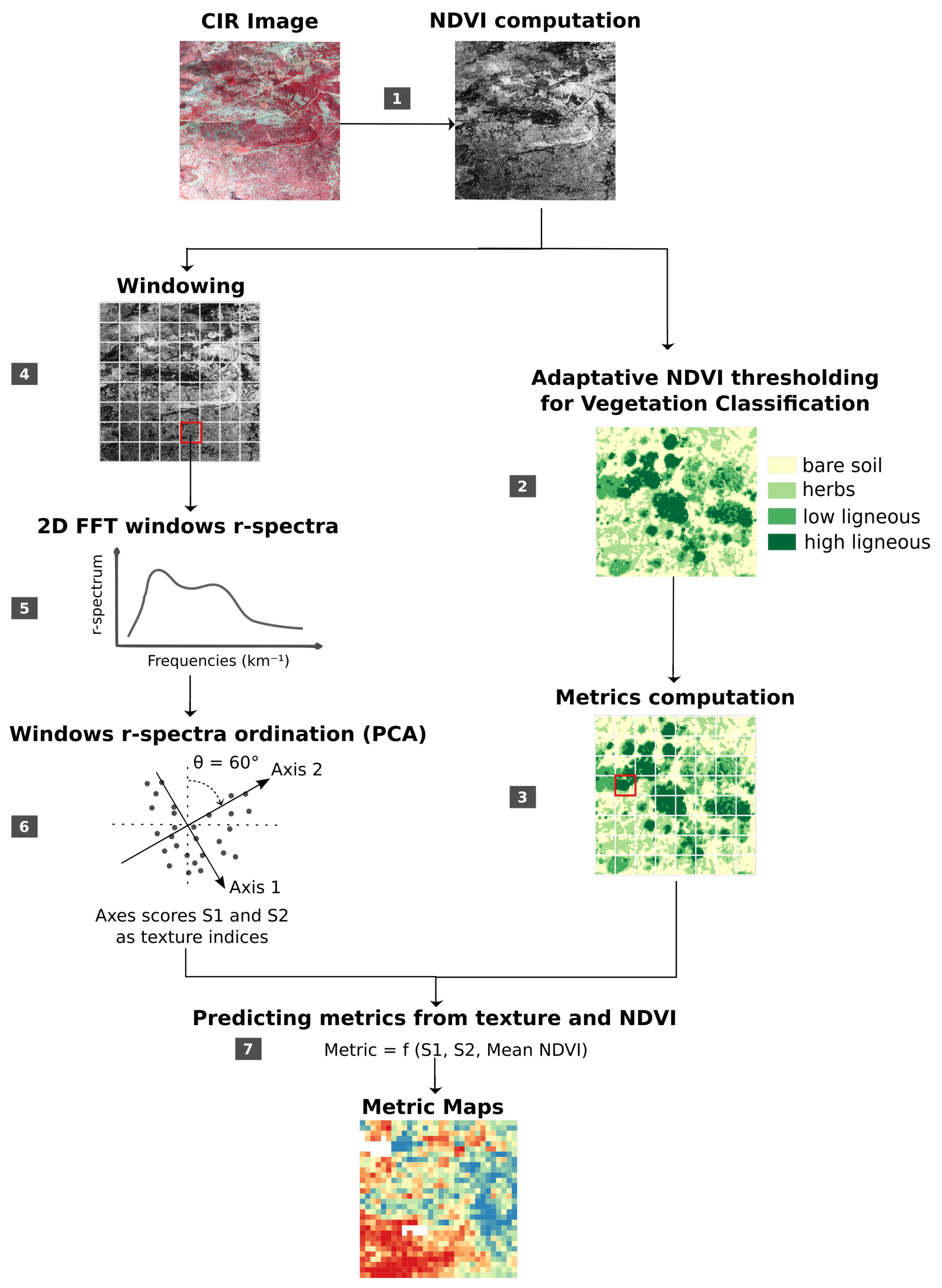
The general workflow of this study was built around the comparison of discrete and continuous approaches (Figure 1). First, the spatial distribution of the four strata of interest (BS, H, LL, and HL) was identified from very-high-resolution coloured infrared (CIR) airborne images based on radiometric differences among strata in the visible and near infrared domains [15] (Figure 1, step 1 and 2). We considered the four strata as pure and mutually exclusive. Next, we computed landscape structure metrics for individual vegetation strata and for grouped strata corresponding to ground strata (BS + H) and ligneous strata (LL + HL) considering homogeneous spatial units across the landscape (Figure 1, step 3). Then, we computed textural information from the Normalized Difference Vegetation Index (NDVI) layer of the CIR image (see Figure 1, steps 4–6). The textural information was obtained with the FOTO method, which is fully detailed bellow (Section 2.5). Finally, we tested the performances of the textural information as predictor variables for the estimation of landscape structure metrics when used with machine learning regression (Figure 1, step 7). Couteron et al. [37] highlighted that textural attributes lead to poor discrimination ability between landscapes with opposite structural patterns, such as patches of bare soil and herbaceous vegetation included in a matrix of dense ligneous vegetation vs. patches of dense ligneous vegetation included in a matrix of bare soil and herbaceous vegetation. It is thus suggested that the combination of textural attributes with radiometric information may improve the discrimination in this situation [37]. Therefore, here we considered the synergy between these two types of information by comparing the performance of models aiming at estimating landscape structure metrics when trained with textural and radiometric information separated or combined (Section 2.5.3).

2.1. Study Area

Mediterranean ecosystems are characterized by a complex landscape of heterogeneous mosaics. This heterogeneity is key to their exceptional level of biodiversity [5] and results from long-term co-evolution of human activities associated with heterogeneous semi-open habitats [38]. However, the structure of these natural habitats is currently shifting due to changes in traditional management practices, as mentioned previously. Among the many Mediterranean open habitats, the pseudo-steppe with grasses and annuals of the Thero-Brachypodietea [39] is threatened by the progressive encroachment of woody vegetation through natural successions due to the abandonment of grazing activities, and is also listed as a habitat of community interest by the European Council Directive 92/43/EEC, which aims to promote the maintenance of biodiversity. We focused on the site the Montagne de la Moure et Causse d’Aumelas, which is located in France, 30 km West of Montpellier (${43}^{\circ }{34}^{\prime }$N, $3^{\circ }{36}^{\prime }$N) (see Figure 2a). It is part of the European Natura 2000 ecological network for natural habitat conservation, and it was selected for our study because it contains numerous habitats of high interest organized in landscape mosaics, including pseudo-steppe with grasses and annuals of the Thero-Brachypodietea.

Our study site was a section of 3 km × 3 km (see Figure 2b) within Montagne de la Moure et Causse d’Aumelas. The area was carefully chosen to be representative of the diversity of vegetation types present on the whole site in order to test the generalizability of our approach. It is characterized by heterogeneous structure types, with a continuous openness gradient ranging from open pastures (e.g., Brachypodium retusum mixed with Thymus vulgaris) to degraded pastures with variable colonization rates of shrubs (Quercus coccifera, Juniperus oxycedrus, or Genista scorpius). There is a dynamic process of landscape closure by shrubs or forest (e.g., Quercus ilex and Quercus pubescens) (Figure 2c). The climate of this study site is characterized by hot dry summer with heavy rain events and a cold wet winter. Elevation is between 100 m and 349 m.

2.2. CIR Aerial Images

We used aerial images available through the BD ORTHO${}^{\circledR }$ IRC, a French CIR airborne image database. This image database, made available by the National Institute of Geographical and Forestry Information (IGN), is updated every three years and includes VHSR images (0.5-m spatial resolution) acquired over three spectral broad-bands with a radiometric resolution of 8 bits. These spectral bands correspond to the near-infrared, red, and green domains. It is a valuable source of information for vegetation structure at a fine scale over large areas at a reasonable cost [10,40]. The image dataset used in the study was acquired on the 23th and 26th of June 2012, respectively, between 1 and 2 p.m. and between 11 a.m. and 12 p.m., when the area of trees’ shadows was minimal. Vegetation seasonality is key to discrimination among strata: the photosynthetic activity of both herbaceous and ligneous strata in early vegetative season (spring) may reduce the ability of remote sensing to discriminate among these strata, while herbaceous vegetation dries first during early spring. Therefore, the period of image acquisition has a strong potential influence on the applications considered in this study. The data available for our study did not allow us to test the influence of seasonality, but the time of acquisition of our image dataset should reduce the risk of confusion between herbaceous and ligneous strata. Images are provided in 1 km${}^2$ square tiles downloadable in GeoTiff format, in Lambert-93 projection.

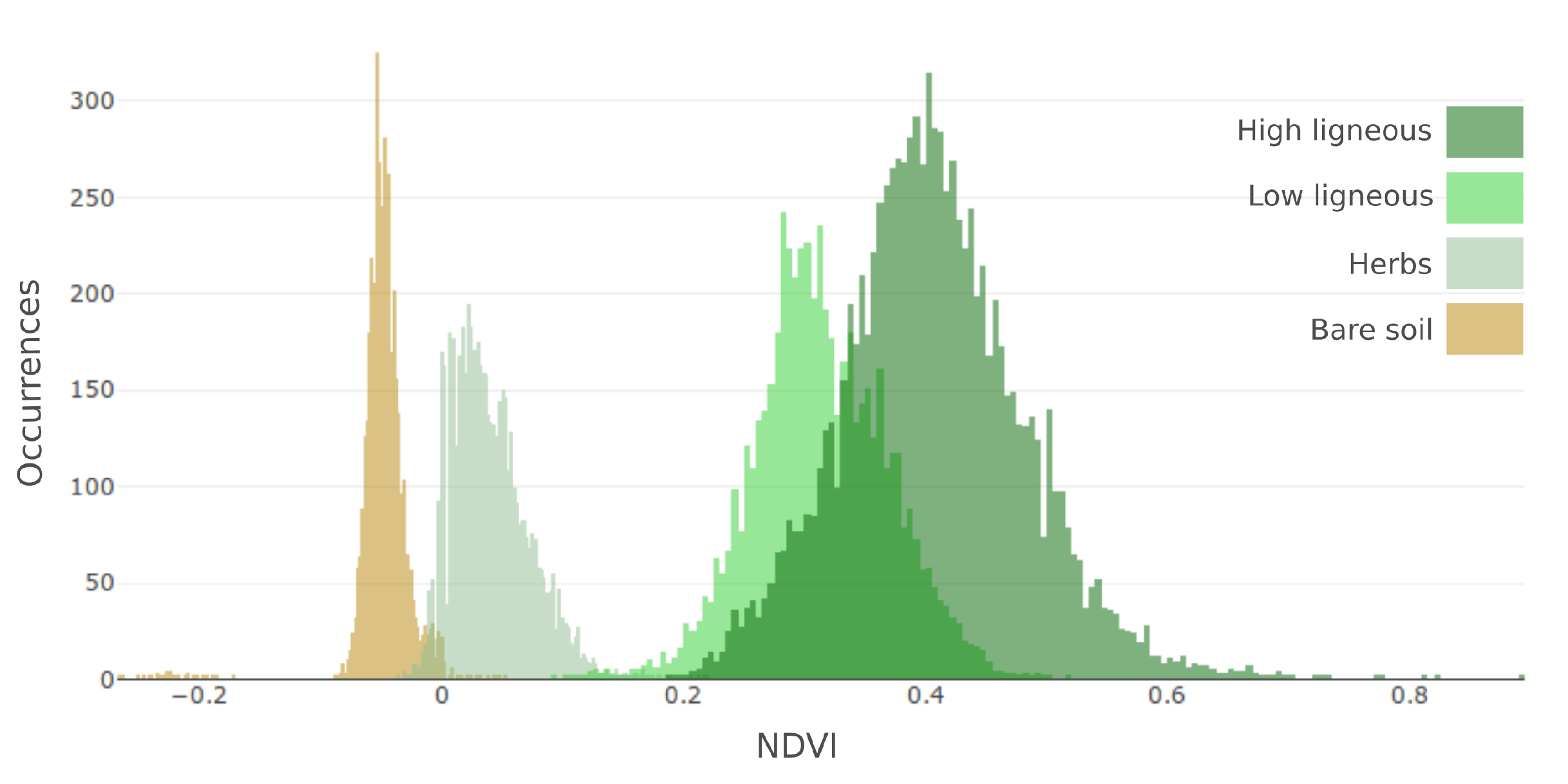
2.3. Identification of the Vegetation Strata

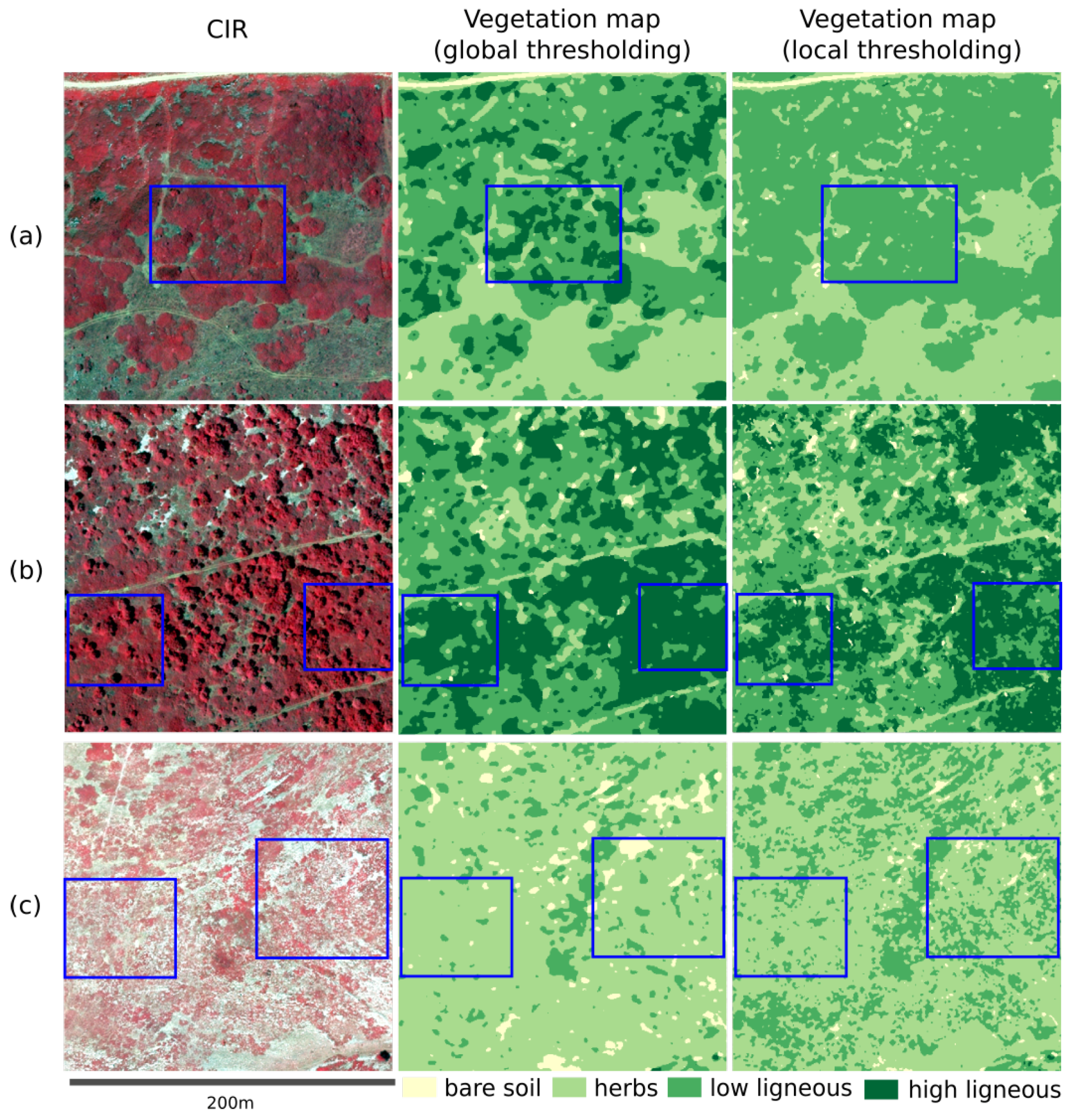
The distinction between the four vegetation strata was based on NDVI thresholding . NDVI is mainly used as an indicator of vegetation photosynthetic activity and vegetation density. Therefore, the choice of using it for the differentiation between BS and vegetated surfaces appeared particularly appropriate. Visual analysis of the NDVI images also highlighted that NDVI was relevant for the discrimination among vegetation strata, with NDVI values increasing with vegetation density, from H to LL to HL. However, the optimal threshold value allowing differentiating among strata varied substantially depending on the location on the site, leading to poor discrimination at the site scale when defining a unique threshold value to discriminate between pairs of strata.

We developed a graphical user interface in order to assist operators in the definition of the optimal local thresholds among strata based on visual interpretation. First, the image was split into 6.25 ha square windows. Then, thresholds between pairs of classes were defined sequentially—first between BS and H, then between H and LL, and finally between LL and HL. The presence of shadows may increase confusion when using NDVI as a criterion to discriminate among vegetation strata. We did not exclude shadows in our study, but image data was acquired around noon, in order to minimize these shadows. A $3\times 3$ majority filter was finally applied on the vegetation map prior to computation in order to remove the salt and pepper effect, considered here as an artefact of the classification process. We validated the resulting strata maps based on the identification of a set of regions by an independent operator. For each spatial unit and each stratum (if present), a set of regions with minimum surface of 2.5 m${}^2$ (i.e., 10 image pixels) with unambiguous identification was digitized after photo-interpretation and compared with the strata obtained from NDVI thresholding. In total, 524 regions representing 25,497 pixels (see

Table 1. Number of samples per vegetation strata digitized for assessment of the vegetation map validation. BS: bare soil; H: herbaceous vegetation; HL: high ligneous; LL: low ligneous.

Vegetation Strata	Number of Polygon Samples	Number of Pixels	Mean Number of Pixels per Polygon Sample
BS	132	4117	31
H	126	6170	49
LL	139	5576	40
HL	127	9634	76

) were identified. The accuracies of the global thresholding and the local thresholding methods were assessed using kappa coefficient, overall accuracy (OA), user accuracy (UA), and producer accuracy (PA) for each vegetation stratum.

2.4. Metrics Computation

Various landscape metrics were computed with FRAGSTATS 4.2.1. software. The metrics were computed with a specific window size N for each stratum or combination of stratum (BS + H and LL + HL) individually and for all strata considered together (called “landscape level” in FRAGSTATS). FRAGSTATS enables the computation of a large number of metrics for categorical landscape patterns. These metrics are grouped according to landscape pattern features. This study focused on three main groups, corresponding to area, shape, and aggregation metrics [26]. Some of these metrics show strong collinearity, in particular metrics from the same class [41,42]. In order to minimize redundancy and computational cost, a correlation analysis was performed to select a limited set of uncorrelated metrics from each group of metrics. The final selection resulted in one area metric, three shape metrics, and five aggregation metrics. Area metrics are related to the proportion of a stratum in the landscape with no information on its spatial distribution. Shape and aggregation metrics are related to landscape configuration; the former in terms of the complexity of patch shape, and the latter in terms of spatial aggregation of the same patch type.

Table 2. List of metrics used in the study.

Group	Acronym	Metric Name	Description
Area
	PLAND	Percentage of Landscape	Percentage of area occupied by a certain land cover class
Shape
	PAFRAC	Perimeter-Area Fractal Dimension	Patch shape complexity measure from 1 for shapes with simple perimeters to 2 for complex shapes
	SHAPE_MN	Shape Index Mean	Mean of patch shape irregularity. From 1 for square patches, increasing without limit with irregularity
	SHAPE_AM	Shape Index Area-Weighted Mean	Area-weighted mean of patch shape irregularity
Aggregation
	SPLIT	Splitting Index	Equal to the number of patches of a landscape divided into equal sizes, keeping landscape division constant
	IJI	Interspersion Juxtaposition Index	Measure of evenness of patch adjacencies, equals 100 for even and approaches 0 for uneven adjacencies
	AI	Aggregation Index	Measure of aggregation of a class: the percentage of neighbouring pixels being the same land cover class based on single-count method
	LSI	Landscape Shape Index	Ratio of the total edge to the minimum total edge
	COHESION	Patch Cohesion Index	Measure of the physical connectedness of the focal land cover class

lists all the selected indices of landscape patterns. The landscape metrics were computed with the vegetation classes delineated applying the eight neighbours rule. Each window was analyzed separately, and the window boundaries were not counted as edges.

2.5. Coarseness Gradient Computation

The textural gradients were generated with the FOTO method. FOTO combines two-dimensional Fourier transform and principal component analysis (PCA) techniques in order to ordinate image subsets according to their frequency content along a coarseness gradient [37]. First, a spatial sampling matching with the spatial sampling used to compute landscape metrics was performed, leading to elementary spatial units (or windows) of size N (Figure 1, step 4). Next, a Fourier transform was applied on each window and a radial spectrum (r-spectrum) was computed (Figure 1, step 5). Then, a PCA was performed and scores on the first prominent axes were used as textural indices after a loading rotation (Figure 1, step 6). In this study, the FOTO method was performed using the Matlab package used by Proisy et al. [43].

2.5.1. 2D Fast Fourier Transform and R-Spectra

Only broad outlines of the spectral analysis based on Fourier transform are provided here since many references describing the procedure are already available (e.g., [37,43,44,45]). First, the NDVI image was windowed into square windows of homogeneous size (Figure 1, step 4). Three percent of the study area corresponding to vineyard or tree plantations was masked, as they produce a very specific periodic pattern and bias the analysis. Then, a fast Fourier transform (FFT) was computed for each window of the original image. FFT aims at expressing the variance of an image as a weighted sum of cosine and sine waveforms of varying travelling direction and spatial frequency [37]. Following FFT, a periodogram I was computed for each window and defined by individual elements $I_{r\theta }$ corresponding to the portion of variance in NDVI explained by a given wavenumber r and travelling in direction $\theta$ [45]. The wavenumber is defined as the number of times a waveform signal is repeated in the window’s travelling direction $\theta$ [37]. For each spatial frequency, an azimuthally averaged radial spectrum (r-spectrum) $I\left(r\right)$ was produced by averaging values on all travelling directions (Figure 1, step 5).

FOTO provides a convenient way to quantify coarseness-related properties with no prior directional assumption by studying the decomposition of variance among spatial frequencies, and proved to be useful for analyzing landscape patterns [37]. We expressed wavenumber as spatial frequencies f in cycles per kilometer.

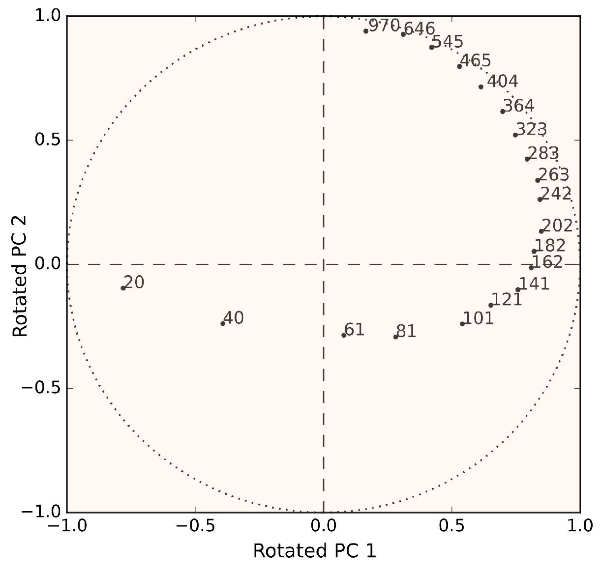
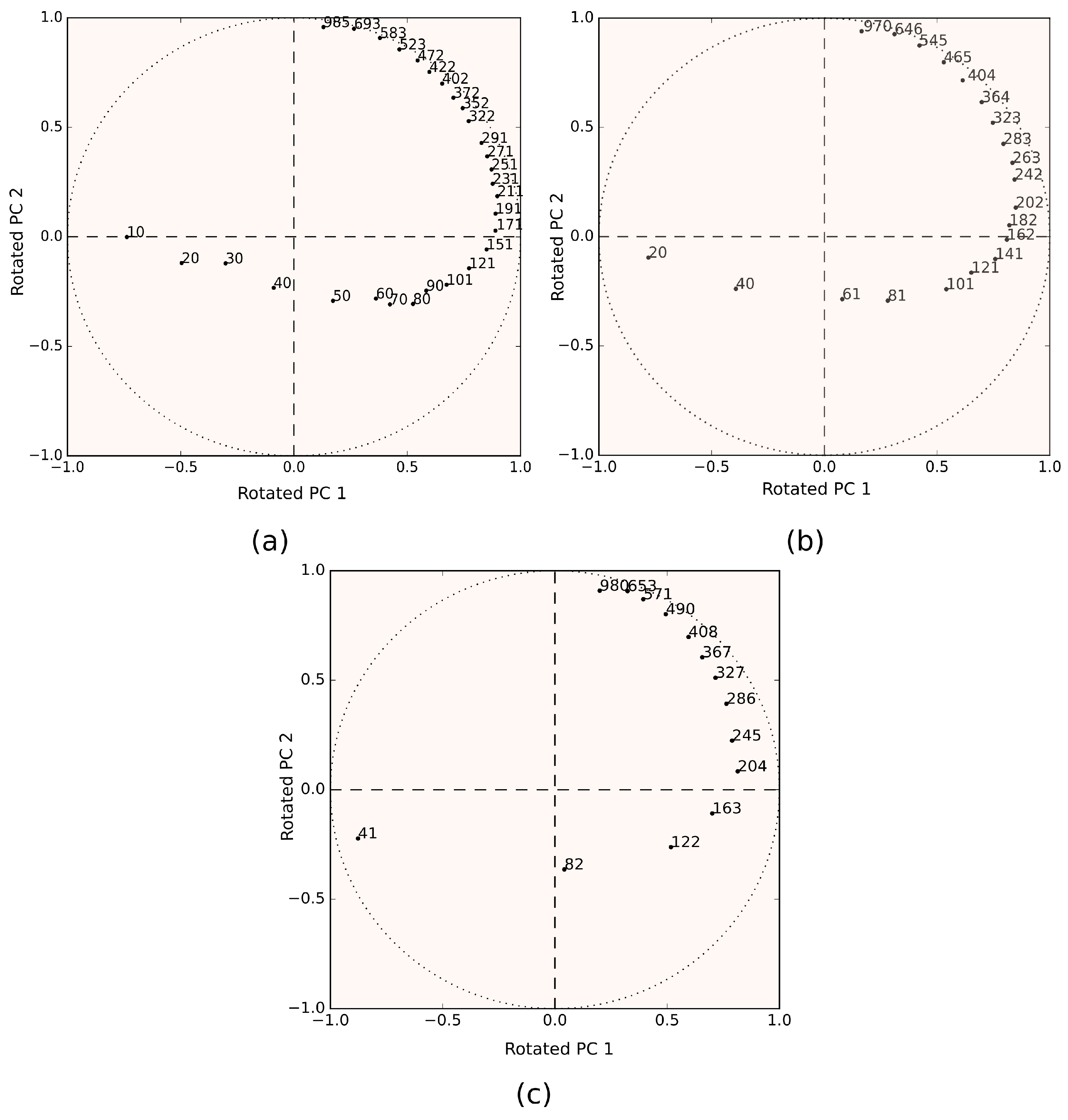
2.5.2. Textural Ordination

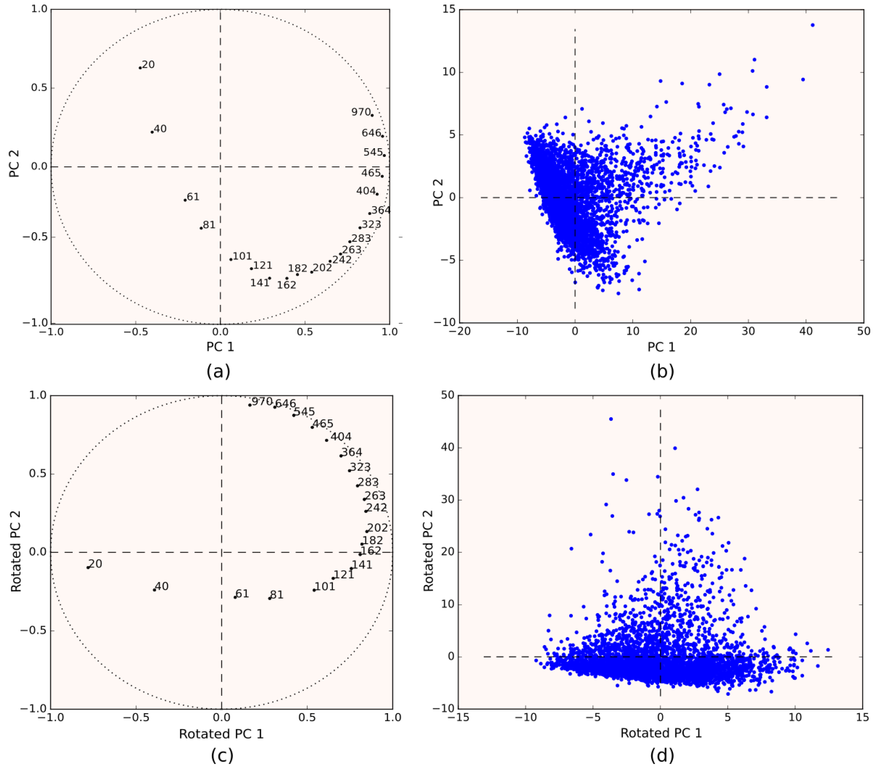
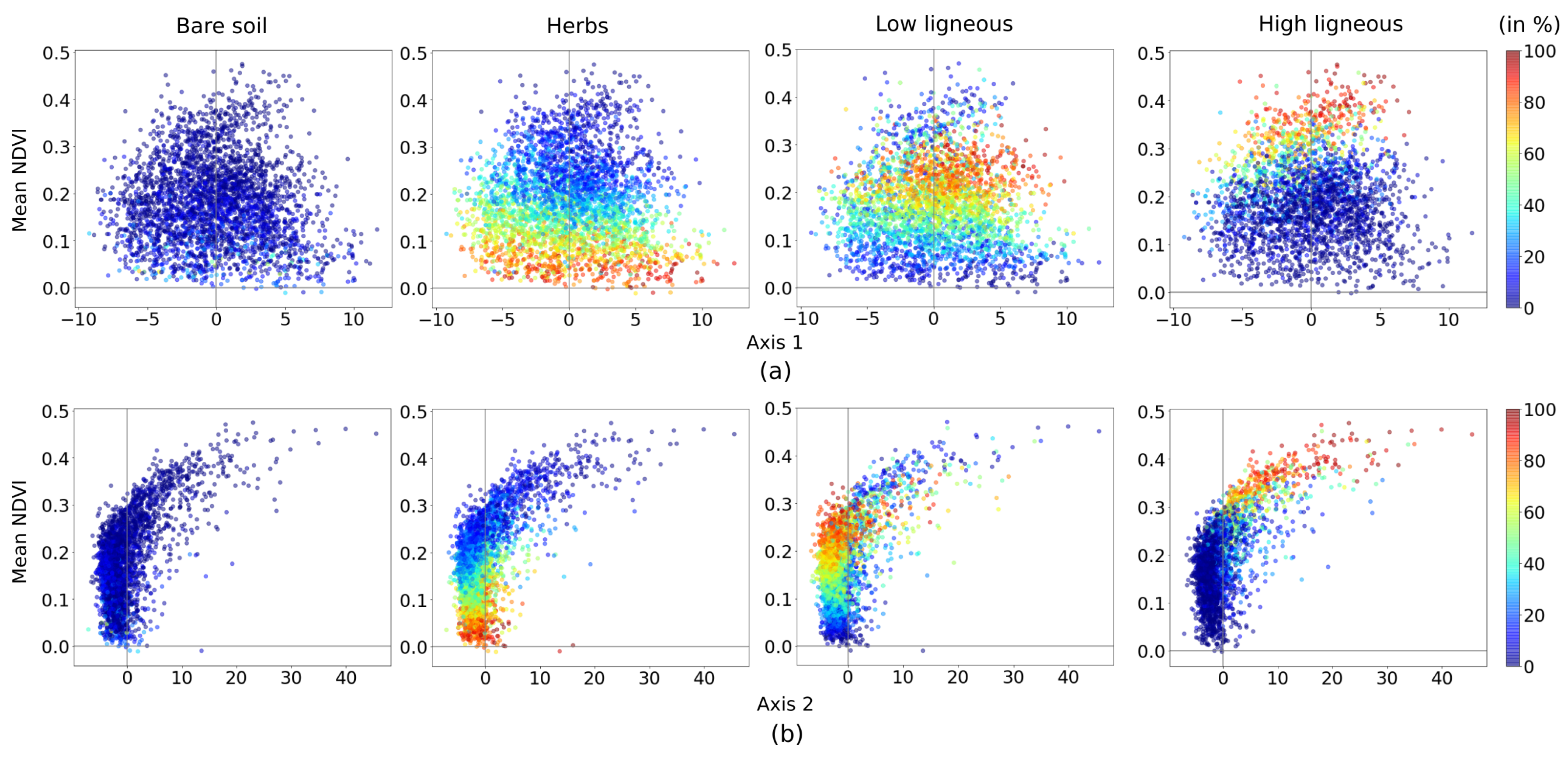
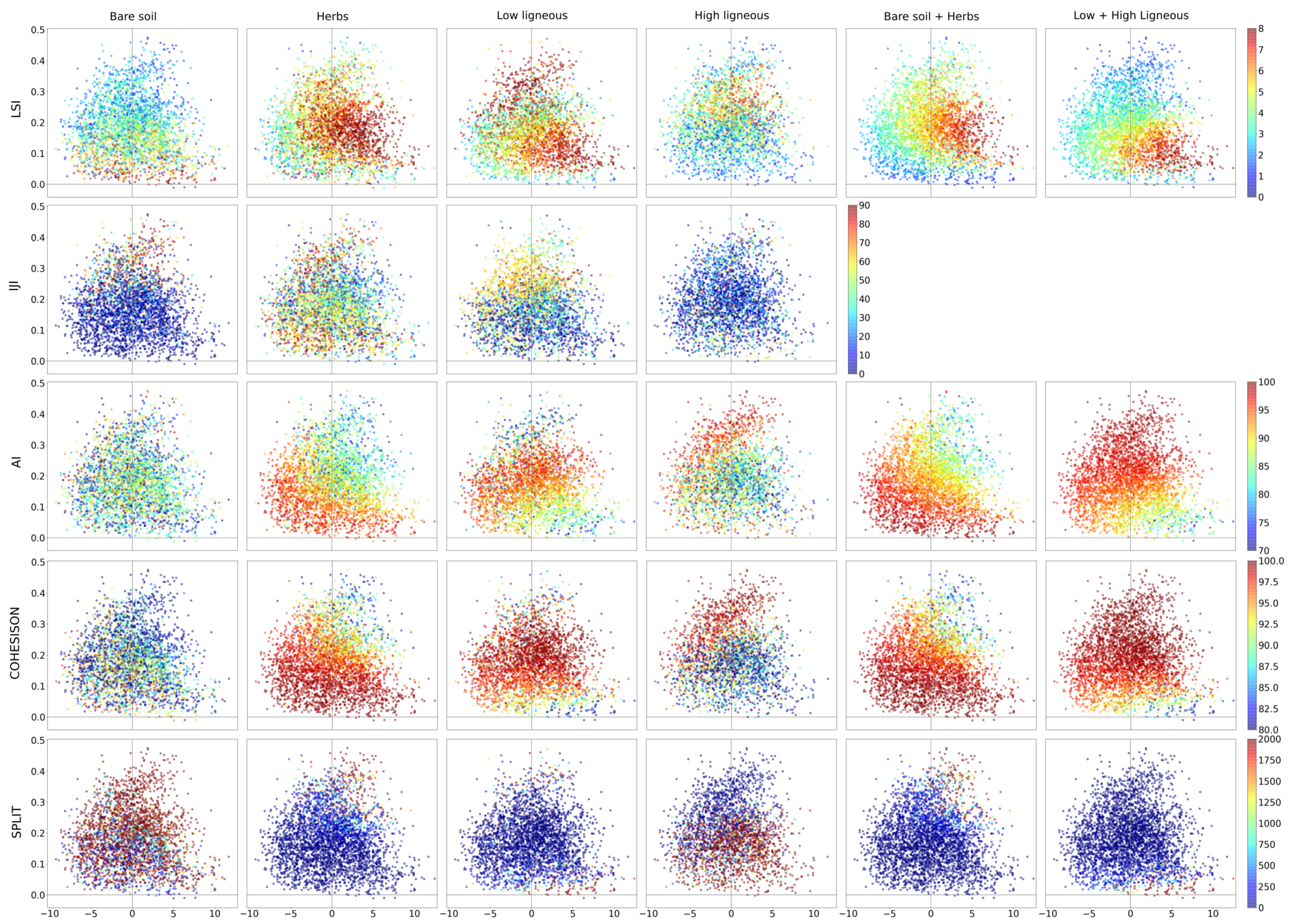
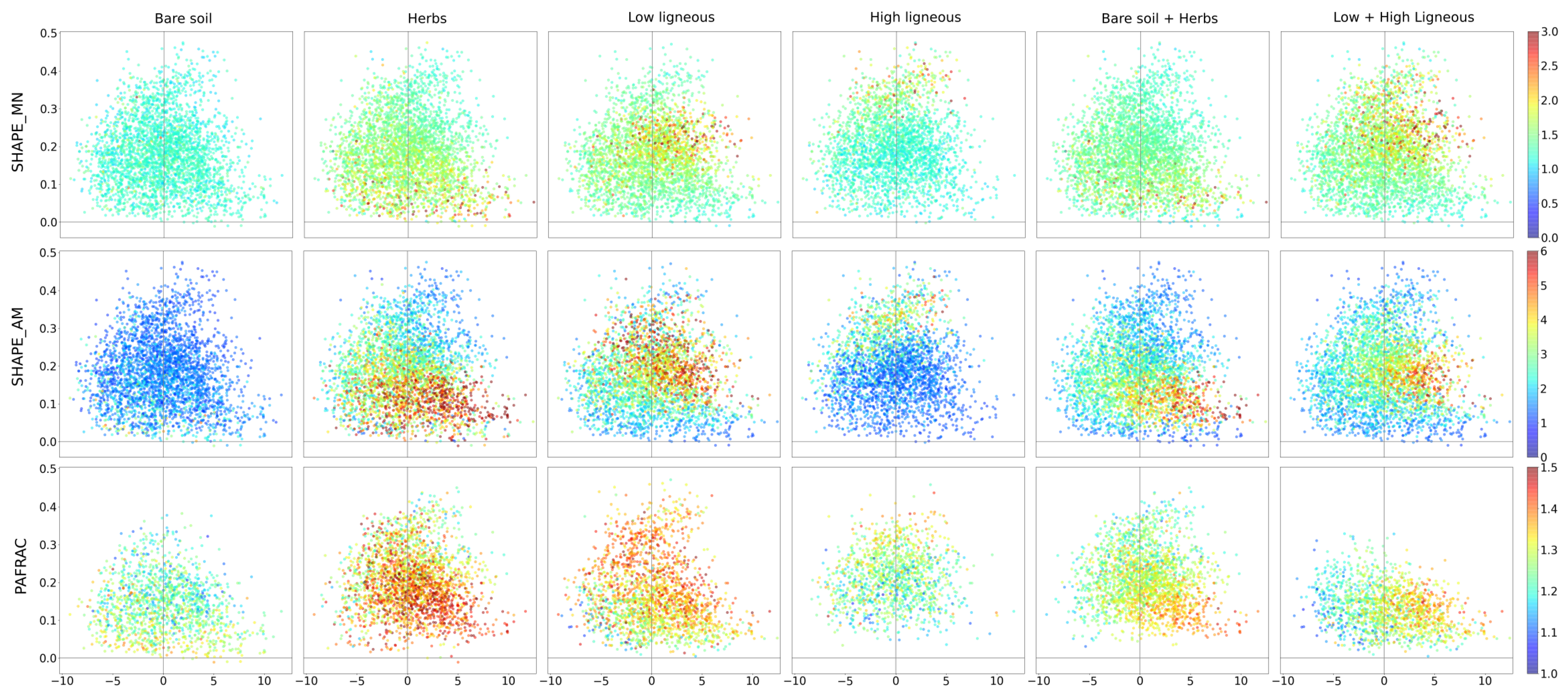
A table compiling the r-spectra was produced, each row corresponding to the r-spectrum of a given window, and each column corresponding to a spatial frequency. Then, a PCA was applied to this table [46]. The table was standardized prior to PCA in order to avoid excessive influence of low spatial frequencies [37]. The main axes resulting from the PCA could be linked to the texture, and the first two are usually related to the following orthogonal coarseness gradients in the literature [37,43]: the first axis usually corresponds to a coarseness gradient that evidences the contrast between coarse texture and fine/very fine texture, and the second axis to another coarseness gradient evidencing the contrast between intermediate–coarse texture and very coarse or very fine texture. 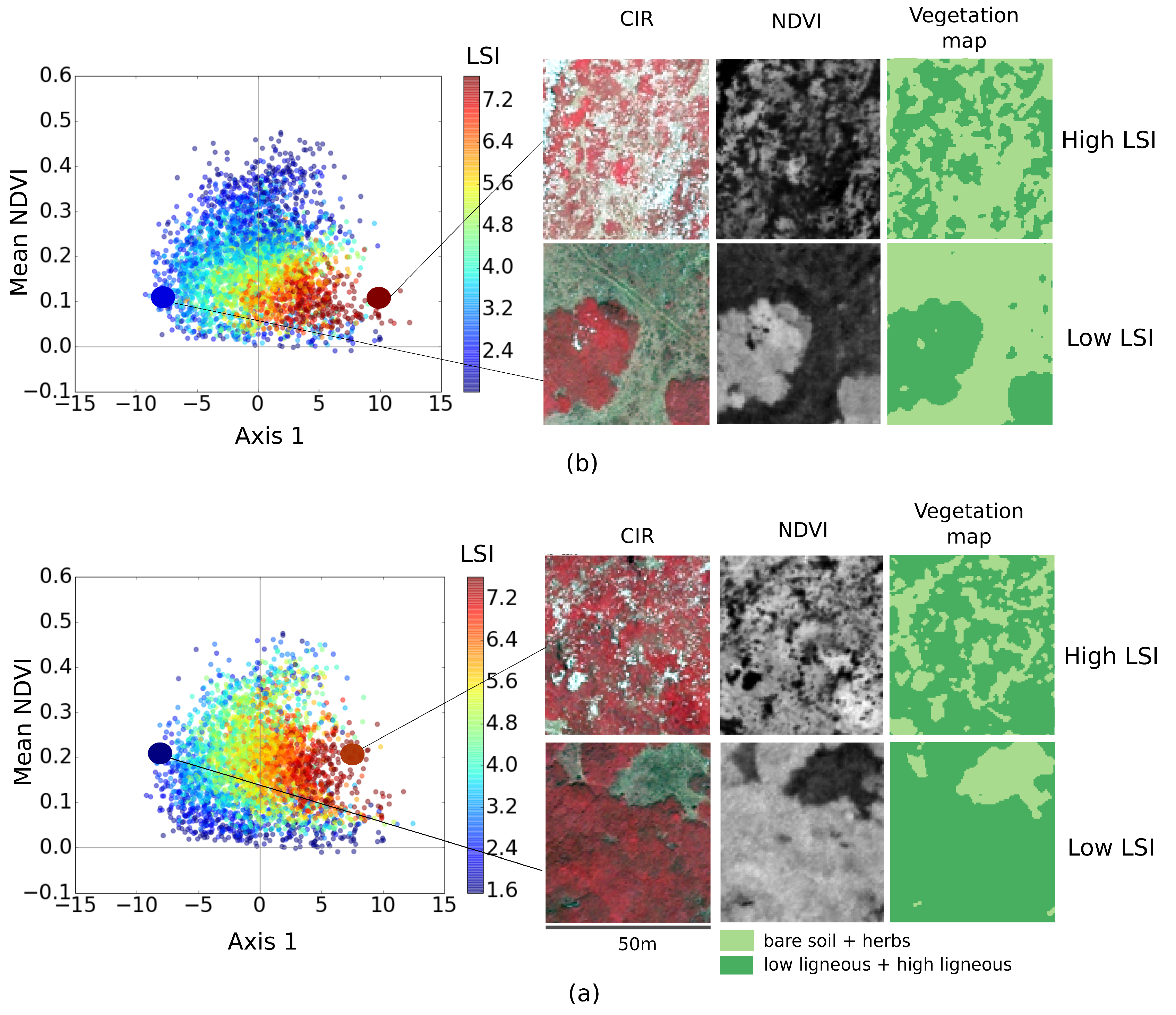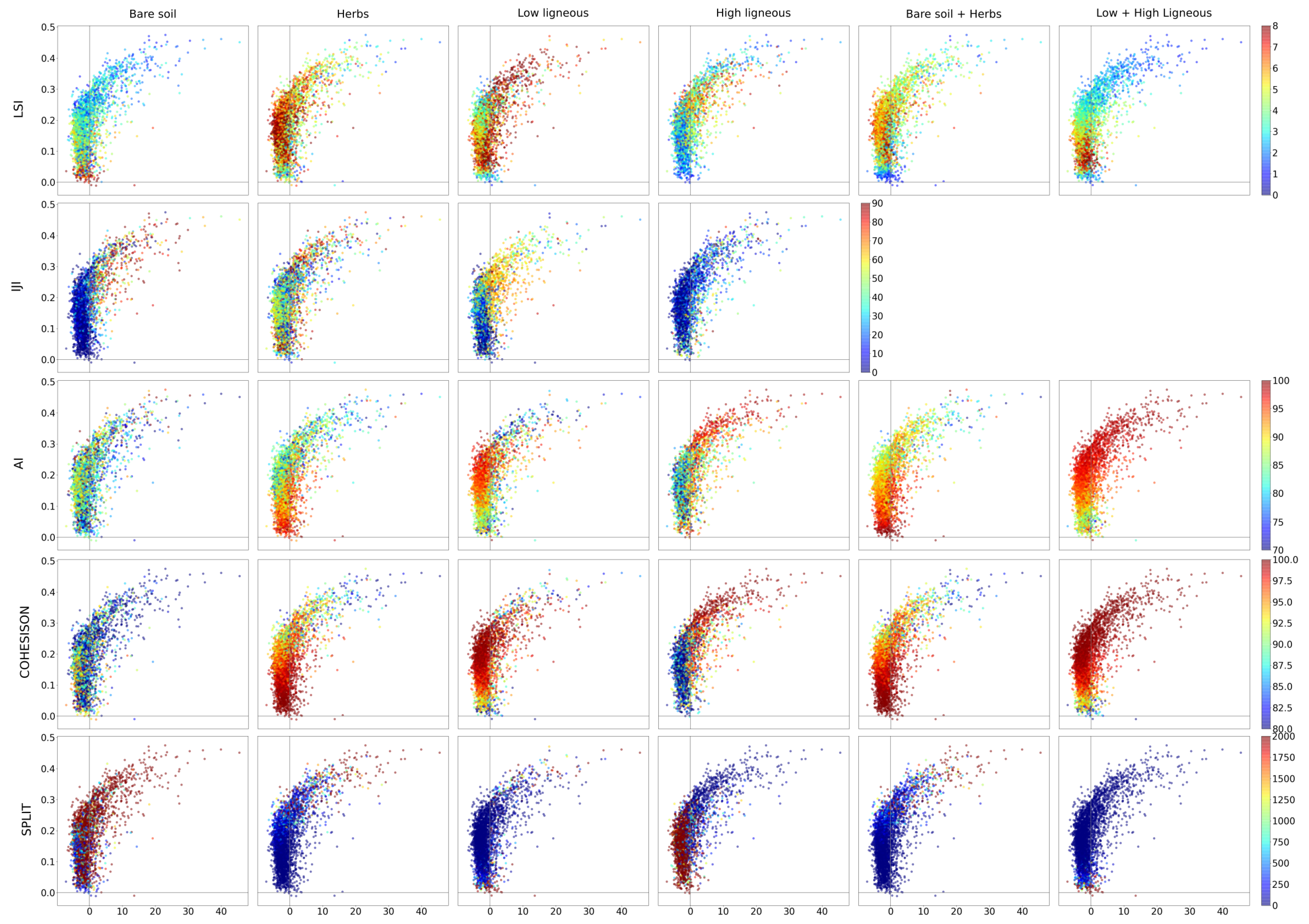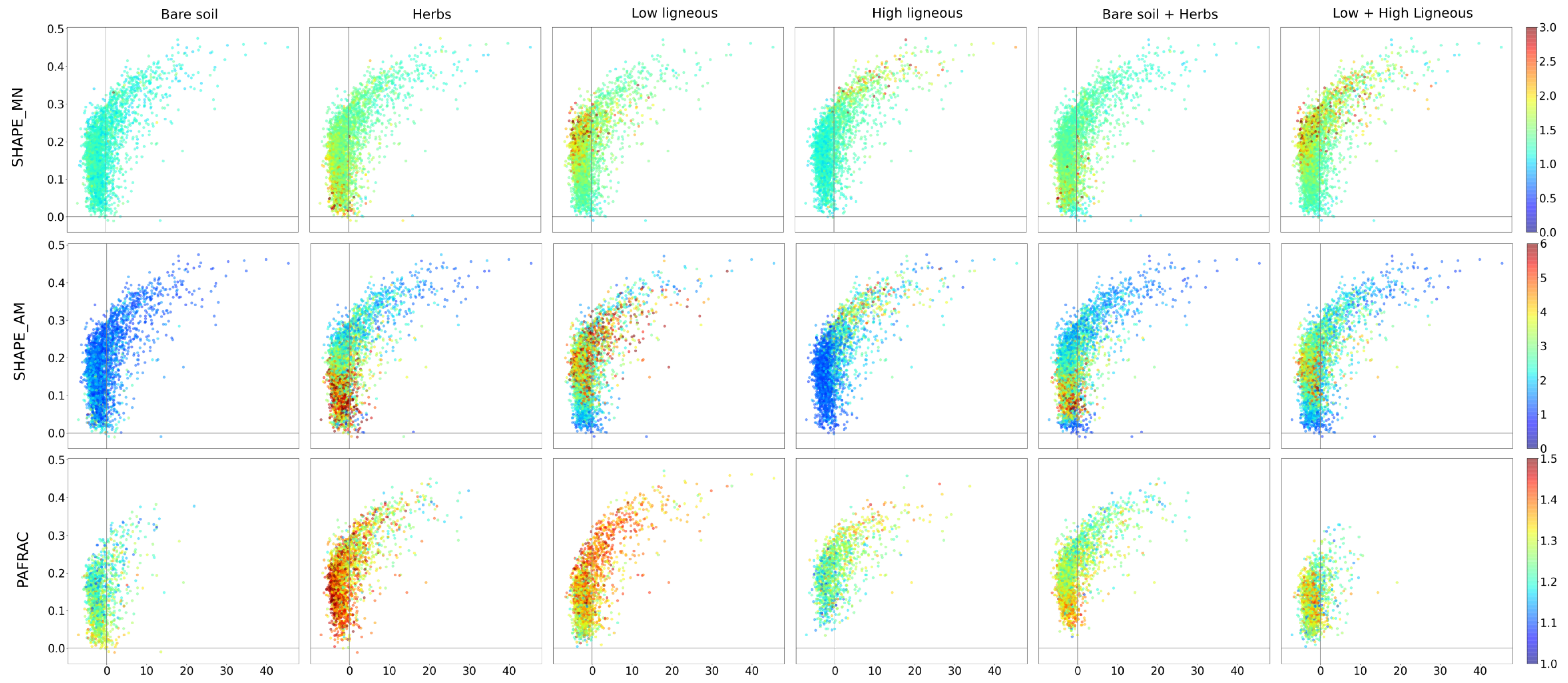Fine and very fine textures are generally linked to densely forested areas due to canopy grain, and the first gradient described previously is particularly useful when linking textural metrics with canopy structure of Amazonian forests [47] or development stages in dynamic mangroves [43]. However, when studying the semi-open landscapes, the forest can be considered as secondary compared to intermediate–coarse or fine texture linked to patterns made by patches of dense ligneous vegetation included in a matrix of bare soil and herbaceous vegetation. In that respect, the first gradient was not the most relevant in the context of this study. Therefore, in order to simplify the interpretability of our results, we performed an orthogonal rotation aiming at defining a new first axis, evidencing the contrast between very coarse and intermediate or fine texture, which was thus better related to semi-open landscape structure.

The rotated axes remain orthogonal and explain the same global amount of variance as the initial coarseness gradients. However, as the rotation was performed for optimal interpretation, and the definition of the first rotated axis is arbitrary and application dependent, the variance explained by the first rotated axis may be lower than the variance explained by the second rotated axis.

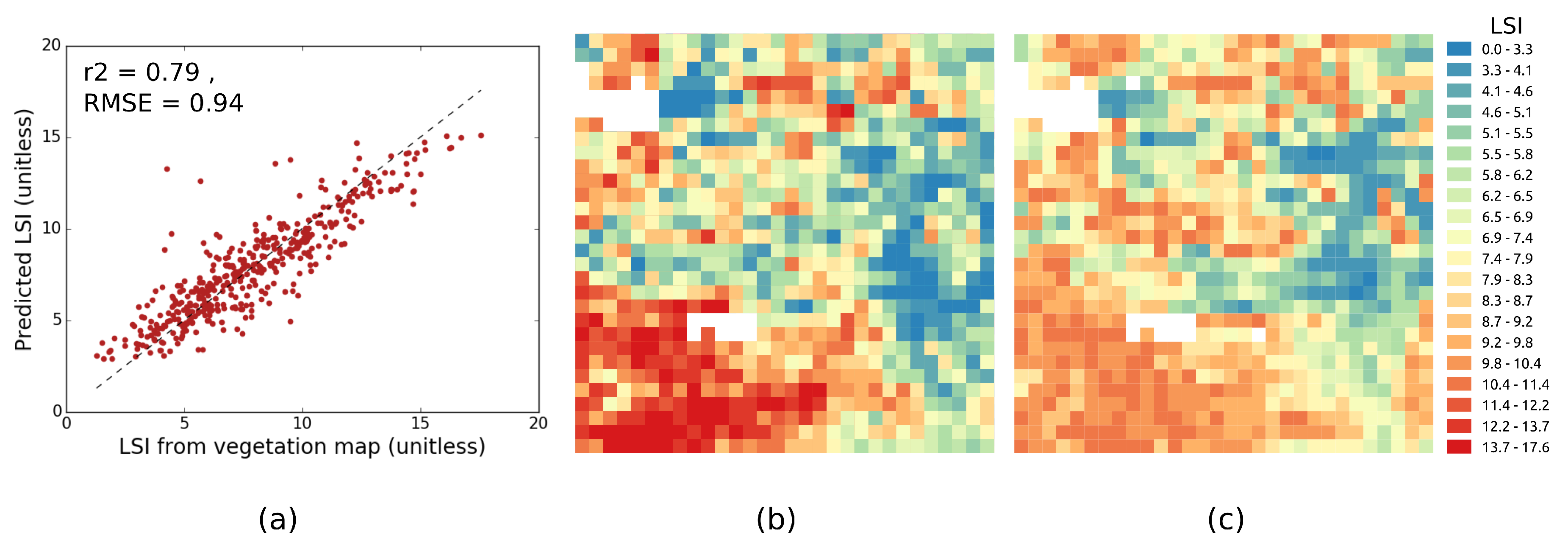
2.5.3. Coupling FOTO Outputs with Landscape Metrics

In the final step of the process, the ability of textural information and radiometric information to predict landscape metrics was tested with regression models based on support vector machine (SVM). We used a nonlinear radial basis function kernel. The regression involved three steps. First, the full dataset was split into a training dataset and a validation dataset, and the optimal values of the free parameters of the SVM (cost (C) and gamma ($\gamma$)) were identified based on an exhaustive grid search strategy with cross-validation on the training dataset. The space defined by values ranging from $2^{-2}$ to $2^3$ was explored for both parameters. Then, the model was trained with the full training dataset and C and $\gamma$ set to their optimal values defined in the first step. Finally, the resulting mode was applied on the validation data set. 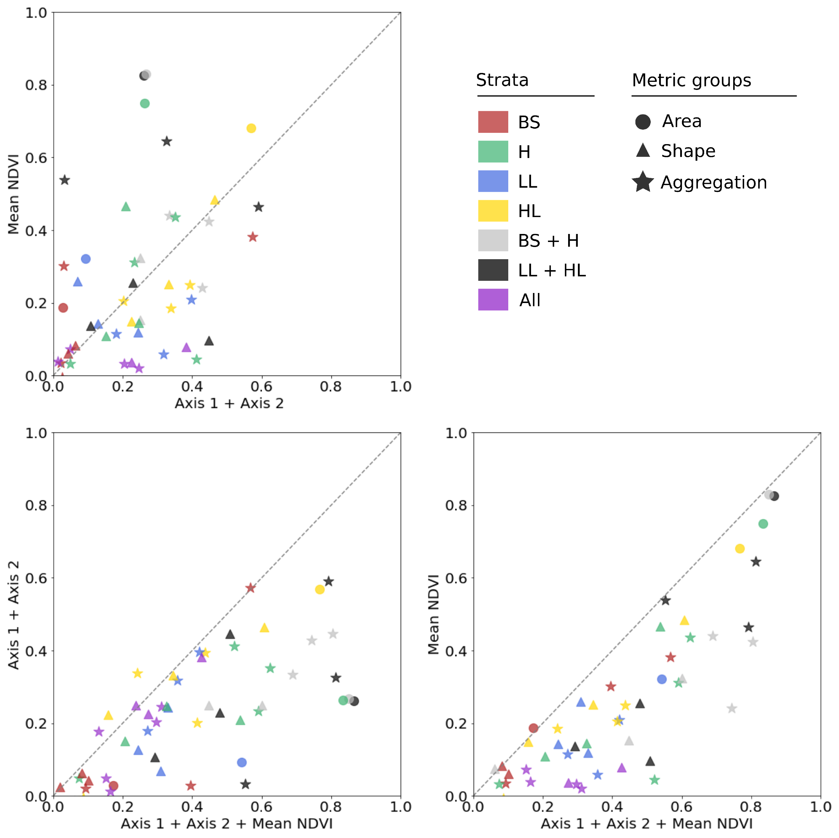We used the coefficient of determination (Equation (1)), with $y_i$ the measured values, ${\widehat{y}}_i$ the predicted values, and ${\overline{y}}_i$ the mean of measured values as fitness quality criterion for the models.

In order to test the synergy between the mean NDVI and FOTO indices, we adjusted regression models based on the two first rotated axes obtained from FOTO only, mean NDVI only, and the combination of the two first rotated axes and the mean NDVI. Indeed, the Fourier decomposition is insensitive to opposite patterns in terms of radiometric information: patches of bare soil and herbaceous vegetation included in a matrix of dense ligneous vegetation may show the same textural information as patches of dense ligneous vegetation included in a matrix of bare soil and herbaceous vegetation [37]. Thus, two windows can have similar coarseness attributes but very different vegetation structure. Here, each metric was predicted from three different sets of variables: FOTO indices only, mean NDVI only, and a combination of both FOTO indices and mean NDVI. Regression models were finally used to spatially predict landscape metrics and produce a spatial representation of these landscape metrics.

$$r^2=1-\sum _{i=1}^n\frac{{(y_i-{\widehat{y}}_i)}^2}{{(y_i-{\overline{y}}_i)}^2}$$

(1)

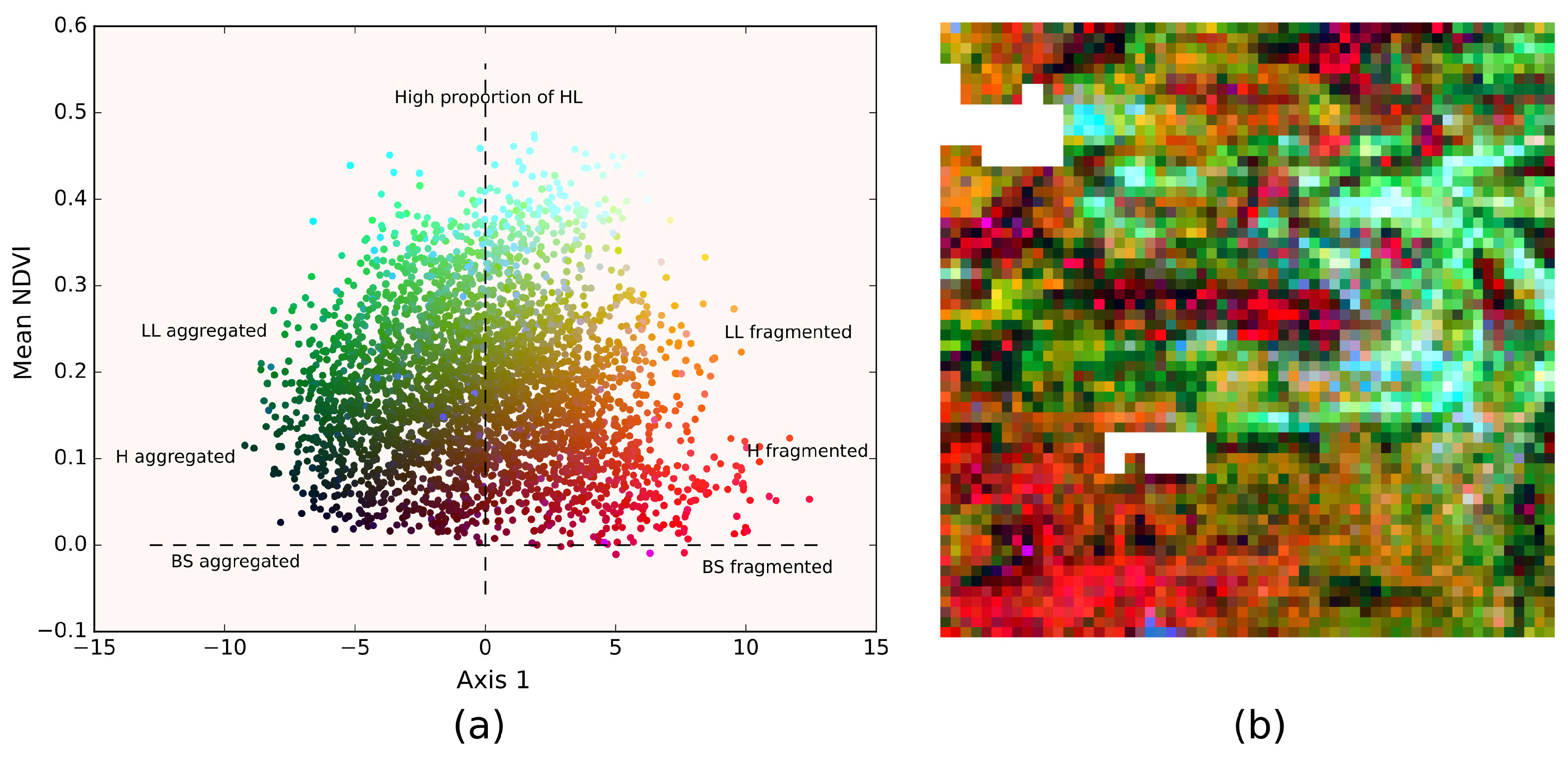
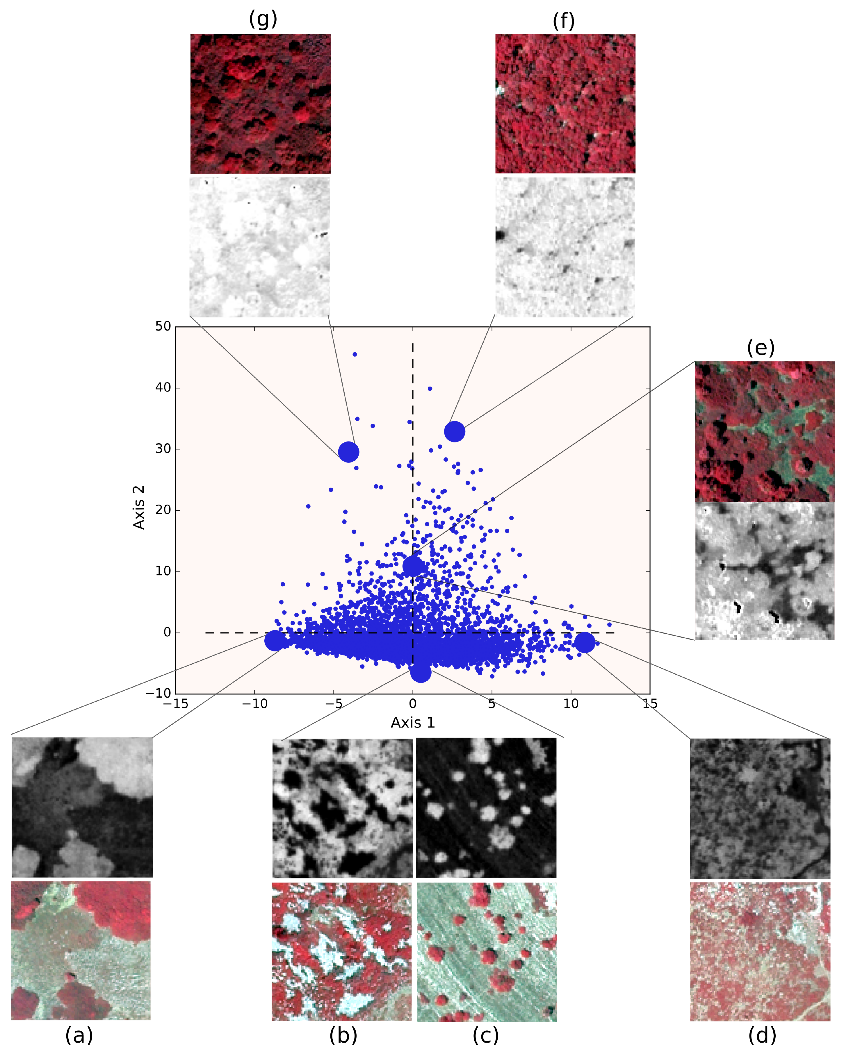
2.5.4. Mapping FOTO Indices Enhanced with Mean NDVI

We tested the potential of the combination of textural ordination and radiometry as a straightforward tool for characterizing vegetation organization with synoptic representations. We hence represented the two first rotated components of PCA and the mean NDVI as a composite red–green–blue image [43], with the colours corresponding to window scores for the first rotated axis, the mean NDVI value, and the second rotated axis respectively.

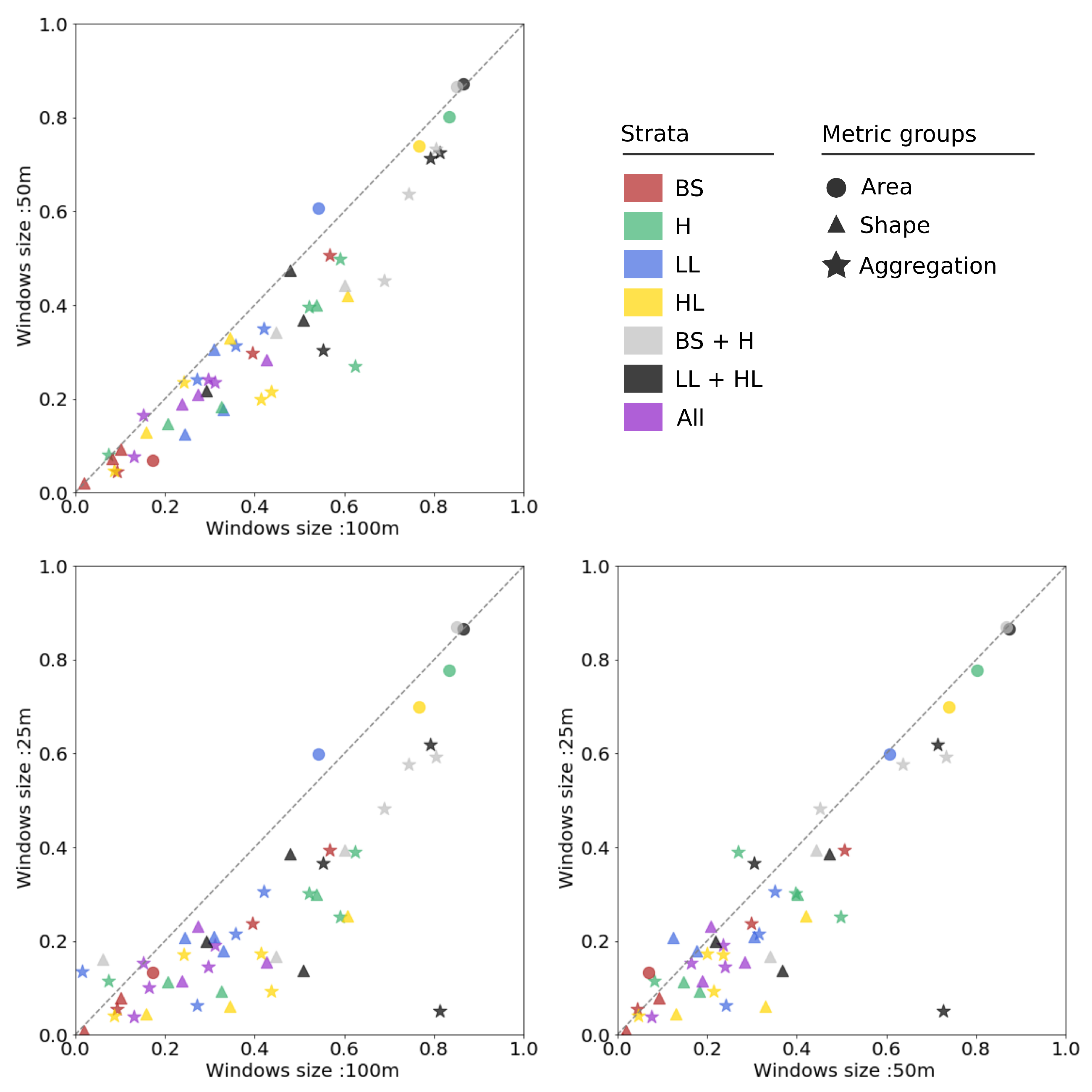
The spatial resolution of the resulting maps corresponds to the window size used for the FOTO analysis and the computation of the landscape metrics. Increasing the spatial resolution of the maps to get more spatial details on vegetation organization implies reducing the window size for FOTO analysis and thus not taking into account low spatial frequencies that may be of interest for the characterization of vegetation strata structure. As window size is a compromise between spatial resolution of textural maps and the number of frequencies included in the analysis, we tested the influence of three different window sizes on the synoptic landscape maps: 25 m, 50 m, and 100 m.

3. Results

3.1. Classification Results

Classification using global thresholds showed an overall accuracy of 86.9% and a Kappa Coefficient of 0.818 (

Table 3. Confusion matrix of the vegetation map of the following the strata : bare soil (BS), herbs (H), low ligneous (LL), and high ligneous (HL). The classification was computed with with unique threshold values for the whole scene.

Reference Data	Classification Results
	BS	H	LL	HL	Producer Accuracy	Number of Pixels
BS	3884	293	0	0	0.93	4177
H	36	6106	28	0	0.99	6170
LL	0	27	3495	2054	0.63	5576
HL	0	0	899	8735	0.91	9634
User accuracy	0.99	0.95	0.79	0.81

Overall accuracy (OA): 0.869; KAPPA: 0.818.

), with accurate identification of BS and H, whereas strong confusion between strata LL and HL was observed (37% of LL pixels misclassified into HL). This was expected given the distribution of NDVI for each class illustrated in Figure 3. The confusion between LL and HL was strongly reduced (commission error reduced to 14%) when using local thresholding (

Table 4. Confusion matrix of the vegetation map of the following the strata : bare soil (BS), herbs (H), low ligneous (LL), and high ligneous (HL). The classification was computed with locals thresholds.

Reference Data	Classification Results
	BS	H	LL	HL	Producer Accuracy	Number of Pixels
BS	3839	330	0	8	0.92	4177
H	54	6043	62	11	0.98	6170
LL	0	146	4673	757	0.84	5576
HL	0	6	1630	7998	0.83	9634
User accuracy	0.99	0.93	0.73	0.91

Overall accuracy (OA): 0.882; KAPPA: 0.839.

). However, the overall accuracy remained relatively similar. The definition of the LL stratum was particularly improved with local thresholding. Logically, the classification accuracy reached more than 99% classification accuracy when combining H with BS, and LL with HL (

Table 5. Confusion matrix of the vegetation map of the grouped classes bare soil and herbs (BS + H) and ligneous (LL + HL). The classification was computed with unique threshold values for the whole scene.

Reference Data	Classification Results
	BS-H	L	Producer Accuracy	Number of Pixels
BS + H	10,319	28	0.99	10,347
LL + HL	27	15,183	0.99	15,210
User accuracy	0.99	0.99

Overall accuracy (OA): 0.998; KAPPA: 0.996.

and

Table 6. Confusion matrix of the vegetation map of the grouped classes bare soil and herbs (BS + H) and ligneous (LL + HL). The classification was computed with locals thresholds.

Reference Data	Classification Results
	BS-H	L	Producer Accuracy	Number of Pixels
BS + H	10,266	81	0.99	10,347
LL + HL	152	15,058	0.99	15,210
User accuracy	0.99	0.99

Overall accuracy (OA): 0.991; KAPPA: 0.981.

).

3.2. Interpretation of R-Spectra Ordination

The interpretation of the r-spectra was performed for a specific window size of 50 m in order to allow image subsets with more homogeneous frequency content and then facilitating the illustration of r-spectra ordination. PCA resulted in two principal axes accounting for 82% of the total variability of the r-spectra computed over the full landscape. A rotation of ${60}^{\circ }$ was applied on these two axes in order to optimize the interpretation of the coarseness gradients produced by FOTO. Bellow, only the results for rotated axes are detailed, but further details on rotation can be found in the Appendix B (see Figure A5).

The first rotated axis explained 27% of the total variability (Figure 4). It evinced a contrast between low (less than 40 cycles km${}^{-1}$) and intermediate frequencies (greater than 120 cycles km${}^{-1}$). That is, windows containing a higher share of the variance accounted for by low frequencies had a low score on axis 1 and windows containing a higher share of the variance accounted for by intermediate frequencies had a high score on axis 1 (Figure 4). The second rotated axis explained 55% of the total variability of the r-spectra. This axis evinced a contrast between low and intermediate (less than 200 cycles km${}^{-1}$) and high frequencies (greater than 320 cycles km${}^{-1}$).

The correspondence between landscape structure and position along the two rotated axes is illustrated in Figure 5. The selection of image subsets distributed along increasing values for the first axis and low values for the second axis highlight the transition from:

• coarse patterns corresponding to macro heterogeneity at window-scale, that is, patterns too large to be evinced at window-scale and resulting in windows partitioned by a few patches of vegetation such as edges between H and large mats of LL (Figure 5a);
• to intermediate patterns corresponding to LL mixed with H or BS (Figure 5b,c);
• to fine patterns due to highly mixed LL and H strata—a structure characteristic of the degradation of habitats such as the pseudo-steppe with grasses and annuals of the Thero-Brachypodietea habitat (Figure 5d).

The selection of image subsets distributed along increasing values for the second axis highlights a coarseness gradient ranging from the structures described for the first axis (low values on second axis), to image subsets containing finely textured groups of trees embedded in a matrix of coarser texture corresponding to BS, H, and LL strata (Figure 5e, intermediate values on second axis), to image subsets characterized by very fine texture overall corresponding to closed canopies, with possible differences among canopy structures along the first axis (Figure 5f,g, higher values on second axis). As shown in Figure 5b,c, two windows with similar coarseness attributes in terms of coarseness defined by the two axes may show very different vegetation structure because of the insensitivity of Fourier decomposition to mean radiometric information. These results show that the first axis was a relevant descriptor of the succession of different strata (inter-strata heterogeneity), whereas the second axis showed structures corresponding to windows mainly occupied by the HL strata (intra-strata heterogeneity).

3.3. Linking Textural Gradient with Landscape Metrics

3.3.1. Predicting Landscape Metrics from FOTO Indices

SVM models were adjusted in order to estimate several landscape metrics from the values along the two first axes, and the corresponding coefficients of determination are detailed in

Table 7. Coefficient of determination $r^2$ of regression models predicting landscape metrics for each strata from texture axis 1 and texture axis 2, for a window size = 100 m. Empty space means that metrics could not be computed for the corresponding strata or combination of strata.

Metrics Strata	Area	Shape			Aggregation
	PLAND	PAFRAC	SHAPE_MN	SHAPE_AM	SPLIT	IJI	AI	LSI	COHESION
BS	0.03	0.06	0.03	0.04	−0.65	0.57	0.03	0.03	0.02
H	0.26	0.25	0.15	0.21	−0.25	0.05	0.23	0.41	0.35
LL	0.09	0.24	0.13	0.07	−3.20	0.40	0.18	0.32	−0.14
HL	0.57	0.22	0.33	0.46	−0.85	−0.00	0.39	0.20	0.34
BS + H	0.27	0.25	−0.01	0.25	−0.14		0.45	0.43	0.33
LL + HL	0.26	0.45	0.11	0.23	−0.63		0.32	0.59	0.03
All		0.25	0.22	0.38	0.01	0.18	0.25	0.20	0.05

. These results correspond to a window size of 100 m, because the best prediction power of the textural indicator was found for this window size. The influence of window size is discussed in the following section. The regression models for the estimation of the area metric (percentage of landscape occupied by a given strata, PLAND) showed poor performances, with $r^2$ less than 0.27 for all strata, except for HL with $r^2=0.57$. The regression models for the estimation of the shape and aggregation metrics showed higher performances for grouped strata than for individual strata: the coefficients of determination between landscape metrics derived from the grouped stratum HL + LL and corresponding estimation based on textural indices reached 0.45 and 0.59 for perimeter-area fractal dimension (PAFRAC) and landscape shape index (LSI) respectively, whereas it reached 0.24 and 0.32 when computed for stratum LL only, and 0.22 and 0.20 when computed for stratum HL only. Indeed, only four models resulted in predictions with $r^2$ higher than 0.40, corresponding to the estimation of the following metrics: SHAPE_AM (shape index area-weighted mean) for stratum HL (0.46), LSI for stratum H (0.41), interspersion juxtaposition index (IJI) for stratum BS (0.57), and IJI for stratum LL (0.40). The models adjusted for the estimation of the splitting index (SPLIT) showed particularly poor performances, and negative $r^2$ values were obtained, which means that models fitted more poorly than a model predicting a constant value.

3.3.2. Synergy of NDVI and Textural information

Regression models were then adjusted based either on mean NDVI value, or on the combination of mean NDVI and textural indices computed from each 100 m individual window, and the performance of the three types of models (texture-based, mean NDVI-based, and combined) were compared (Figure 6). Models with only mean NDVI used as predictor variable showed higher values of coefficient of determination than the models adjusted with textural indices as predictor variables for area metrics, with particularly high values for H, HL, and grouped strata ($r^2>0.6$). On the other hand, NDVI-based models were outperformed by texture-based models for the estimation of shape and aggregation metrics for most of the strata.

The models combining textural gradients and mean NDVI as predictor variable systematically led to equivalent or increased values of coefficient of determination when compared to models using the two types of information separately. In the case of area metrics, the combination of two types of information resulted in a noticeable increase of $r^2$ compared to NDVI only, for the LL stratum only. In the case of aggregation and shape metrics, the agreement between metrics derived from discrete approaches and estimated from the combination of texture and NDVI was strongly improved for most of the grouped strata, and to a lesser extent for individual strata.

Detailed results of regression models based on textural information and NDVI corresponding to window size of 100 m are presented in

Table 8. Coefficient of determination $r^2$ of regression models predicting landscape metrics for each strata from texture axis 1, texture axis 2, and mean NDVI, for window size = 100 m. Empty space means that metrics could not be computed for the corresponding strata or combination of strata.

Metrics Strata	Area	Shape			Aggregation
	PLAND	PAFRAC	SHAPE_MN	SHAPE_AM	SPLIT	IJI	AI	LSI	COHESION
BS	0.17	0.08	0.02	0.10	−1.10	0.57	−0.06	0.40	0.09
H	0.83	0.32	0.21	0.54	−0.90	0.07	0.59	0.52	0.62
LL	0.54	0.33	0.24	0.31	−3.37	0.42	0.27	0.36	0.01
HL	0.77	0.16	0.34	0.61	−111.32	0.09	0.44	0.41	0.24
BS + H	0.85	0.45	0.06	0.60	−4.63		0.80	0.74	0.69
LL + HL	0.87	0.51	0.29	0.48	−19.38		0.81	0.79	0.55
All		0.24	0.27	0.43	0.17	0.13	0.31	0.30	0.15

. The best results were obtained for the prediction of aggregation index (AI) and LSI aggregation metrics and area metrics corresponding to grouped strata, with all coefficients of determination higher than 0.74. However, estimation of metrics computed at landscape level (i.e., all strata considered together) led to low coefficient of determination ($r^2<0.31$), except for the average mean shape index (SHAPE_AM) with $r^2=0.43$. Estimation quality of metrics corresponding to individual strata was more contrasted. For shape metrics, only SHAPE_AM were estimated with $r^2$ greater than 0.4 for H and HL. For the aggregation metrics, the best model was obtained with the patch cohesion index (COHESION) metric for H strata ($r^2=0.62$). The SPLIT metric still provided a poor prediction, with negative $r^2$. No aggregation metrics presented high correlations for all four strata, but all strata were predicted with a coefficient of determination higher than 0.4 for at least one metric. Results mainly depended on the interaction of strata and metric, and not on one of them taken individually.

The synergy between coarseness gradients and radiometric information is illustrated in Figure 7 and Figure 8. Figure 7 shows the distribution of PLAND values corresponding to each of the four individual strata on 2D spaces defined either by the first texture axis and the mean NDVI or by the second texture axis and the mean NDVI. It highlights the ability of the mean NDVI to provide information for the estimation of strata proportion, while both textural gradients showed poor ability. Figure 8 shows the distribution of LSI values corresponding to the grouped HL + LL and BS + H strata in the 2D space defined the first texture axis and the mean NDVI, highlighting the added value of combining textural information with radiometric information. In the case of LSI, values higher than one indicate increasing total edge length density and corresponding decreasing aggregation of patch types. Then lower values correspond to high aggregation, and higher values correspond to low aggregation. Low values on texture axis 1 correspond to low LSI and increasing values on texture axis 1 correspond to an increase in LSI, hence lower aggregation according to LSI. In this particular case, Figure 8a shows that neither texture axes 1 nor NDVI alone allowed description of continuous gradients of LSI for LL + HL stratum, whereas the combination of both did. Continuous gradient of LSI for BS + H stratum was also evinced, but for a slightly lower range of NDVI values. The LSI metric was taken as an example because it was the optimal metric to illustrate the link between aggregation and the combination of NDVI and the first texture axis, but similar relations were found for other aggregation metrics (e.g., AI, COHESION) or shape metrics (e.g., SHAPE_AM and PAFRAC), as shown in Figure A1 and Figure A2 in annex.

On the other hand, synergy between the second texture axis and mean NDVI was not found. The second texture axis was more related to HL dominance than other strata organization. Indeed, high values on axis 2 were related with a high proportion of HL (Figure 7b) and with high aggregation of HL, for example, with high values of AI or COHESION or low values of SPLIT (Figure A3). However, no link with shape or aggregation metrics was found for the other strata (Figure A3 and Figure A4 in the Appendix A).

3.3.3. Spatial Prediction of Landscape Metrics

Regression models trained with a subset of the windows were then applied on the full landscape in order to map the structure of the different vegetation strata from textural and radiometric information. Figure 9a shows the performance of the regression model for the prediction of the LSI metric corresponding to the grouped strata LL + HL when applied to the windows which were not used in the string stage of the SVM regression. Figure 9b corresponds to the map of this metric for LL + HL derived from the discrete approach with NDVI thresholding; Figure 9c corresponds to the map of the same metric obtained with a regression model trained with a limited number of windows. This example corresponds to a situation for which the combination of textural and radiometric information led to regression models with particularly high performances for the estimation of landscape metrics. At the same time, it illustrates the ability of our approach to provide accurate maps of landscape metrics.

3.3.4. Mapping FOTO Indices Enhanced with Mean NDVI

The information corresponding to the two textural indices and mean NDVI for each window was displayed as an image (with red, blue, and green colours corresponding to window scores for the first texture axis, second texture axis, and the mean NDVI value, respectively), in order to get a synoptic view of the spatial organization of vegetation structure. Figure 10a illustrates the resulting colours in the plane defined by the first texture axis and the mean NDVI, and Figure 10b shows the RGB composite image.

This spatial representation allowed for discrimination of different vegetation structures: for aggregated structures, low values of textural indices led to colours from black to bright green. The distinction between black and bright green was provided by mean NDVI values that brought information on vegetation composition. That is, it allowed for discrimination of windows with the same structure but for different strata. Thus, black colour was related to aggregated BS or H while bright green was related to the aggregated LL. On the other hand, highly fragmented vegetation was characterized by red for BS or H strata to orange colour for the LL stratum (i.e., high values on texture axis 1 with different mean NDVI values). Cyan corresponded to high mean NDVI and high values on the second texture axis, and characterized windows with dominant HL strata. However, no discrimination on the amount of HL fragmentation was possible, neither with the first nor the second texture axis.

These RGB composite maps allowed for a rapid assessment and an overview of the spatial organization of the vegetation strata. Different levels of aggregation were well discriminated, as well as the stratum concerned by this organization. Overall, the maps provide a synoptic view in which colours summarize information corresponding to multiple metric indicators of strata characteristics (e.g., PLAND and LSI for each stratum).

4. Discussion

4.1. Potential of the Approach for Habitat Conservation and Monitoring

4.1.1. Relating Continuous Textural Gradients to Specific Applications

Textural indices obtained with the FOTO method showed their ability to provide relevant information about continuous changes in landscape structure. The relevance of these textural indices is strongly application-dependent, as we showed that these textural indices describe the organization of the vegetation at different spatial scales. In our study, we clearly identified the information corresponding to the canopy grain and described as “intra-HL heterogeneity” provided by these textural indices, which has been extensively used in the frame of applications focusing on forest biomass and on the monitoring of development stages in mangrove forests [43,48]. However, this information was judged as secondary for our application. Here we made the decision to apply a rotation on the original axes defined by FOTO for easier interpretation of the results, and decided to favour the textural gradient corresponding to an optimal contrast between low frequencies and intermediate to high frequencies. This rotation redistributed the variance explained by the first two components into a first axis explaining less variability than the second one (27% vs. 55%). However, this first axis obtained after rotation proved to be more relevant for our analysis of the vegetation structure of Mediterranean landscapes. The information allowing distinction between aggregated vegetation structure and highly fragmented structure was mainly contained in this first axis, and the second rotated axis providing information about HL-dominated landscapes brought less information about the spatial organization of open and mixed habitats. However, we decided to keep this textural gradient in our analysis because it led to improved estimation for a limited number of metrics. These results illustrate the strong informative value of the frequency analysis derived from FOTO for landscape analysis. The thematic analysis of the results provided by the FOTO method is also crucial to better understand how to use this frequency content for specific purposes.

4.1.2. Synergy of Texture and Radiometry for Characterizing Vegetation Structure

This study highlights the importance of combining texture and radiometry to improve the characterization of vegetation structure. Radiometry provides information about the relative proportion of a stratum within a spatial unit, while texture provides information about the organization of the strata. These textural and radiometric indices proved their ability to predict several widely used FRAGSTATS metrics and then to produce fully explicit vegetation structure maps, especially when studying grouped classes. Indeed, NDVI contrast between grouped classes was enough to produce a pattern that was accurately evinced by the frequency analysis. Thus, most of the metrics computed for grouped classes (BS + H and LL + HL) were well explained by the combination of textural indices and radiometry. However, NDVI contrasts were lower between individual strata, especially between LL and HL strata. In the case of mixed LL and HL, the most discriminatory pattern was then linked to “intra-HL heterogeneity” more than inter-strata heterogeneity. Consequently, spatial organization for detailed vegetation strata was more difficult to explain than for grouped strata.

4.1.3. Application of Synoptic Maps for Habitat Conservation and Monitoring

The synoptic maps produced from the combined textural and radiometric information show potential for various applications, including the management of protected areas and the conservation of flora and fauna. We showed that these maps can be used as a tool helping to identify the areas evidencing a degradation of the pseudo-steppe habitats by the encroachment of low ligneous species. The potential of Fourier analysis for the monitoring of temporal changes in semi-arid vegetation has also already been reported [44]. This suggests that our approach, in particular the production of synoptic maps, may contribute to monitoring systems focusing on the conservation of bird communities, fire risk prevention, and grazing management. We also believe that our method can be used for the detection of some anthropic covers. In this study, we focused on semi-natural habitat and chose to simply mask vineyards and tree plantations, but their detection might be of interest per se for their management, or for a more comprehensive habitat monitoring. Delenne et al. [49] reported that vineyards can be effectively detected using the FFT. Preliminary tests (not presented here) revealed that windows containing vineyards or tree plantations could be discriminated from the rest thanks to a distinct position on the PCA plane (i.e., a very specific texture). Here, anthropic covers only represented 3% of the study area, so it was not time-consuming to manually delineate these cover types. However, if deemed necessary, it would be possible to automate the extraction of windows with very specific periodic pattern in a preliminary round of the FOTO method. We are currently investigating the potential of this method for mapping potential habitats for bird communities and monitoring their evolution based on time series. The integration of this method into a time series analysis may also contribute to the long-term assessment of conservation programs, and they might be used for retrospective study since the FOTO method was initially designed for historical aerial imagery [37].

4.2. Accuracy of Vegetation Maps and the Resulting Metrics

The accuracy of landscape metrics initially computed with the discrete approaches may strongly influence the performances of the regression models linking these metrics with the information obtained from continuous indices. Indeed, the influence of classification scheme on the computation of landscape metrics has been extensively reported [27,28,29]. In our case, the strategy adopted is relatively straightforward, as it relies on the discrimination among strata based on NDVI. The definition of local threshold shows particular interest for the decrease in confusion between LL and HL by increasing the producer accuracy of the LL stratum (Figure 11a). However, local NDVI thresholding also showed limitations in areas covered with highly mixed LL and HL (Figure 11b). Visual inspections of the vegetation maps also evinced that strong confusions also occurred between H and LL strata when highly mixed (Figure 11c), but this confusion did not appear in the confusion matrices reported in Table 3, Table 4, Table 5 and Table 6. This can be explained by the difficulty in identifying samples corresponding to this particular structure of vegetation: the minimum size of the polygons was set to 10 pixels during the collection of samples for the different strata, and this was a clear limitation in our protocol, as this minimum sampling size could not be obtained in most situations corresponding to these highly mixed H and LL strata. Moreover, tree shadows were not considered in our validation data set, while their NDVI values can be similar to NDVI values of BS, regardless of the stratum that was covered by shadows. Even if such confusions were limited because acquisition occurred in June, around midday (when shadows’ area was minimal), they did not appear in the confusion matrices either. Thus, the high overall accuracy obtained for the validation of our approach deserves further investigation and comparison with other classification methods. This step is particularly time-consuming and highlights the interest of our approach providing higher-level description of the landscape structure without minimum bias caused by inappropriate calibration/validation strategies. We are currently investigating different approaches, including OBIA, for strata classification as developed by Hamada et al. [17], and alternative validation approaches in order to improve the description of structures corresponding to highly mixed strata at fine scale. Finally, the difficulty encountered for the delineation of homogeneous patches included in very fragmented habitats evidences the limitation of the discrete approach and the potential of continuous approaches. Our method shows particular potential in situations characterized by too-high heterogeneity.

Aside from the previously identified limitations, the definition of an appropriate indicator of the error inherent to the estimation of the metrics is not an easy task [28]: slight changes in the discrete layers corresponding to the different strata may induce little to no changes in the classification accuracy performed to validate these layers, and yet result in strong variations in landscape metrics [30]. In addition, post-processing such as the application of a majority filter can improve the overall accuracy of the classification performed as validation, but may induce unexpected effects on the estimation of landscape metrics. We investigated the influence of the application of majority filters of various sizes on the prediction accuracy of our regression models. We did not observe any significant change in the prediction quality of the regression models, while the classification accuracy significantly improved. In that respect, classification precision did not appear to be critical for the understanding of the existing link between the continuous indices produced by the FOTO method and vegetation strata organization.

4.3. Influence Environmental and Technical Factors

4.3.1. Influence of Window Size

Landscape patterns are scale-dependent [27], and the window size defined for the FOTO analysis and for the computation of the landscape metrics may substantially influence the results of this study. Our results are in agreement with those obtained by Couteron et al. [37]: we tested three window sizes (25 m, 50 m, and 100 m) and did not observe strong changes in the correlation between frequencies and the two first axes (see Figure A6 in the Appendix C). The first axes always evinced a contrast between low frequencies and intermediate to high frequencies, while the second axes evinced a contrast between low frequencies to intermediate frequencies and very high frequencies.

Smaller window sizes allowed accurate characterization of fine-grained patterns related to canopy grain and degraded pseudo-steppe, while patterns due to larger structures such as patchy mats of LL were too large to be characterized at window-scale. Larger window sizes resulted in better discrimination of broader patterns, while it resulted in too-coarse spatial resolution of the synoptic maps, with limited interest for in-depth interpretation. Several alternative approaches can be considered to overcome the limitation due to the partial perspective provided by a unique window size. Couteron et al. [37] and Proisy et al. [43] suggested performing the FOTO analysis based on a moving window instead of a defined grid. Another solution is to combine maps produced with different window sizes, with smaller window sizes favoured for areas dominated by fine-grained patterns and larger window sizes for areas dominated by broader patterns.

The choice of a specific window size is application-dependent. If all landscape features are to be taken into account, from coarse patterns such as patches of low ligneous to degraded pseudo-steppe fine patterns, then a large window size should be considered. Indeed, relationships between combined textural and NDVI indices and landscape metrics were lower as window size decreased (see Figure 12). This is certainly due to the higher probability to get macro-heterogeneity in windows when diminishing their size, which consequently produced noise in regression models. Detailed results of regression prediction for window sizes of 25 m and 50 m are available in

Table A1. Coefficient of determination $r^2$ of regression models predicting landscape metrics for each strata from texture axis 1, texture axis 2, and mean NDVI, for a window size = 25 m. Empty space means that metrics could not be computed for the corresponding strata or combination of strata.

MetricsStrata	Area	Shape			Aggregation
	PLAND	PAFRAC	SHAPE_MN	SHAPE_AM	SPLIT	IJI	AI	LSI	COHESION
BS	0.13	-0.07	0.01	0.08	−0.20	0.39	−0.01	0.24	0.05
H	0.78	0.09	0.11	0.30	−0.67	0.11	0.25	0.30	0.39
LL	0.60	0.18	0.21	0.21	−2.84	0.31	0.06	0.21	0.13
HL	0.70	0.05	0.06	0.25	−0.41	0.04	0.09	0.17	0.17
BS + H	0.87	0.17	0.16	0.39	−2.88		0.59	0.58	0.48
LL + HL	0.87	0.14	0.20	0.39	−0.97		0.05	0.62	0.37
All		0.11	0.23	0.15	0.10	0.04	0.19	0.14	0.15

and

Table A2. Coefficient of determination $r^2$ of regression models predicting landscape metrics for each strata from texture axis 1, texture axis 2, and mean NDVI, for a window size = 50 m. Empty space means that metrics could not be computed for the corresponding strata or combination of strata.

Metrics Strata	Area	Shape			Aggregation
	PLAND	PAFRAC	SHAPE_MN	SHAPE_AM	SPLIT	IJI	AI	LSI	COHESION
BS	0.07	0.07	0.02	0.09	−0.27	0.51	0.01	0.30	0.05
H	0.80	0.18	0.15	0.40	−0.00	0.08	0.50	0.40	0.27
LL	0.61	0.18	0.12	0.31	−0.08	0.35	0.24	0.31	−0.66
HL	0.74	0.13	0.33	0.42	−0.43	0.05	0.21	0.20	0.24
BS-H	0.87	0.34	−0.04	0.44	−3.59		0.73	0.64	0.45
L	0.87	0.37	0.22	0.47	−309.55		0.73	0.71	0.30
All		0.19	0.21	0.28	−0.09	0.08	0.24	0.24	0.16

. On the other hand, if degraded pseudo-steppe is of interest, a smaller window size should be then considered for training regression models only on areas with fine grain pattern (i.e., without taking into account windows with macro-heterogeneity).

4.3.2. Influence of Phenology

The airborne campaign corresponding to our images took place in the month of June. Acquisitions during this time of the year lead to optimal contrast between H and LL strata; H is already dry (low NDVI), while ligneous vegetation is still green (high NDVI). The contrast between vegetation strata would certainly vary using images taken at different seasons, and would result in changes in the predominant patterns evinced by FOTO. For instance, predominant species of HL or LL (respectively Quercus ilex and Quercus coccifera), present an offset in the start of their leaf growth period in early spring [50]. Then, the contrast of NDVI for these strata in images acquired in this season would be enhanced and may allow a better characterization of the structure of mixed habitats of LL and HL. Therefore, combining the results of the current method obtained at different dates might be relevant to finely characterize the structure for all strata. The temporal aspect of this method is a promising lead and should be considered for further investigations.

4.3.3. Influence of Technical Factors

The spatial resolution of remotely sensed data is expected to strongly influence the results of our method. Here, fine texture related to a degraded pseudo-steppe was characterized accurately with very high spatial resolution (50 cm). We are now testing the influence of downscaling the resolution of these CIR images, and investigating the potential of VHSR satellite imagery, including Pleiades and SPOT 6-7, in order to explore the possibility of linking continuous indices with vegetation structure at equivalent and coarser spatial scales. Finally, the CIR aerial images used in this study were delivered by the IGN with many radiometric and geometric corrections in order to provide homogeneous images at a French department scale. Image radiometry was indeed homogenized by IGN to minimize differences between images of different flights, and they were then combined in a mosaic with enhanced colour and dynamic to get natural colour rendering. However, Proisy et al. [43] highlight that such preprocessing can contribute to increasing noise level and bias frequency analysis, in particular for high frequencies which are of interest to characterize degraded pseudo-steppe habitats. Barbier et.al [51] quantified the variation of FOTO texture indices with acquisition geometry in a tropical forest context, but it remains to be done in the context of Mediterranean landscapes. Besides, scene illumination impacts texture, though this effect results mainly from the relief or tall vegetation and can be mitigated to some extent [52]. Further investigation on the influence of the technical characteristic sensors, particularly spatial resolution and date of acquisition, could warrant the generalizability of the present framework to produce operational indicators of habitat structure and conservation using the FOTO method.

5. Conclusions

Continuous approaches are still not widely used for ecological conservation application, mostly because they are difficult to interpret. However, they present great potential in the characterization of vegetation pattern, especially for highly fragmented/patchy habitats. The present approach proposes the use of three continuous indices, two independent textural indices derived from a Fourier-based ordination and the mean NDVI, as summary indicators of vegetation structure. They show particular potential because they are relatively straightforward while at the same time they do not require the parameterization of a particular classification scheme that can be very expert-demanding and bias the resulting landscape metrics.

The present framework shows great potential in operational monitoring systems for habitat conservation programs. It can be potentially reproduced over large areas with minimal adaptation to the specific context. Hence, it contributes towards the development of generic and simple tools for the monitoring of habitats of high interest. It also seems promising for various other applications, such as fire risk prevention, grazing management, or bird community conservation that also require reliable information on vegetation structure. If produced periodically, this approach can help in the long-term analysis of heterogeneous dynamic habitats such as in the case of Mediterranean ecosystems, which can help to monitor changes in the conservation state of habitat and biodiversity closely related to landscape heterogeneity.

References

1. Cowling, R.M.; Rundel, P.W.; Lamont, B.B.; Arroyo, M.K.; Arianoutsou, M. Plant diversity in Mediterranean- climate regions. Trends Ecol. Evol. 1996, 11, 362–366. [Google Scholar] [CrossRef]
2. Medail, F.; Quezel, P. Hot-spots analysis for conservation of plant biodiversity in the Mediterranean Basin. Ann. Mo. Bot. Gard. 1997, 84, 112–127. [Google Scholar] [CrossRef]
3. Greuter, W. Extinctions in Mediterranean areas. Philos. Trans. R. Soc. Lond. B 1994, 344, 41–46. [Google Scholar] [CrossRef]
4. Myers, N.; Mittermeier, R.A.; Mittermeier, C.G.; Da Fonseca, G.A.; Kent, J. Biodiversity hotspots for conservation priorities. Nature 2000, 403, 853–858. [Google Scholar] [CrossRef] [PubMed]
5. Blondel, J.; Aronson, J. Biology and Wildlife of the Mediterranean Region; Oxford University Press: New York, NY, USA, 1999. [Google Scholar]
6. Greuter, W. Botanical diversity, endemism, rarity, and extinction in the Mediterranean area: An analysis based on the published volumes of the Med-Checklist. Bot. Chron. 1991, 10, 63–79. [Google Scholar]
7. Thompson, J.N. The Geographic Mosaic of Coevolution; University of Chicago Press: Chicago, IL, USA, 2005. [Google Scholar]
8. Quezel, P. Les grandes structures de végétation en région méditerranéenne: facteurs déterminants dans leur mise en place post-glaciaire. Geobios 1999, 32, 19–32. [Google Scholar] [CrossRef]
9. Debussche, M.; Lepart, J.; Dervieux, A. Mediterranean landscape changes: Evidence from old postcards. Glob. Ecol. Biogeogr. 1999, 8, 3–15. [Google Scholar] [CrossRef]
10. Sirami, C.; Nespoulous, A.; Cheylan, J.P.; Marty, P.; Hvenegaard, G.T.; Geniez, P.; Schatz, B.; Martin, J.L. Long-term anthropogenic and ecological dynamics of a Mediterranean landscape: Impacts on multiple taxa. Landsc. Urban Plan. 2010, 96, 214–223. [Google Scholar] [CrossRef]
11. Lloret, F.; Calvo, E.; Pons, X.; Díaz-Delgado, R. Wildfires and landscape patterns in the Eastern Iberian Peninsula. Landsc. Ecol. 2002, 17, 745–759. [Google Scholar] [CrossRef] [Green Version]
12. Vihervaara, P.; Auvinen, A.P.; Mononen, L.; Törmä, M.; Ahlroth, P.; Anttila, S.; Böttcher, K.; Forsius, M.; Heino, J.; Heliölä, J.; et al. How Essential Biodiversity Variables and remote sensing can help national biodiversity monitoring. Glob. Ecol. Conserv. 2017, 10, 43–59. [Google Scholar] [CrossRef]
13. Nagendra, H.; Lucas, R.; Honrado, J.P.; Jongman, R.H.; Tarantino, C.; Adamo, M.; Mairota, P. Remote sensing for conservation monitoring: Assessing protected areas, habitat extent, habitat condition, species diversity, and threats. Ecol. Indic. 2013, 33, 45–59. [Google Scholar] [CrossRef]
14. Borre, J.V.; Paelinckx, D.; Mücher, C.A.; Kooistra, L.; Haest, B.; De Blust, G.; Schmidt, A.M. Integrating remote sensing in Natura 2000 habitat monitoring: Prospects on the way forward. J. Nat. Conserv. 2011, 19, 116–125. [Google Scholar] [CrossRef]
15. Tucker, C.J. Red and photographic infrared linear combinations for monitoring vegetation. Remote Sens. Environ. 1979, 8, 127–150. [Google Scholar] [CrossRef] [Green Version]
16. Whiteman, G.; Brown, J.R. Assessment of a method for mapping woody plant density in a grassland matrix. J. Arid Environ. 1998, 38, 269–282. [Google Scholar] [CrossRef]
17. Hamada, Y.; Stow, D.A.; Roberts, D.A. Estimating life-form cover fractions in California sage scrub communities using multispectral remote sensing. Remote Sens. Environ. 2011, 115, 3056–3068. [Google Scholar] [CrossRef]
18. Laliberte, A.; Rango, A.; Havstad, K.; Paris, J.; Beck, R.; McNeely, R.; Gonzalez, A. Object-oriented image analysis for mapping shrub encroachment from 1937 to 2003 in southern New Mexico. Remote Sens. Environ. 2004, 93, 198–210. [Google Scholar] [CrossRef]
19. McGlynn, I.O.; Okin, G.S. Characterization of shrub distribution using high spatial resolution remote sensing: Ecosystem implications for a former Chihuahuan Desert grassland. Remote Sens. Environ. 2006, 101, 554–566. [Google Scholar] [CrossRef]
20. Hamada, Y.; Stow, D.A.; Roberts, D.A.; Franklin, J.; Kyriakidis, P.C. Assessing and monitoring semi-arid shrublands using object-based image analysis and multiple endmember spectral mixture analysis. Environ. Monit. Assess. 2013, 185, 3173–3190. [Google Scholar] [CrossRef] [PubMed]
21. Rokitnicki-Wojcik, D.; Wei, A.; Chow-Fraser, P. Transferability of object-based rule sets for mapping coastal high marsh habitat among different regions in Georgian Bay, Canada. Wetlands Ecol. Manag. 2011, 19, 223–236. [Google Scholar] [CrossRef]
22. Dillabaugh, K.A.; King, D.J. Riparian marshland composition and biomass mapping using Ikonos imagery. Can. J. Remote Sens. 2008, 34, 143–158. [Google Scholar] [CrossRef]
23. Waser, L.T.; Baltsavias, E.; Ecker, K.; Eisenbeiss, H.; Feldmeyer-Christe, E.; Ginzler, C.; Küchler, M.; Zhang, L. Assessing changes of forest area and shrub encroachment in a mire ecosystem using digital surface models and CIR aerial images. Remote Sens. Environ. 2008, 112, 1956–1968. [Google Scholar] [CrossRef]
24. Hellesen, T.; Matikainen, L. An object-based approach for mapping shrub and tree cover on grassland habitats by use of LiDAR and CIR orthoimages. Remote Sens. 2013, 5, 558–583. [Google Scholar] [CrossRef]
25. Estornell, J.; Ruiz, L.A.; Velázquez-Marti, B. Study of shrub cover and height using LiDAR data in a Mediterranean area. For. Sci. 2011, 57, 171–179. [Google Scholar]
26. McGarigal, K.; Cushman, S.A.; Ene, E. FRAGSTATS v4: Spatial Pattern Analysis Program for Categorical and Continuous Maps; University of Massachusetts: Amherst, MA, USA, 2012. [Google Scholar]
27. Turner, M.G.; Gardner, R.H. Landscape Ecology in Theory and Practice; Springer: New York, NY, USA, 2015. [Google Scholar]
28. Langford, W.T.; Gergel, S.E.; Dietterich, T.G.; Cohen, W. Map misclassification can cause large errors in landscape pattern indices: Examples from habitat fragmentation. Ecosystems 2006, 9, 474–488. [Google Scholar] [CrossRef]
29. Li, H.; Wu, J. Use and misuse of landscape indices. Landsc. Ecol. 2004, 19, 389–399. [Google Scholar] [CrossRef] [Green Version]
30. Shao, G.; Wu, J. On the accuracy of landscape pattern analysis using remote sensing data. Landsc. Ecol. 2008, 23, 505–511. [Google Scholar] [CrossRef]
31. Lausch, A.; Blaschke, T.; Haase, D.; Herzog, F.; Syrbe, R.U.; Tischendorf, L.; Walz, U. Understanding and quantifying landscape structure–A review on relevant process characteristics, data models and landscape metrics. Ecol. Model. 2015, 295, 31–41. [Google Scholar] [CrossRef]
32. McGarigal, K.; Tagil, S.; Cushman, S.A. Surface metrics: An alternative to patch metrics for the quantification of landscape structure. Landsc. Ecol. 2009, 24, 433–450. [Google Scholar] [CrossRef]
33. Ruiz, L.A.; Fdez-Sarría, A.; Recio, J.A. Texture feature extraction for classification of remote sensing data using wavelet decomposition: A comparative study. Int. Arch. Photogramm. Remote Sens. Spat. Inf. Sci. 2004, 35, B4. [Google Scholar]
34. Fdez-Sarria, A.; Ruiz, L.; Recio, J. Study of methos based on wavelets for texture classification of high resolution images. In Proceedings of the 25th EARSeL Symposium on Global Developments in Environmental Earth Observation from Space, Porto, Portugal, 6–11 June 2005; pp. 19–25. [Google Scholar]
35. Pearson, D.M. The application of local measures of spatial autocorrelation for describing pattern in north Australian landscapes. J. Environ. Manag. 2002, 64, 85–95. [Google Scholar] [CrossRef]
36. Hudak, A.; Wessman, C. Textural analysis of historical aerial photography to characterize woody plant encroachment in South African savanna. Remote Sens. Environ. 1998, 66, 317–330. [Google Scholar] [CrossRef]
37. Couteron, P.; Barbier, N.; Gautier, D. Textural ordination based on Fourier spectral decomposition: A method to analyze and compare landscape patterns. Landsc. Ecol. 2006, 21, 555–567. [Google Scholar] [CrossRef] [Green Version]
38. Blondel, J. The ‘design’ of Mediterranean landscapes: A millennial story of humans and ecological systems during the historic period. Hum. Ecol. 2006, 34, 713–729. [Google Scholar] [CrossRef]
39. Bensettiti, F.; Puissauve, R.; Lepareur, F.; Touroult, J.; Maciejewski, L. Évaluation de L’état de Conservation des Habitats et EspèCes D’IntéRêT Communautaire; Technical Report; Service du Patrimoine Naturel, Muséum National D’histoire Naturelle: Paris, France, 2012. [Google Scholar]
40. Thenkabail, P.S. Remotely Sensed Data Characterization, Classification, and Accuracies; CRC Press: Boca Raton, FL, USA, 2015. [Google Scholar]
41. Gustafson, E.J. Quantifying landscape spatial pattern: What is the state of the art? Ecosystems 1998, 1, 143–156. [Google Scholar] [CrossRef]
42. Hargis, C.D.; Bissonette, J.A.; David, J.L. The behavior of landscape metrics commonly used in the study of habitat fragmentation. Landsc. Ecol. 1998, 13, 167–186. [Google Scholar] [CrossRef]
43. Proisy, C.; Couteron, P.; Fromard, F. Predicting and mapping mangrove biomass from canopy grain analysis using Fourier-based textural ordination of IKONOS images. Remote Sens. Environ. 2007, 109, 379–392. [Google Scholar] [CrossRef]
44. Couteron, P. Quantifying change in patterned semi-arid vegetation by Fourier analysis of digitized aerial photographs. Int. J. Remote Sens. 2002, 23, 3407–3425. [Google Scholar] [CrossRef]
45. Mugglestone, M.A.; Renshaw, E. Detection of geological lineations on aerial photographs using two-dimensional spectral analysis. Comput. Geosci. 1998, 24, 771–784. [Google Scholar] [CrossRef]
46. Manly, B.F.; Alberto, J.A.N. Multivariate Statistical Methods: A Primer; CRC Press: Boca Raton, FL, USA, 2016. [Google Scholar]
47. Barbier, N.; Couteron, P.; Proisy, C.; Malhi, Y.; Gastellu-Etchegorry, J.P. The variation of apparent crown size and canopy heterogeneity across lowland Amazonian forests. Glob. Ecol. Biogeogr. 2010, 19, 72–84. [Google Scholar] [CrossRef]
48. Couteron, P.; Pelissier, R.; Nicolini, E.A.; Paget, D. Predicting tropical forest stand structure parameters from Fourier transform of very high–resolution remotely sensed canopy images. J. Appl. Ecol. 2005, 42, 1121–1128. [Google Scholar] [CrossRef] [Green Version]
49. Delenne, C.; Durrieu, S.; Rabatel, G.; Deshayes, M.; Bailly, J.S.; Lelong, C.; Couteron, P. Textural approaches for vineyard detection and characterization using very high spatial resolution remote sensing data. Int. J. Remote Sens. 2008, 29, 1153–1167. [Google Scholar] [CrossRef]
50. Pilar, C.D.; Gabriel, M.M. Phenological pattern of fifteen Mediterranean phanaerophytes from shape Quercus ilex communities of NE-Spain. Plant Ecol. 1998, 139, 103–112. [Google Scholar] [CrossRef]
51. Barbier, N.; Proisy, C.; Véga, C.; Sabatier, D.; Couteron, P. Bidirectional texture function of high resolution optical images of tropical forest: An approach using LiDAR hillshade simulations. Remote Sens. Environ. 2011, 115, 167–179. [Google Scholar] [CrossRef]
52. Barbier, N.; Couteron, P. Attenuating the bidirectional texture variation of satellite images of tropical forest canopies. Remote Sens. Environ. 2015, 171, 245–260. [Google Scholar] [CrossRef]
Figure 1. General workflow of steps to compare Fourier-based textural ordination (FOTO) indices to landscape metrics. CIR: coloured infrared; FFT: fast Fourier transform; PCA: principal component analysis; NDVI : Normalized Difference Vegetation Index
Remotesensing 10 00868 g001
Figure 2. Study area: (a) general location of the Natura 2000 protected area; (b) the study area; (c) example of vegetation organization in mosaic with (1) degraded dry grassland at early stage of colonization by low ligneous; (2) low ligneous aggregated mixed with herbs; (3) low ligneous with few trees; and (4) low ligneous with dense trees.
Remotesensing 10 00868 g002
Figure 3. NDVI signature of vegetation strata samples used for validation (samples are listed in Table 1).
Remotesensing 10 00868 g003
Figure 4. Correlation between spatial frequencies (expressed in cycles·km 1 ) and rotated component axes for a window size of 50 m.
Remotesensing 10 00868 g004
Figure 5. Window positions in the plane defined by rotated axes 1 and 2 for a PCA with a window size of 50 m. Windows are ordinated according to their frequency content from (a) very low frequencies due to very coarse pattern; to (b,c) coarse pattern due to low frequencies, to (d) fine pattern due to intermediate frequencies; and (f,g) to very high frequencies due to very fine pattern. Intermediate positions on the plane correspond to windows with a mix of fine and coarse patterns (e).
Remotesensing 10 00868 g005
Figure 6. Comparison of coefficient of determination r 2 for window size of 100 m and different combination of predictive variables. For instance, for the top-left graph, points falling above the 1-to-1 line mean that models trained with only the mean NDVI had a higher r 2 than models trained with textural axis 1 and 2. A model’s color corresponds to its corresponding stratum and a model’s marker corresponds to its corresponding metric group.
Remotesensing 10 00868 g006
Figure 7. PLAND distribution in the 2D space defined by (a) texture axis 1 and mean NDVI and (b) texture axis 2 and mean NDVI.
Remotesensing 10 00868 g007
Figure 8. LSI distibution for (a) the grouped low ligneous and high ligneous strata and (b) the grouped bare soil and herbs strata on the 2D space defined by the first texture axis and mean NDVI. Particular windows of extreme LSI value are displayed on the right corresponding from left to right to colored infrared, NDVI, and vegetation map.
Remotesensing 10 00868 g008
Figure 9. Inversion relationship between LSI of LL + HL computed from the vegetation map and LSI predicted by regression models for a window size of 100 m with (a) the inversion relationship plot; (b) LSI map derived from the vegetation map; and (c) LSI map derived the regression model. Blank areas correspond to masked vineyard and tree plantations. RMSE: root mean square error.
Remotesensing 10 00868 g009
Figure 10. (a) Windows’ scores in texture axis 1 against their mean NDVI values and (b) Map of FOTO indices and NDVI mean values (RGB composite red = Rotated PC 1, green = Mean NDVI, blue = Rotated PC 2. Blank area corresponds to masked vineyards and tree plantations.
Remotesensing 10 00868 g010
Figure 11. Visual comparison of the global thresholding and local thresholding methods with colored infrared (CIR) image. Main confusions in at least one method are pointed out in blue: (a) LL misclassified into HL for global thresholding; (b) confusions in windows containing mixed LL and HL for both global and local thresholding; (c) LL misclassified into H for local thresholding, with more confusion for global thresholding.
Remotesensing 10 00868 g011
Figure 12. Comparison of coefficient of determination r 2 for models with first two axis and mean NDVI used as predictive variables and different window sizes. For instance, for the top-left graph, points falling bellow the 1-to-1 line mean that models using a window size of 100 m had a higher r 2 than models using a window size of 50 m. A model’s color corresponds to its corresponding stratum, and a model’s marker corresponds to its corresponding metric group.
Remotesensing 10 00868 g012