Article

Terrestrial Laser Scanning to Detect Liana Impact on Forest Structure

by
Sruthi M. Krishna Moorthy
1,*,
Kim Calders
1,
Manfredo Di Porcia e Brugnera
1,
Stefan A. Schnitzer
2,3 and
Hans Verbeeck
1
1
CAVElab—Computational and Applied Vegetation Ecology, Ghent University, 9000 Ghent, Belgium
2
Smithsonian Tropical Research Institute, Balboa Ancon, Apartado 0843-03092, Panama
3
Department of Biological Sciences, Marquette University, Milwaukee, WI 53201-1881, USA
*
Author to whom correspondence should be addressed.
Remote Sens. 2018, 10(6), 810; https://doi.org/10.3390/rs10060810
Submission received: 22 March 2018 / Revised: 7 May 2018 / Accepted: 17 May 2018 / Published: 23 May 2018
(This article belongs to the Special Issue Remote Sensing to Assess Canopy Structure and Function)

Abstract

:
Tropical forests are currently experiencing large-scale structural changes, including an increase in liana abundance and biomass. Higher liana abundance results in reduced tree growth and increased tree mortality, possibly playing an important role in the global carbon cycle. Despite the large amount of data currently available on lianas, there are not many quantitative studies on the influence of lianas on the vertical structure of the forest. We study the potential of terrestrial laser scanning (TLS) in detecting and quantifying changes in forest structure after liana cutting using a small scale removal experiment in two plots (removal plot and non-manipulated control plot) in a secondary forest in Panama. We assess the structural changes by comparing the vertical plant profiles and Canopy Height Models (CHMs) between pre-cut and post-cut scans in the removal plot. We show that TLS is able to detect the local structural changes in all the vertical strata of the plot caused by liana removal. Our study demonstrates the reproducibility of the TLS derived metrics for the same location confirming the applicability of TLS for continuous monitoring of liana removal plots to study the long-term impacts of lianas on forest structure. We therefore recommend to use TLS when implementing new large scale liana removal experiments, as the impact of lianas on forest structure will determine the aboveground competition for light between trees and lianas, which has important implications for the global carbon cycle.

Graphical Abstract

1. Introduction

Aboveground forest structure is an important factor influencing biodiversity, net primary productivity and the carbon cycle of tropical forests. Tropical forests are undergoing large-scale structural changes due to anthropogenic disturbances such as increased atmospheric CO2, logging, hunting, and conversion of forested areas into agricultural lands [1,2,3]. One such structural change in tropical forests is the increase in liana abundance and biomass in the Neotropics. The mechanisms that explain liana proliferation include increased atmospheric CO2, evaporative demands, forest fragmentation and forest disturbance [4]. Lianas are woody climbing plants that use trees and other plants as structural support for ascending to the canopy. They allocate more resources to canopy development, stem and root elongation than to their structure, resulting in a high leaf to stem ratio compared to trees [5]. As a result, lianas can significantly attenuate light in the forest and can contribute up to 40% of the canopy leaf cover [6].
Due to their erratic growth forms and high abudance, lianas play an important role in tropical forest ecology and management. For example, lianas with their high canopy to stem ratio can physically link trees together in the canopy, which serves as a great canopy access system for arboreal animals [7,8]. Studies have shown that lianas tend to colonize tree fall gaps leading to liana-dominated patches in the forest [9]. Schnitzer and Carson [10] showed that gaps maintain better liana diversity and species richness compared to shade-tolerant tree and overall plant diversity. Both of the above-mentioned factors play a vital role in logged forest. Logging a tree with inter-crown liana connections could damage the neighboring trees in the connection and thus result in large canopy gaps [11]. In addition, following logging, lianas in the crown of the logged trees can rapidly regenerate and colonize the gap and the surrounding trees [12,13].
Pre-felling liana cutting has proven to be a successful management strategy to reduce the impact of liana-induced damage in a logged forest and to promote tree regeneration in the gaps [14,15,16,17]. Apart from the forest management strategy, liana-cutting experiments are conducted to study their long-term impacts on tree-growth and carbon dynamics of the forest [15,18]. Long-term impact of liana cutting is often measured by field observations like tree diameter increment, which is then linked to aboveground biomass using allometric equations [19]. Van Der Heijden et al. [19] showed that, after three years of liana removal in large plots in Panama, the net above-ground carbon uptake of the trees was reduced by 76% in the control plots compared to the removal plots, mainly due to the liana-induced mortality of trees. Nevertheless, the changes to the vertical and horizontal structure of the forest, which is directly linked to the aboveground competition between lianas and trees, caused by liana removal is seldom studied. Pérez-Salicrup [15] reported an increase in canopy openness of up to 4%, measured by hemispherical photographs, 26 months after liana cutting.
Recent advances in remote sensing technologies have enabled us to view the forest structural complexity in new and unprecedented ways. Terrestrial laser scanning (TLS) is an active remote sensing technique and can measure various forest structural parameters with high spatial accuracy. Vertical distribution of Plant Area Index (PAI) and Plant Area Volume Density (PAVD) are key forest structural metrics directly related to the light interception, growth and primary productivity of the forest. PAI estimates derived from TLS data were found to be more robust than the PAI estimated from hemispherical photography [20,21]. In addition, various studies have successfully derived vertical profiles of gap fraction, PAI and PAVD for forest ecosystems from TLS data [22,23,24]. Various other metrics such as the height of maximum vegetation density [24], Canopy Height Models (CHM) [25], stem density maps [26] have also been derived from TLS data with high accuracy.
However, only a handful of studies have used TLS data for characterizing the changes in the forest structure. Calders et al. [27] used multi-temporal TLS measurements based on 48 measurement days from four sampling locations to monitor vegetation phenology by characterizing the shift in the vertical distribution of PAI. Srinivasan et al. [28] have investigated the use of multi-temporal TLS data to measure the growth of the trees by estimating the change in tree-level aboveground biomass. Liang et al. [29] detected changes to the stems over time caused by natural or other forces using bi-temporal TLS data. Olivier et al. [30] developed a method for quantifying the canopy changes, mainly the tree crown responses to gap formation by collecting TLS data before and two years after gap formation. Despite the recent technological advances and different studies highlighting the impact of lianas on the forest structure, very few studies exist that have tried to analyze the forest structural change in the 3D canopy structure caused by liana removal. A first study used a Portable Canopy LiDAR (PCL) [31] and Li-COR LAI-2000 plant canopy analyzer (LI-COR, Lincoln, NE, USA) to characterize the change in forest canopy before and each of the two years after liana cutting [6]. PCL is an upward looking infrared pulsed-laser system that has to be moved through the forest in vertical transects at a constant pace and spacing. The change in the plant surface density across different vertical strata between the removal and control plots indicated the contribution of lianas to upper- and mid-canopy of the forest. However, the contribution of lianas to the upper canopy of the forest was not quantified owing to the technical limitation of the PCL. Other studies have used VEGNET, a phase-based laser rangefinder that reflects the pulses at a fixed angle of 57.5° zenith, to assess whether liana presence influences the forest successional trajectories by assessing the vertical signature of the forests of different stand age with and without lianas [32,33].
Since lianas are disturbance-adapted plants, liana abundance is likely to increase with increased forest disturbance, thereby increasing tree mortality and decreasing tree growth. Our study assesses the potential of TLS observations of liana removal experiments to better understand the role of lianas in forest functioning. Forest structural changes owing to liana proliferation could explain aboveground competition between lianas and trees, which has important implications for the forest carbon cycle [34]. In our study, we use for the first time high spatial resolution 3D measurements from a multiple-return TLS to study lianas in the tropical forest. We collected bi-temporal TLS data from a removal plot before and six weeks after liana cutting and a control plot of the same size. Based on this test dataset, we evaluated the potential and limitations of high resolution TLS to observe the vertical and horizontal structure of lianas in the forest.
The specific objectives of this paper are:
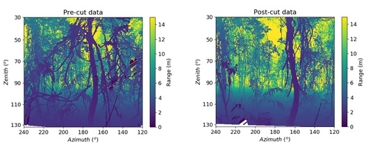
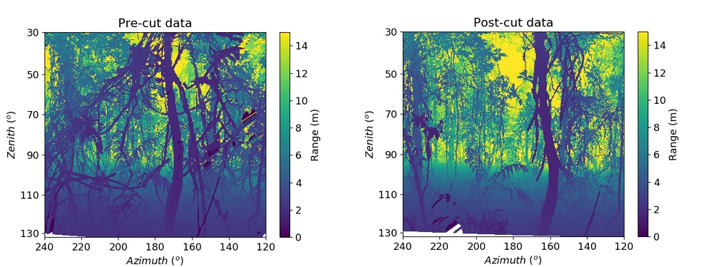
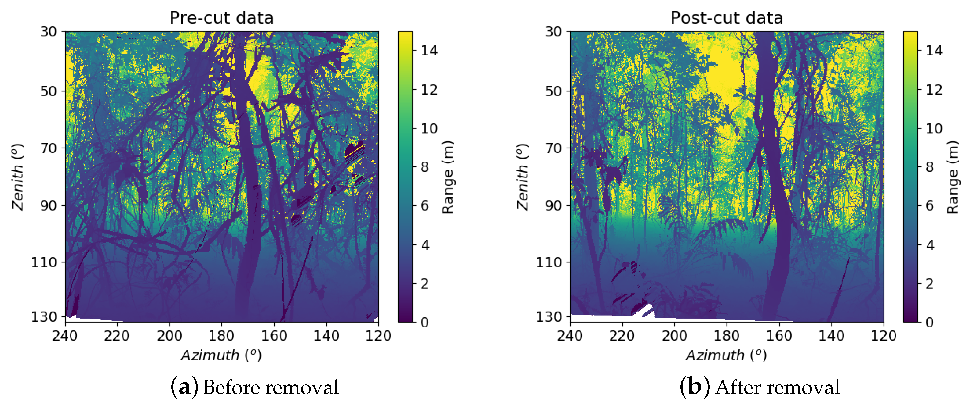
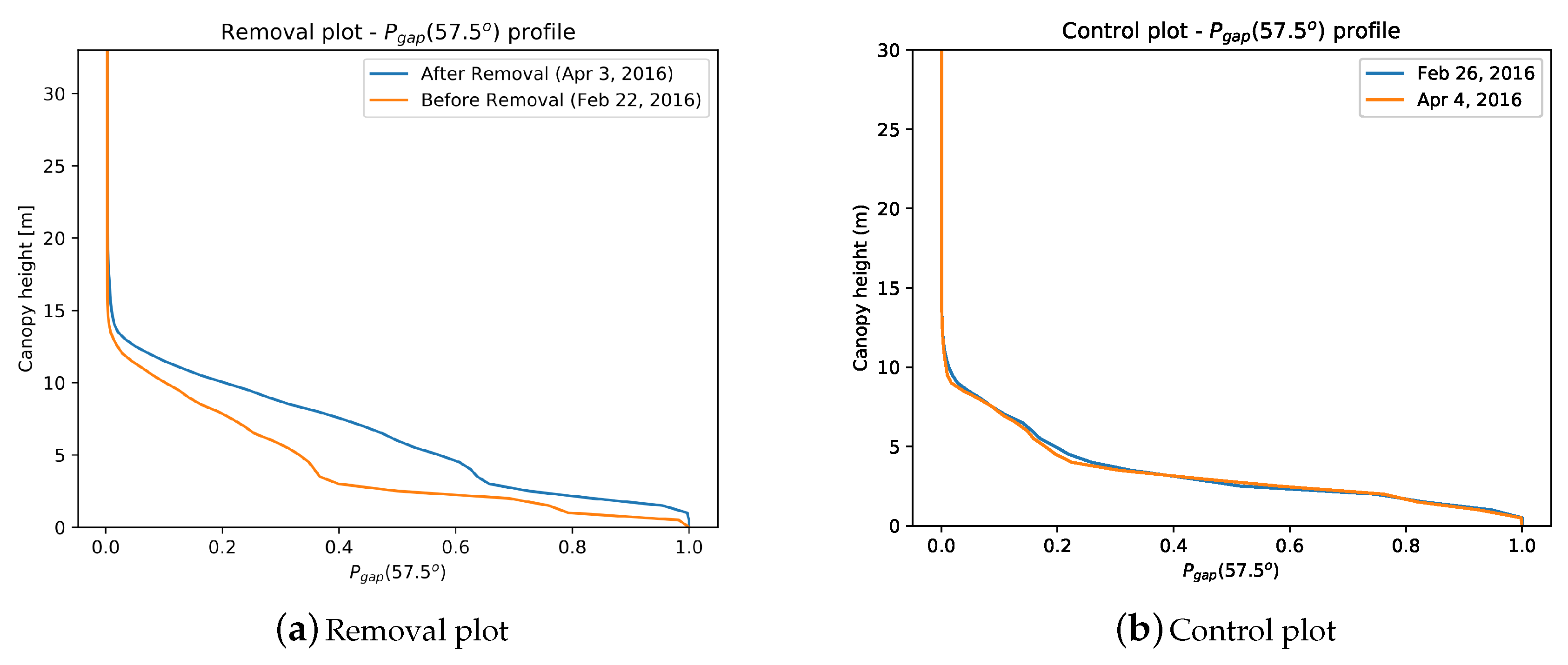
  • to demonstrate the potential of TLS to detect changes in the vertical structure of the forest before and after liana removal
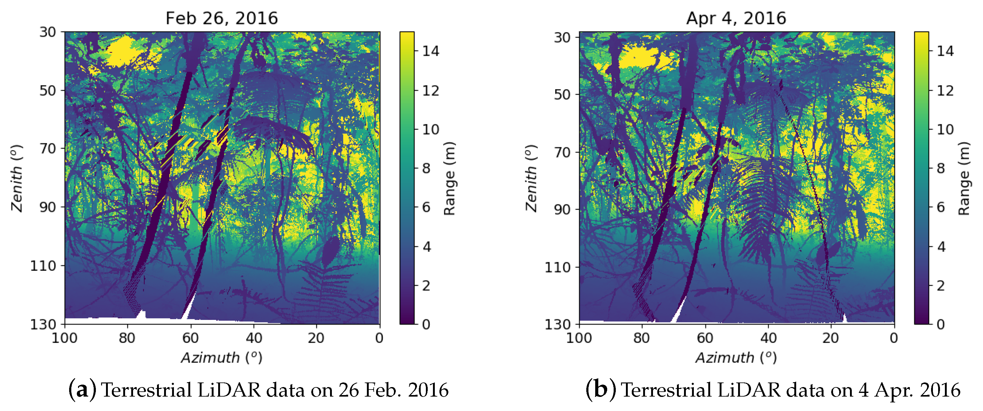
  • to study the reproducibility of the TLS-derived metrics by comparing the structural metrics from two time steps of the control plot.

2. Materials and Methods
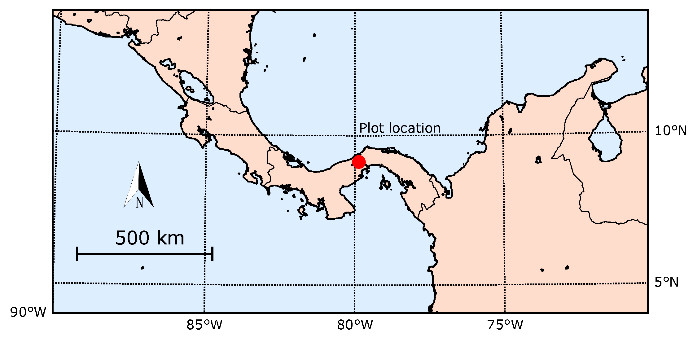
2.1. Study Site

We conducted a liana removal experiment at Gigante Peninsula in Panama (9°9′N, 79°51′W), which is adjacent to Barro Colorado Island (BCI) and is a protected forest part of the Barro Colorado Natural Monument (BCNM). This forest is a 60-year old secondary seasonal tropical forest with recorded average annual rainfall of 2600 mm per year. The site has a distinct dry period for four months from December to April during which the rainfall seldom exceeds 100 mm/month [10,19]. Gigante Peninsula has predominantly clay-rich, highly weathered Oxisols. Tree density and liana density of the site were found to be 3600 stems and 2000 stems ≥1 cm per ha in 2008 [18]. The map of the study site with the control and removal plots marked as red dots is shown in Figure 1.

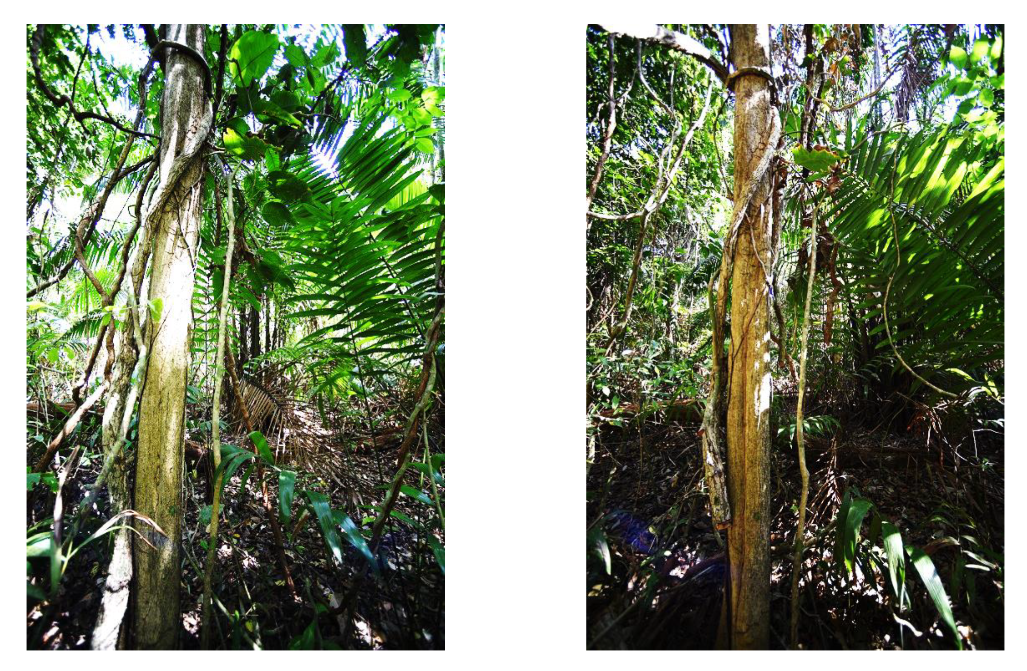
2.2. Experimental Set-Up

We set up two 10 m × 10 m plots, one removal plot and one control plot in February 2016. We measured all trees with diameter ≥10 cm at breast height (1.3 m from ground) and all lianas with diameter ≥1 cm following the liana census protocol in [35] before liana removal. The removal and control plots were approximately 1.5 km far from each other. Since cutting down lianas could release the neighboring trees from below-ground competition, we chose the control plot far from the removal plot [34]. The removal plot had a total of five trees and 66 lianas that were rooted in the plot. Eighteen lianas that were rooted in the plot ascended into the canopy using host trees outside of the 10 m × 10 m plot. We recorded the liana load on trees by counting the number of liana stems that rooted within the plot and attached themselves to the tree trunk or branches in the removal plot. It is possible that some lianas root outside of the plot and go into the canopy of the trees inside the plot. However, it is practically very difficult to follow these lianas as they can root far from the host tree. Hence, only the lianas that root inside the plot are included in the inventory as mentioned in [35]. The control plot had a total of four trees and 45 lianas rooted in the plot. In Table 1, we provide the list of tree diameter, height and liana load of each tree in the removal plot and the tree diameter and height from the control plot. We derived the height of the trees using the region-specific diameter at breast height (DBH) to height allometric equation listed in the study of Van Der Heijden et al. [19]. The height derived from allometric equations do not represent the true height of the trees but rather give an estimate of the tree height.
Trees 2 and 3 were actually the same individual that branched below 1 m from the ground. As a result, we counted the lianas load on one tree also for the other, as it was difficult to distinguish the canopy of these two trees from the ground. Lianas were cut near the forest floor using a machete and most of the liana stems in the understorey were moved without damaging the tree crowns on 23 February 2016 as it can be seen in Figure 2. Lianas in the area of 2 m around the plot were also cut to avoid the edge effects.

2.3. LiDAR Data

We collected TLS data from the two 10 m × 10 m plots, using four scan locations at the corners of the plot. TLS data was collected twice in the removal plot, once on 22 February 2016 one day before liana removal and again on 3 April 2016, six weeks after liana removal, assuming that liana leaves would have mostly fallen off the canopy in the six week time period [6]. We scanned the control plot of size 10 m × 10 m twice with the same time gap of six weeks (26 February 2016–4 April 2016) to account for natural leaf abscission.
We used a RIEGL VZ400 terrestrial laser scanner (RIEGL Laser Measurement Systems GmbH, Horn, Austria), which is a multiple return time-of-flight based scanner using a narrow infrared laser beam of wavelength 1550 nm and a beam divergence of 0.35 mrad. We mounted the scanner on a tripod at approximately 1.3 m from the ground and used an angular sampling resolution of 0.02°. The acquisition time for one full scan with an angular resolution of 0.02° is 12 min 19.6 s. Figure 3 illustrates the view from one scanning position from the removal plot before and after liana removal in a cylindrical projection. Figure 3b of the post-cut TLS data clearly shows the missing liana tangles after liana cutting. Similarly Figure 4 illustrates view from one scanning position for the control plot. As Figure 4b indicates, the TLS data collected on 4 April 2016 indicates displacement of some vegetation such as palm leaves due to wind or arboreal animals.
As the scanner has a zenith range of only 100° from 30° to 130°, to get a full hemispherical view of the canopy, the scanner is tilted to 90° from the vertical axis for an additional tilted scan. We distributed reflective targets in the field to register the upright scan with the corresponding tilt scan and also to co-register all four scan locations. The registration of all four positions for the removal and control plots was done using the RISCAN Pro software (version 2.5.3, RIEGL Laser Measurement Systems GmbH, Horn, Austria) provided by Riegl. After registration, the raw TLS data were exported as ASCII files for deriving CHMs and stem maps. In addition, the raw TLS data were converted into an open source Sorted Pulse Data (SPD) format and analysed using the open source LiDAR data processing library PyLidar for deriving the vertical profiles of Pgap, PAI and PAVD [36,37].

2.4. Co-Registration of Bi-Temporal Data

We co-registered the TLS data before and after liana removal in the removal plot and two scans from the control plot to facilitate the comparison of the all TLS-derived metrics from two different time steps. The point cloud of the region of interest from the two scans of removal and control plot were exported as an ASCII file from RiSCAN pro. The co-registration was done on these ASCII files using an Iterative Closest Point (ICP) algorithm implemented in CloudCompare (version 2.8.1, CloudCompare, GPL software) [38]. The detailed steps of co-registration of the point clouds are described in Appendix A.2. We refer to the normalized z-value as height in this article. Since the topography of the plots studied are relatively flat, we went for a simple plane-fitting normalization as explained in [24].

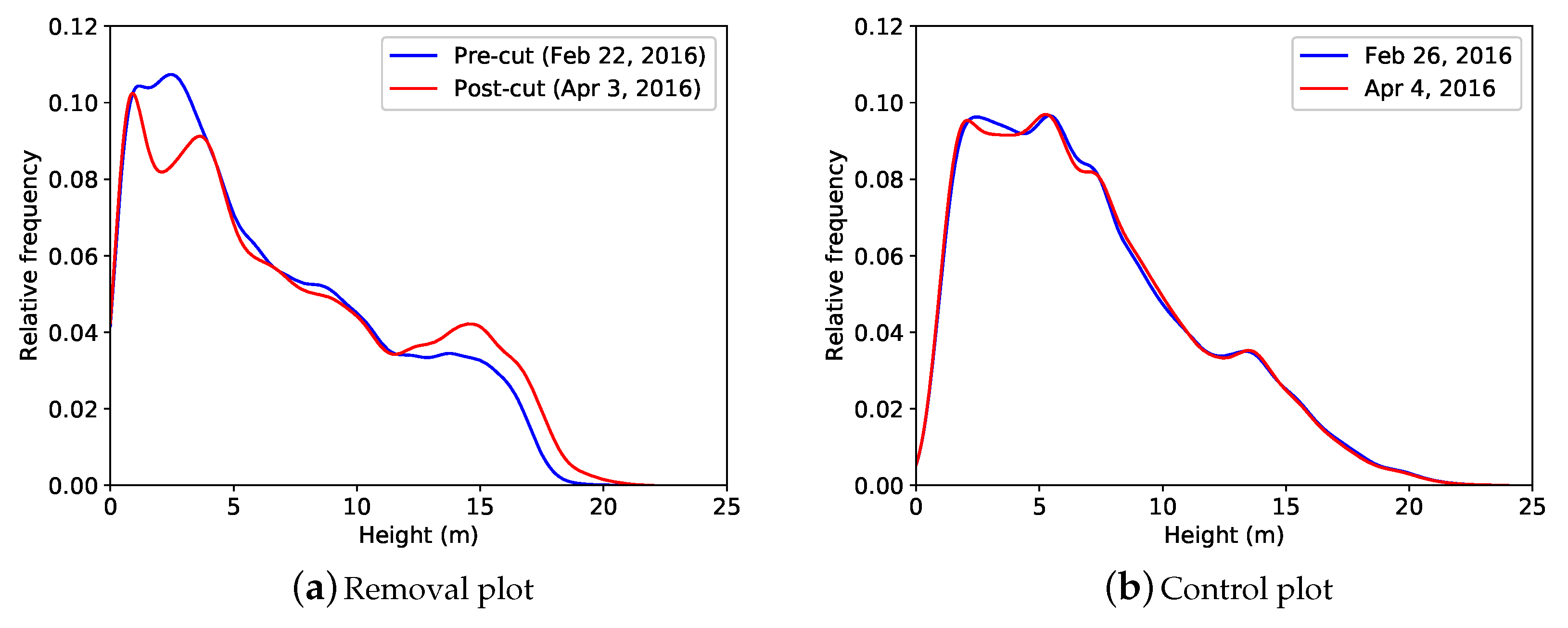
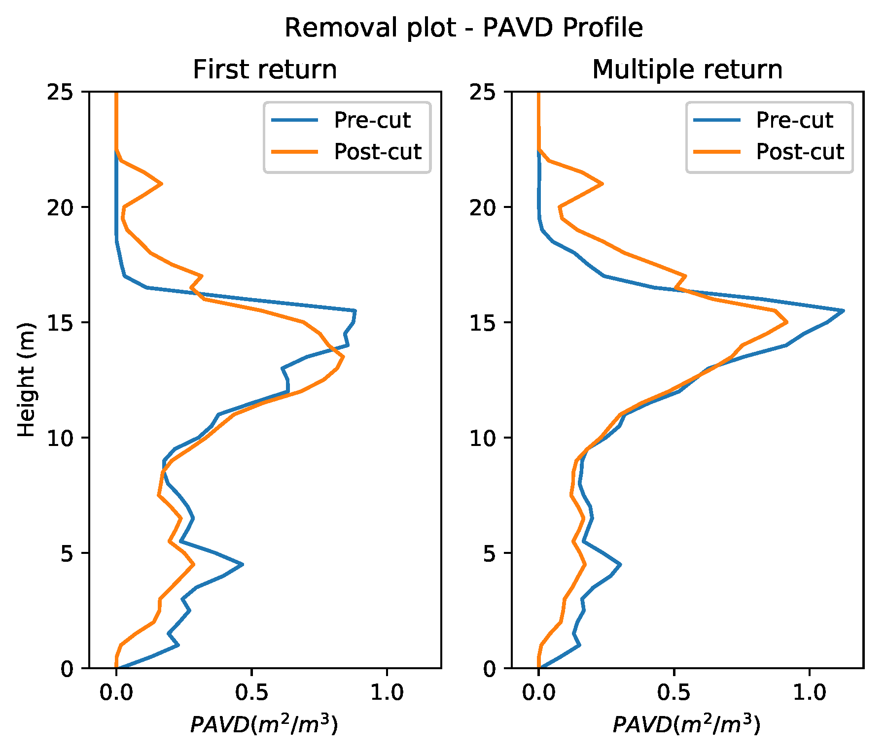
2.5. Vertical Plant Profiles

The frequency distribution of all the returns with respect to height for the bi-temporal data of the removal and the control plot were estimated using a Gaussian kernel density estimator with a bandwidth of 0.5. We also estimated the frequency distribution of the different returns (first, second, third and fourth) with respect to height for the pre- and post-cut data of the removal plot using the kernel density estimator with the same bandwidth of 0.5.
We performed a two-sided Kolmogorov–Smirnov test (KS test) to test the equality of the relative frequency distribution of height of the two time steps for the removal as well as control plot [39]. We chose this test as it does not assume that the data are sampled from a defined distribution like Gaussian distribution.
We described the vertical plant profiles using the vertically resolved gap probability, PAI and PAVD derived from the TLS data. As mentioned in the Section 2.3, we used the open source python library PyLidar for deriving the vertical profiles. We followed the method described in Calders et al. [24] to estimate the Pgap, PAI and PAVD profiles. PAI(z), PAI as a function of height z, is calculated through the estimates of Pgap at the corresponding height. PAVD(z) is calculated based on vertically averaged PAI at 57.5° zenith and Pgap(z). The basic steps and formulas are described in Appendix A.1. For the removal and control plot, we derived the profiles for the specific azimuth region of one scan location shown in Figure 3 and Figure 4, respectively, that fell within the 10 m × 10 m plot. We did not derive the profiles for the data from other scan locations as the scans had many objects too close to the scanner (<1.5 m from the scanner), especially in pre-cut scan, leading to artificial gaps resulting in underestimated PAI.

2.6. Nearest Neighbor Distance

The angular resolution (0.02° in this case) and the range, the distance between the target and the instrument, determine the vertically resolved Average Nearest Neighbor (ANN) distance for the point cloud. The minimum of the average nearest neighbor distance at a particular range is the smallest distance resolvable by the TLS instrument (dmin), which depends on instrument-specific beam divergence [40]. Vertically resolved ANN is calculated as in Equation (1):
ANN ( z ) = 1 N ( z ) i = 1 N ( z ) NN ( p i ) , { p i : z < z p i < z + dz } .
NN is the nearest neighbor distance for a point in the point cloud. The distance between two points in the point cloud for a plot is defined by the Euclidean distance between the two points in 3D. N(z) is the total number of points in the height interval between z and z + dz. For every 1 m z-bin, we calculate the average distance to four nearest neighbors for all the points falling in the bin.
The ANN(z) values indicate the average distance between the topologically connected points from forest floor to canopy. In forests with dense vegetation, ANN(z) is not only influenced by dmin, but also by the spatial distribution of the forest elements occluding the other elements with increasing height [40]. In our study, we compare the ANN(z) between the pre- and post-liana cut TLS data from the removal plot to assess the complex spatial distribution of liana stems and leaves in the plot. We also compare the ANN(z) between the multiple return and the first return TLS data to assess the advantage of using multiple-return scanners over the first-return scanners for studying lianas in the tropics.

2.7. Canopy Height Models

Canopy Height Models describe the horizontal distribution of the height of a forest canopy as a three-dimensional surface [41]. In this study, we generated CHMs to compare the change in height in the observed canopy of the co-registered point clouds in the removal plot before and after liana removal. We also generated CHMs for the two point clouds from the control plot and compare it to that of the removal plot. Bi-temporal TLS data from the removal and control plots were co-registered as described in Appendix A.2. We derived CHMs by selecting the points of highest z-value within each 50 cm × 50 cm x,y grid. After generating CHMs for the two point clouds, we calculated the absolute difference between the corresponding grids of the bi-temporal CHMs to compare the change in the spatial distribution of the observed canopy height for both the removal plot and control plot.

3. Results and Discussion

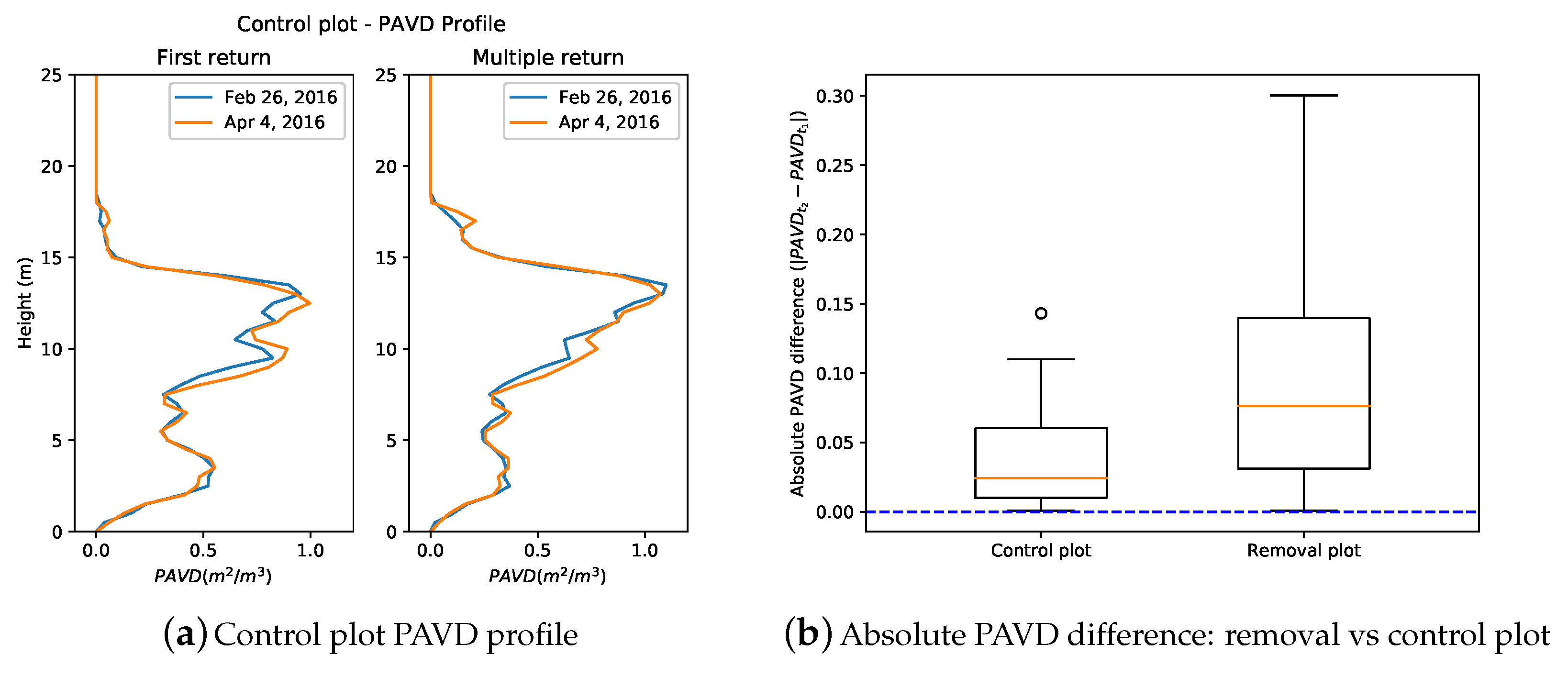
3.1. Vertical Plant Profiles

The frequency distribution of returns with respect to height shows major differences in the number of returns from understorey and the upper canopy of the bi-temporal scans in the removal plot (Figure 5a). After cutting lianas, we found a 10% decrease in the absolute number of returns from the first five meters and a 56% increase in the absolute number of returns above 15 m post liana cutting. The mid-canopy shows very little change before and after liana cutting in terms of the vertical distribution of returns. This is likely because the liana stems in the mid-canopy remained, whereas the liana stems in the understorey were removed while cutting and the liana leaves in the upper canopy had mostly fallen six weeks after liana cutting. In the pre-cut data, there were fewer returns from the upper canopy with lower canopy height compared to the post-cut data because of the occlusion of liana leaves obstructing the pulses emitted.
The pre- and post-cut frequency distributions of height were significantly different in the removal plot (KS statistic = 0.16, P < 0.001), but not in the control plot as it can be seen from Figure 5b (KS statistic = 0.05, P < 0.144).
We found differences in the frequency distribution of height of the different returns in the understorey and the canopy between the pre- and post-cut TLS data (Figure 6). For instance, after liana cutting, the absolute number of returns decreased by 60% in the understorey up to five meters and increased by 70% above 15 m in the post-cut TLS data when only the last returns (fourth return) were considered. Results of the frequency distribution of heights of different returns for the bi-temporal data of the control plot show similar results as in Figure 5b and are therefore not discussed further. However, the results are included in Appendix A.3 for reference.
We derived the vertical profiles of PAVD with both first-return and multiple-return TLS data for the pre- and post-cut scans of the removal plot (Figure 7). The profiles were generated for the azimuth region shown in Figure 3. The total PAI decreased from 6.5 to 6.3 after liana cutting. We found 48% decrease in the first five meters, 18% decrease at 15 m and 90% increase above 16 m in PAVD post-liana cutting when using multiple returns. Both the first return and multiple return PAVD profiles show very little change in the mid-canopy before and after liana cutting similar to the vertical distribution of returns shown in Figure 5a. Both the profiles show increased PAVD beyond 16 m. This increase in PAVD beyond 16 m mainly corresponds to the occlusion of liana leaves in the canopy at about 15 m. Our results demonstrate that liana significantly increases occlusion in the upper canopy owing to their high leaf to stem ratio [5].
Similar to Calders et al. [24], we observed a larger number of laser pulse returns at greater canopy height when using multiple returns as shown in Figure 6 and Figure 7. This highlights the advantage of using a multiple return instrument in forest ecosystems with dense understory and high liana abundance. We recorded 270% more returns from the canopy (≥15 m) when using multiple returns compared to first returns in the pre-cut and post-cut TLS data. In addition, the highest return of pulses for the pre-cut data went down to 18 m from 20 m when only first returns were considered. For the post-cut data, the highest return went down to 19.5 from 22 m. A two meter increase in TLS estimated height post liana cutting clearly indicates that the complex, spatial distribution of different forest elements results in increased occlusion effects with increased height. The height of the largest tree according to region-specific diameter to height allometric equation was 25.19 m and 26.11 m in the removal and control plot, respectively. The maximum height reached by the multiple return TLS used in the study was 22 m (after liana cutting) and 24 m in the removal and control plot, respectively. There are two plausible explanations for this height difference of 3 m in the removal plot and 2 m in the control plot. One possible explanation is that the TLS is underestimating the maximum canopy height owing to tree top occlusions. Tree height measurements from vertex rangefinders have proved to be more accurate in some forest ecosystems compared to TLS and other traditional height measurement methods [42,43,44]. However, this is not always the case as TLS has been proved to reach the top of the canopy easily in other forest ecosystems, where the TLS-derived tree height was compared to true tree height from destructive measurements [45]. The other explanation is that the allometric equation used is overestimating the tree height.
The PAVD profile with only first returns demonstrates more vegetation closer to the scanner in the understory than in the upper canopy compared to the multiple-return PAVD profile. The peak PAVD height before liana cutting remains unchanged at 15.5 m for both first and multiple return profiles. This demonstrates that both the first return and multiple return profiles agree on the height of higher concentration of liana leaves. However, the peak PAVD height after liana cutting went down to 13.5 m from 15 m demonstrating the downside of first return TLS instruments of having a low amount of returns from the canopy despite the mitigated occlusion effects from the loss of other canopy elements.
The bi-temporal vertical profiles of PAVD of the control plot are shown in Figure 8a. Figure 8b shows the box plot of absolute difference between the PAVD of two time steps of the control and removal plot. As it can be seen from Figure 8b, the bi-temporal PAVD profiles of the control plot did not show any major shifts. Our results demonstrate not only the reproducibility of the TLS-derived metrics to do repeated measurements to study the temporal dynamics of tropical forest structure as a function of height, but also the potential of TLS to determine the changes in the vertical profile followed by liana removal. Reproducibility of TLS-derived metrics has also been confirmed in a broadleaf deciduous forest by a spring phenology monitoring study of Calders et al. [27].
We only used one location to derive the vertical profiles of PAVD in the removal plot and control plot. This was mainly because of many objects being close to the scanner (<1.5 m from scanner) especially in the pre-cut scan indicated by the blue zones in Figure 9. Including the blue zones in the zenith band of 55–60° for the estimation of Pgap will result in an overestimated Pgap and thus an underestimated PAI. One way to overcome this is to scan from a location with no interfering vegetation too close to the scanner or to enable the near range activation mode (which is scanner specific, 0.5 m for our instrument). The other way is to correct for these effects using voxel-based methods [46,47], which will be an area of future study.

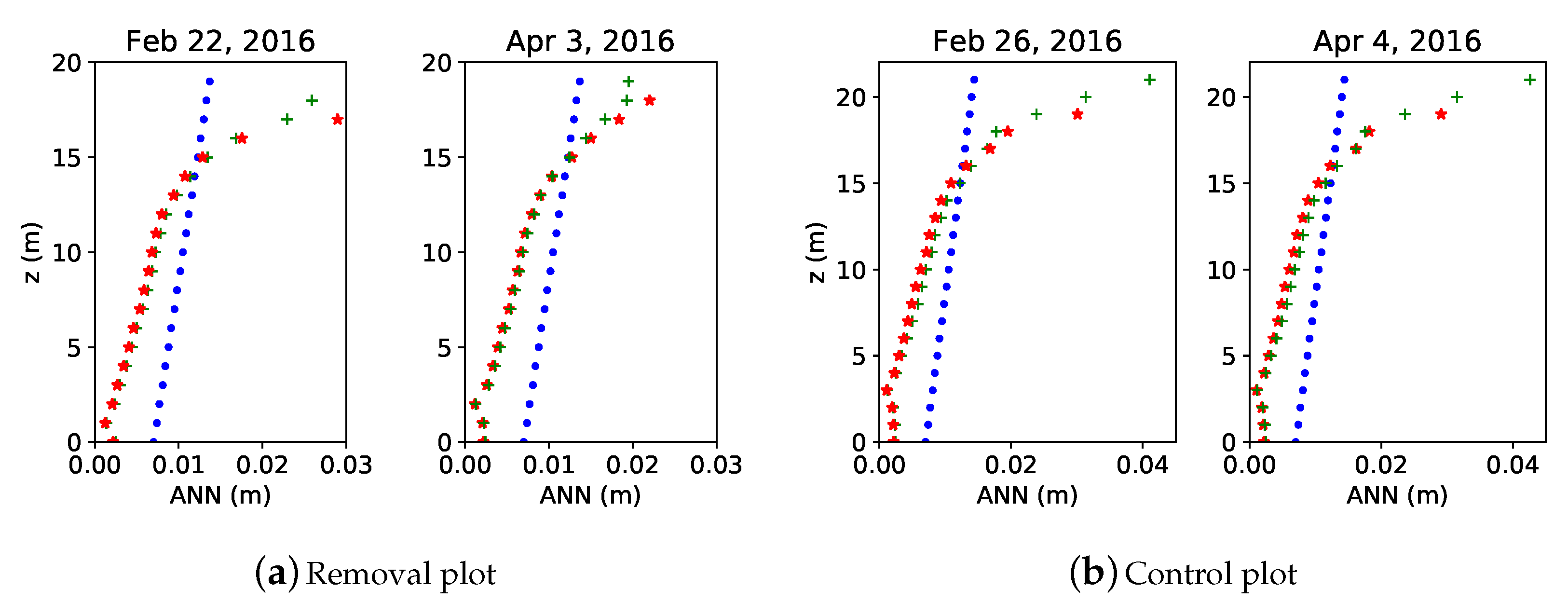
3.2. Nearest Neighbor Distance

Comparison of the multiple-return and the first return ANN (z) for the pre- and post-cut TLS data of the removal plot and the bi-temporal TLS data of the control plot are shown in Figure 10. Lower ANN value for a particular height compared to the corresponding dmin indicates theoretical oversampling and higher ANN value indicates theoretical undersampling. The line representing the laser beam diameter at different heights shows what theoretically can be resolved by the laser beam. The higher the deviation from this line, the higher is the occlusion and lower is the quality of the data.
Pre-cut TLS data clearly shows higher effects of occlusion than the post-cut TLS data in the upper canopy, especially after 15 m. These effects are intensified when using only first returns as the ANN increases by 2 cm from 1 cm and 6 mm from 4 mm between 15 m and 17 m in the pre-cut data and post-cut data, respectively. It is evident from PAVD profiles of Figure 7 that the highest concentration of liana leaves is located at about 15 m leading to an increased ANN above 15 m in the pre-cut data. This implies that, in the first return pre-cut data, the size of the smallest object that could be resolved at 17 m is at least 3 cm and there are not enough topologically connected objects beyond 17 m, whereas with multiple returns the minimum size of the object resolvable at 18 m is 2.5 cm. As this trend is only expected to increase when we move higher up in the canopy, multiple-return TLS has an advantage over first-return TLS to study impact of lianas on forest structure as liana leaves are mainly in the canopy.
Bi-temporal TLS data from the control plot shows no significant difference in the vertical ANN profile. The multiple return ANN at 21 m remains at 4.1 cm and 4.2 cm for the TLS data collected on 26 February 2016 and 4 April 2016, respectively. The same is true for the first return ANN at 19 m, which stays at 3 cm and 2.9 cm for the TLS data on 26 February 2016 and 4 April 2016, respectively. This again demonstrates the potential of TLS to produce reproducible results and to determine the changes in the vertical profile of the forest. However, this also shows the occlusion effects of dense vegetation beyond 15 m, which should be addressed in the upcoming studies focusing on lianas in the tropical biomes.

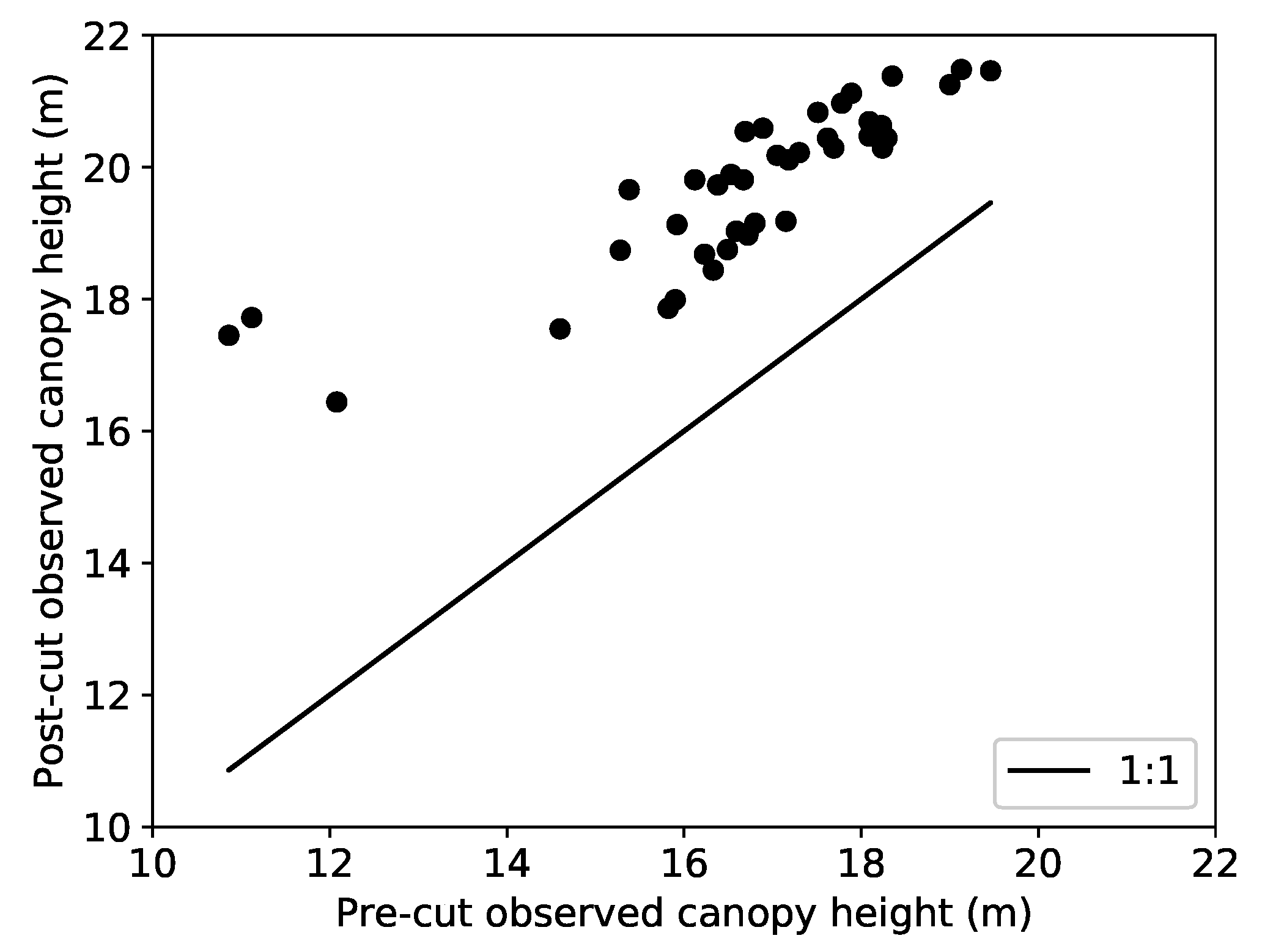
3.3. Canopy Height Models

The difference between the pre- and post-cut CHMs of the removal plot and the bi-temporal scans’ CHMs of the control plot are illustrated in Figure 11. We observed an overall increase in canopy height in the CHM after liana cutting with 82% of the grids seeing an increase in height between 0 to 6 m and 18% of the grids losing vegetation between 0 and 4 m. There were some local changes in the CHM between two time steps in the control plot. The observed increase in canopy height was approximately the same as the observed decrease in the canopy height in the control plot with 54% of the grids of the TLS data from 4 April 2016 gaining height between 0 and 4 m and 46% of the grids losing height between 0 and 4 m. The average observed increase in canopy height was 1.5 m in the removal plot and 0.4 m in the control plot, whereas the average observed height loss was 0.5 m for both the removal and control plot.
It can be seen from Figure 11 that contiguous grids with observed increase in canopy height ranging between 1 and 6 m are co-located with the location of trees 4 and 5 in the removal plot. We interpreted the virtual height gain in these contiguous grids as loss of liana leaves in those grids. Clark and Clark [48] estimated the liana load on trees by two measures: the number of liana stems attached to the tree trunk and Crown Occupancy Index (COI). The COI is estimated on a scale of five based on the percentage of the tree crown occupied by liana leaves (0, 1–25%, 26–50%, 51–75%, 76–100%). They showed that the COI of trees were positively correlated with the basal area of liana load attached to their trunks. We found evidence for their hypothesis as trees 4 and 5 had higher basal area of liana load than the other trees in the plot corresponding to loss of more liana leaves in the canopy. Figure 12 shows the height at which these changes occurred pre- and post-liana cutting in the removal plot. We showed that most of the observed height gain of more than 2 m occur beyond 14 m in the pre-cut data, which is also evident from PAVD profiles in Figure 7. As tree 5 is a small tree with 15.3 cm DBH and 14.9 m height, it is reasonable to assume that most of the height gain occurred within the crown of tree 4, the largest tree of the plot. Our results are in agreement with the other studies, which showed lianas compete more with upper canopy trees for light by colonizing the tree crowns [49,50] and the study of Clark and Clark [48] that showed the liana loads to be positively correlated with tree diameter.
Difference between CHMs of the control plot showed local changes in the canopy. These changes might be either due to the displacement of vegetation or due to loss of some leaves or branches within the six-week period as indicated by Figure 4. However, as Figure 11b,d indicate, the scatterplots confirm the height agreement of bi-temporal data of the control plot as opposed to the bi-temporal data of the removal plot. The TLS instrument used in the study shows the potential for capturing the spatial distribution of changes in the canopy in high detail, which has important implications for the long-term monitoring of liana removal experiments with both removal and control plots [6].

3.4. Limitations of the Study

As explained in the previous sections, occlusion is a challenging problem when deploying TLS in complex environments like tropical forests. The observed increase in canopy height after liana cutting in Figure 11a does not correspond to the real increase in canopy height but rather indicates the occlusion effects of liana leaves in the pre-liana cut CHM. We collected TLS data only from the four corners of the plot. One of the ways to overcome the occlusion is to have a better sampling strategy by increasing the number of scanning locations. Increasing the number of scans around the plot enables us to cover the plot from multiple viewing angles. In addition, scanning the plot from longer distances (approximately 5–10 m from the plot edge) could result in getting better views of the canopy [51]. Our study was able to detect the changes in the vertical structure of the forest, but a better sampling strategy could result in data with better quality enabling the quantification of the changes with higher accuracy. In addition, future development of TLS instruments with smaller beam divergence could help in resolving smaller objects at greater heights in the canopy, thereby mitigating the occlusion effects.
Another important limitation of the study is the plot size and sample size. We used a small sample size because our study is a first exploratory effort to test the potential of TLS to study the effect of lianas on forest structure. We tried to balance the number of lianas that we sacrificed for this study by cutting enough lianas to rigorously see the effect of liana cutting on forest structure, but not so many that it would have a huge impact on natural forest regeneration and functioning. Though our study cannot conclude about the ecological impact of lianas on forest structure, the changes observed in the PAVD profiles, ANN(z) profiles and the CHMs of the removal plot derived from the TLS data have important implications for the future studies of liana impact on the forest structure. Collecting high quality TLS data for large areas in dense forest ecosystems can be time-consuming. For instance, scanning a 1 ha plot with scan positions located every 10 m and few scan positions located outside of the plot boundaries in a dense tropical forest could take up to five days including the time taken for preparing the plot (distributing the control reflective targets for registration). However, such high detailed data can yield answers to some of the unsolved ecological questions about liana influence on forest structure.

4. Conclusions

As lianas strongly compete with trees for light, studying the changes in the vertical forest structure with and without lianas over the long term could explain how lianas impact the forest structure. We demonstrate the potential of TLS to study the changes in all the vertical strata of the forest caused by liana removal. Our results demonstrate the advantages of having multiple returns over first returns to quantify changes in the upper canopy of the forest, especially in environments where the understorey is dense or lianas are abundant. Our results also highlight the reproducibility of TLS derived metrics to do repeated long-term measurements of the liana removal and control plots. Though collecting TLS data from large areas in complex environments can be time-consuming, lessons learned from the current small scale study will enable us to collect high quality data in future. We highly recommend to include TLS observations in future large scale liana removal experiments in the long term to quantitatively study the impact of lianas on the forest structure.

Author Contributions

S.M.K.M., M.d.P.e.B., S.S. and H.V. conceived and designed the experiments; S.M.K.M., M.d.P.e.B. and S.S. performed the experiments; S.M.K.M. and K.C. analyzed the data; S.M.K.M., K.C., and H.V. wrote the paper. All authors discussed the results and commented on the manuscript.

Acknowledgments

The research leading to these results was funded by the European Research Council Starting Grant 637643 (TREECLIMBERS) and National Science Foundation grants: NSF-IOS 1558093 and NSF-DEB 1822473. We thank Iebe Stroobants, Elizabeth Kearsley, Maria M. García León, Felipe Nery Arantes Mello, Claudio Manuel Monteza and Patrick Cvecko for their assistance with fieldwork. The authors would like to thank the Smithsonian Tropical Research Institute (STRI) for their support and for allowing us to perform liana removal experiments in Gigante.

Conflicts of Interest

The authors declare no conflict of interest.

Abbreviations

The following abbreviations are used in this manuscript:
TLSTerrestrial Laser Scanning
DBHDiameter at Breast Height
PAIPlant Area Index
LAILeaf Area Index
PAVDPlant Area Volume Density
CHMCanopy Height Model
LiDARLight Detection and Ranging
PCLPortable Canopy LiDAR
COICrown Occupancy Index
BCIBarro Colorado Island
BCNMBarro Colorado Natural Monunment
SPDSorted Pulse Data
ICPIterative Closest Point
KSKolmogorov–Smirnov
ANNAverage Nearest Neighbor

Appendix A

Appendix A.1. Vertical Profiles of Pgap, PAI and PAVD

The basic steps and formulas for deriving the vertical profiles of Pgap, PAI and PAVD based on Calders et al. [24] are described in this section.
Pgap (z) from a multi-return LiDAR is estimated using Equation (A1):
Pgap ( θ ¯ , z ) = 1 w i ( z i z , θ ¯ ) N ( θ ¯ ) , w = 1 n s .
z is the height above ground. θ ¯ is the mid-point of the finite zenith angle interval used to aggregate the gap probability at a certain height z. N( θ ¯ ) is the total number of laser pulses sent for the zenith angle interval and n s is the total number of returns for that transmitted pulse. In this study, we used the zenith angle between 5° and 60° and a zenith angle interval of 5 degrees. We only used a 90° azimuth for every scan position that fell within the 10 m × 10 m plot area.
PAI (z) and total PAI are calculated as in Equations (A2) and (A3), respectively:
PAI ( z ) = 1.1 log Pgap ( 57.5 , z ) ,
PAI = PAI ( H ) .
H is the canopy height. PAI is calculated at the hinge region (57.5°), by using the laser pulses transmitted and reflected within the zenith band of 55° and 60°. The hinge region is used mainly because the foliage distribution function is assumed to be invariant in this region.
PAVD(z) is calculated using the PAI at the hinge region and the Pgap(z) based on Equation (A4) described in Jupp et al. [23]:
PAVD ( z ) = PAI δ δ z log Pgap ( θ ¯ , z ) log Pgap ( θ ¯ , H ) .
In addition to restricting the pulses transmitted and reflected within a specific azimuth falling within the area of the plot, we also excluded those azimuth angle intervals from the scans that had no returns registered because an object was too close to the scanner (within 1.5 m from the scanner).
Vertical profiles of Pgap derived for the hinge region between 55° and 60° for the pre-cut and post-cut scans of the removal plot and the bi-temporal scans of the control plot are shown in Figure A1a,b, respectively.
Figure A1. Pgap profile in the hinge region (57.5° zenith).
Remotesensing 10 00810 g0a1

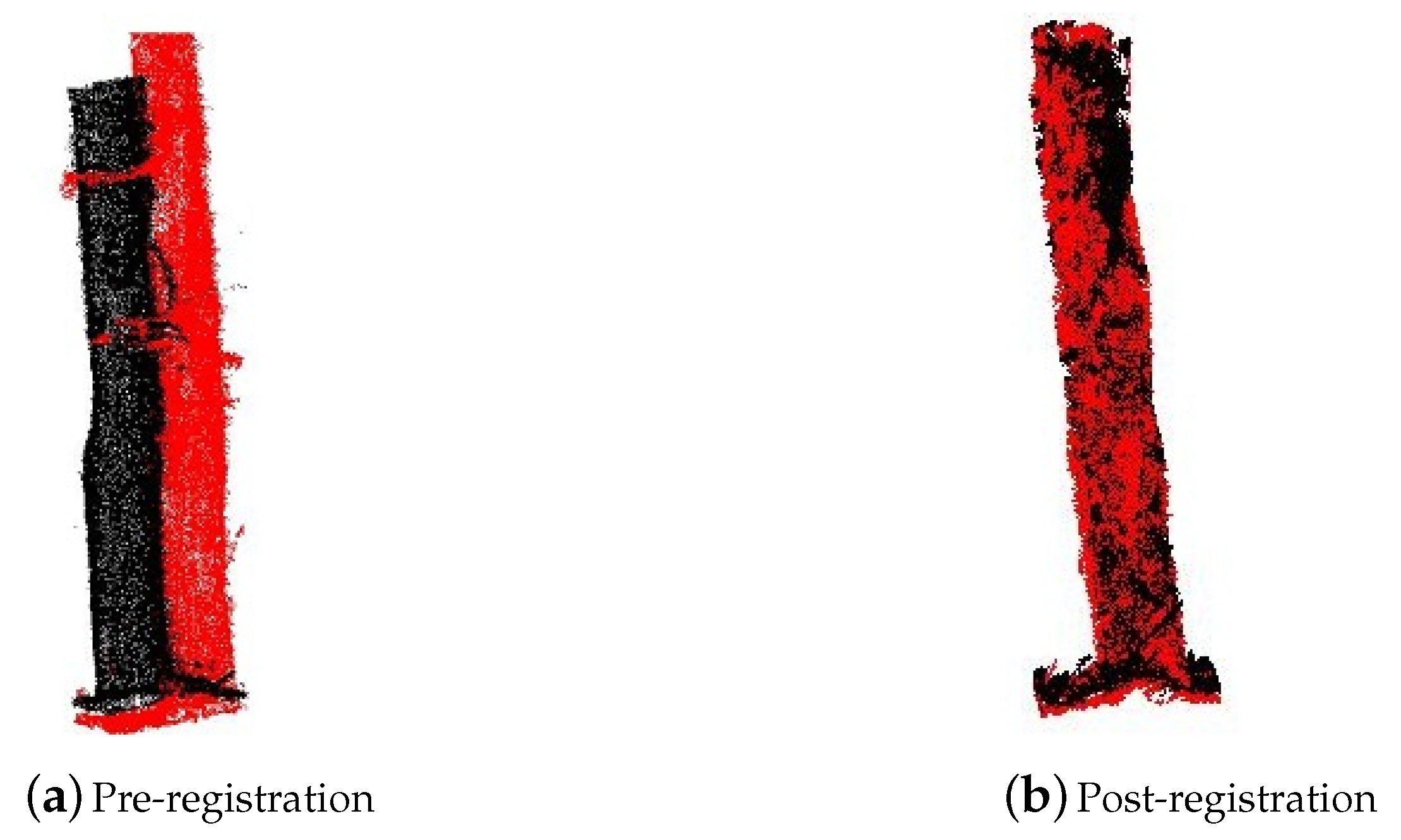
Appendix A.2. Co-Registration of the Bi-Temporal Scans

Co-registration was done as follows:
  • We isolated the ground points from the TLS data of two time steps for both the removal and control plot using the Cloth Simulation Filter (CSF) algorithm implemented in CloudCompare. CSF is a tool to extract ground points from a discrete return LiDAR data [52].
  • We derived stem maps from TLS for the two time steps following the method mentioned in Section 2.7.
  • We used the stem points plus the ground points from these two pieces of different temporal data as input for the first coarse manual registration in CloudCompare with one point cloud as reference and the other as the one to be aligned.
  • We then applied the transformation matrix from the manual registration to the whole point cloud to be aligned.
  • We used the ICP algorithm [53] implemented in CloudCompare for fine registration after the first coarse manual registration. We selected all the points from the ground up to 4 m for fine registration.
  • We applied the transformation matrix that resulted from the ICP fine registration to the whole point cloud to be aligned.
Co-registration of the bi-temporal TLS data was achieved with an RMSE of 0.08 m in the removal plot and 0.06 m in the control plot, respectively. Figure A2 shows the result of co-registration using a tree trunk from the removal plot.
Figure A2. Illustration of co-registration using a tree trunk from the removal plot. Black: Pre-cut data and Red: Post-cut data.
Remotesensing 10 00810 g0a2

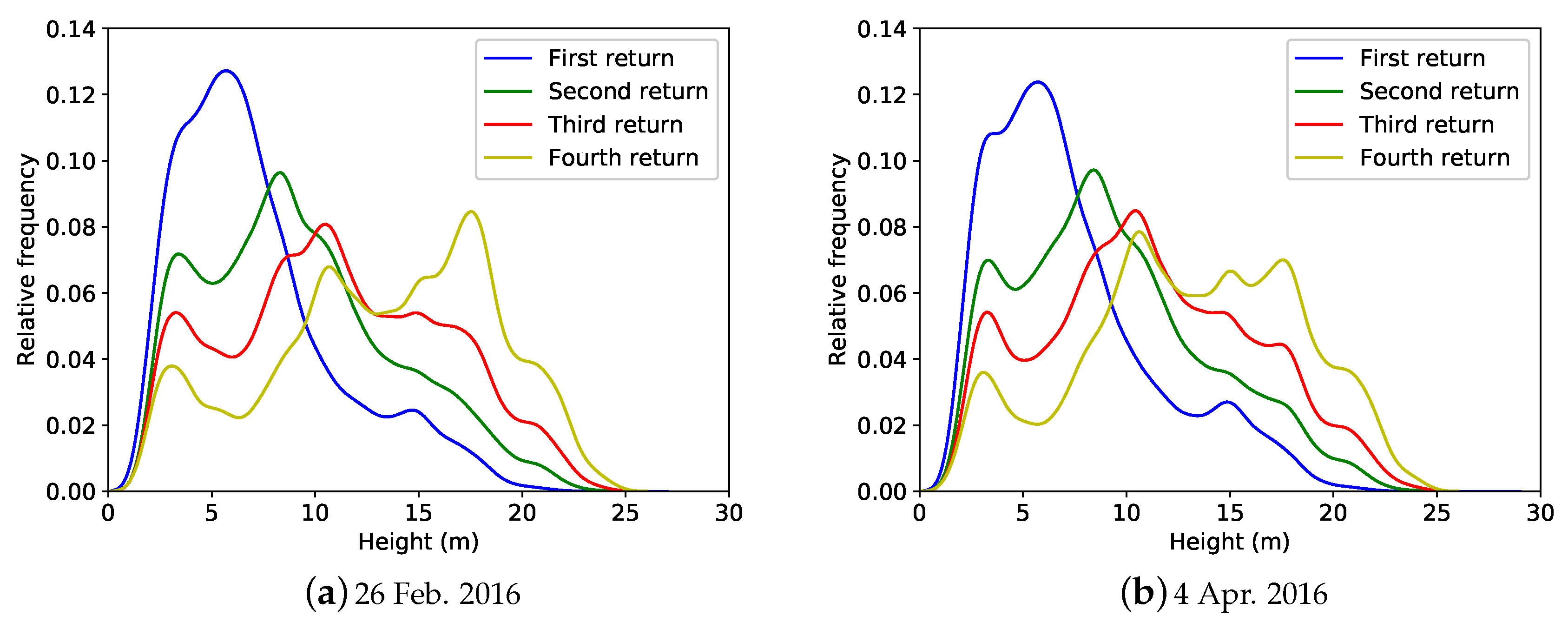
Appendix A.3. Additional Results

Result of the frequency distribution of height of different returns for the bi-temporal data of the control plot, which shows similar results as in Figure 5b, is shown in Figure A3.
Figure A3. Comparison of the frequency distribution with Gaussian kernel density estimation of different vertical returns with height between 26 February 2016 (a) and 4 April 2016 (b) data of the control plot.
Remotesensing 10 00810 g0a3

References

  1. Crowley, T.J. Causes of climate change over the past 1000 years. Science 2000, 289, 270–277. [Google Scholar] [CrossRef] [PubMed]
  2. Woods, P. Effects of logging, drought, and fire on structure and composition of tropical forests in Sabah, Malaysia. Biotropica 1989, 21, 290–298. [Google Scholar] [CrossRef]
  3. Wright, S.J. Tropical forests in a changing environment. Trends Ecol. Evol. 2005, 20, 553–560. [Google Scholar] [CrossRef] [PubMed]
  4. Schnitzer, S.A.; Bongers, F. Increasing liana abundance and biomass in tropical forests: Emerging patterns and putative mechanisms. Ecol. Lett. 2011, 14, 397–406. [Google Scholar] [CrossRef] [PubMed]
  5. Schnitzer, S.A.; Bongers, F. The ecology of lianas and their role in forests. Trends Ecol. Evol. 2002, 17, 223–230. [Google Scholar] [CrossRef]
  6. Rodríguez-Ronderos, M.E.; Bohrer, G.; Sanchez-Azofeifa, A.; Powers, J.S.; Schnitzer, S.A. Contribution of lianas to plant area index and canopy structure in a Panamanian forest. Ecology 2016, 97, 3271–3277. [Google Scholar] [CrossRef] [PubMed]
  7. Muthumperumal, C.; Parthasarathy, N. Diversity, distribution and resource values of woody climbers in tropical forests of southern Eastern Ghats, India. J. For. Res. 2013, 24, 365–374. [Google Scholar] [CrossRef]
  8. Bongers, F.; Schnitzer, S.; Traore, D. The importance of lianas and consequences for forest management in West Africa. BioTerre. 2002. Available online: https://www.researchgate.net/profile/Frans_Bongers/publication/40797530_The_importance_of_lianas_and_consequences_for_forest_management_in_West_Africa/links/0c960529614f4e6557000000.pdf (accessed on 22 March 2018).
  9. Hegarty, E.E. Distribution and abundance of vines in forest communities. Biol. Vines 1991, 313–334. [Google Scholar]
  10. Schnitzer, S.A.; Carson, W.P. Treefall gaps and the maintenance of species diversity in a tropical forest. Ecology 2001, 82, 913–919. [Google Scholar] [CrossRef]
  11. Vidal, E.; Johns, J.; Gerwing, J.J.; Barreto, P.; Uhl, C. Vine management for reduced-impact logging in eastern Amazonia. For. Ecol. Manag. 1997, 98, 105–114. [Google Scholar] [CrossRef]
  12. Putz, F.E. The natural history of lianas on Barro Colorado Island, Panama. Ecology 1984, 65, 1713–1724. [Google Scholar] [CrossRef]
  13. Appanah, S.; Putz, F. Climber abundance in virgin dipterocarp forest and the effect of pre-felling climber cutting on logging damage [Peninsular Malaysia]. Malays. For. 1984, 47, 335–342. [Google Scholar]
  14. Schnitzer, S.A.; Parren, M.P.; Bongers, F. Recruitment of lianas into logging gaps and the effects of pre-harvest climber cutting in a lowland forest in Cameroon. For. Ecol. Manag. 2004, 190, 87–98. [Google Scholar] [CrossRef]
  15. Pérez-Salicrup, D.R. Effect of liana cutting on tree regeneration in a liana forest in Amazonian Bolivia. Ecology 2001, 82, 389–396. [Google Scholar] [CrossRef]
  16. Gerwing, J.J. Testing liana cutting and controlled burning as silvicultural treatments for a logged forest in the eastern Amazon. J. Appl. Ecol. 2001, 38, 1264–1276. [Google Scholar] [CrossRef]
  17. Marshall, A.R.; Coates, M.A.; Archer, J.; Kivambe, E.; Mnendendo, H.; Mtoka, S.; Mwakisoma, R.; Figueiredo, R.J.; Njilima, F.M. Liana cutting for restoring tropical forests: A rare palaeotropical trial. Afr. J. Ecol. 2017, 55, 282–297. [Google Scholar] [CrossRef] [Green Version]
  18. Reid, J.P.; Schnitzer, S.A.; Powers, J.S. Short and long-term soil moisture effects of liana removal in a seasonally moist tropical forest. PLoS ONE 2015, 10, e0141891. [Google Scholar] [CrossRef] [PubMed]
  19. Van Der Heijden, G.M.; Powers, J.S.; Schnitzer, S.A. Lianas reduce carbon accumulation and storage in tropical forests. Proc. Natl. Acad. Sci. USA 2015, 112, 13267–13271. [Google Scholar] [CrossRef] [PubMed]
  20. Hancock, S.; Essery, R.; Reid, T.; Carle, J.; Baxter, R.; Rutter, N.; Huntley, B. Characterising forest gap fraction with terrestrial lidar and photography: An examination of relative limitations. Agric. For. Meteorol. 2014, 189, 105–114. [Google Scholar] [CrossRef] [Green Version]
  21. Calders, K.; Origo, N.; Disney, M.; Nightingale, J.; Woodgate, W.; Armston, J.; Lewis, P. Variability and bias in active and passive ground-based measurements of effective plant, wood and leaf area index. Agric. For. Meteorol. 2018, 252, 231–240. [Google Scholar] [CrossRef]
  22. Danson, F.M.; Hetherington, D.; Morsdorf, F.; Koetz, B.; Allgower, B. Forest canopy gap fraction from terrestrial laser scanning. IEEE Geosci. Remote Sens. Lett. 2007, 4, 157–160. [Google Scholar] [CrossRef] [Green Version]
  23. Jupp, D.L.; Culvenor, D.; Lovell, J.; Newnham, G.; Strahler, A.; Woodcock, C. Estimating forest LAI profiles and structural parameters using a ground-based laser called ‘Echidna®. Tree Physiol. 2009, 29, 171–181. [Google Scholar] [CrossRef] [PubMed]
  24. Calders, K.; Armston, J.; Newnham, G.; Herold, M.; Goodwin, N. Implications of sensor configuration and topography on vertical plant profiles derived from terrestrial LiDAR. Agric. For. Meteorol. 2014, 194, 104–117. [Google Scholar] [CrossRef]
  25. Yang, X.; Strahler, A.H.; Schaaf, C.B.; Jupp, D.L.; Yao, T.; Zhao, F.; Wang, Z.; Culvenor, D.S.; Newnham, G.J.; Lovell, J.L.; et al. Three-dimensional forest reconstruction and structural parameter retrievals using a terrestrial full-waveform lidar instrument (Echidna®). Remote Sens. Environ. 2013, 135, 36–51. [Google Scholar] [CrossRef]
  26. Liang, X.; Litkey, P.; Hyyppa, J.; Kaartinen, H.; Vastaranta, M.; Holopainen, M. Automatic stem mapping using single-scan terrestrial laser scanning. IEEE Trans. Geosci. Remote Sens. 2012, 50, 661–670. [Google Scholar] [CrossRef]
  27. Calders, K.; Schenkels, T.; Bartholomeus, H.; Armston, J.; Verbesselt, J.; Herold, M. Monitoring spring phenology with high temporal resolution terrestrial LiDAR measurements. Agric. For. Meteorol. 2015, 203, 158–168. [Google Scholar] [CrossRef]
  28. Srinivasan, S.; Popescu, S.C.; Eriksson, M.; Sheridan, R.D.; Ku, N.W. Multi-temporal terrestrial laser scanning for modeling tree biomass change. For. Ecol. Manag. 2014, 318, 304–317. [Google Scholar] [CrossRef]
  29. Liang, X.; Hyyppä, J.; Kaartinen, H.; Holopainen, M.; Melkas, T. Detecting changes in forest structure over time with bi-temporal terrestrial laser scanning data. ISPRS Int. J. Geo-Inf. 2012, 1, 242–255. [Google Scholar] [CrossRef]
  30. Olivier, M.D.; Robert, S.; Fournier, R.A. A method to quantify canopy changes using multi-temporal terrestrial lidar data: Tree response to surrounding gaps. Agric. For. Meteorol. 2017, 237, 184–195. [Google Scholar] [CrossRef]
  31. Parker, G.G.; Harding, D.J.; Berger, M.L. A portable LIDAR system for rapid determination of forest canopy structure. J. Appl. Ecol. 2004, 41, 755–767. [Google Scholar] [CrossRef]
  32. Sánchez-Azofeifa, A.; Portillo-Quintero, C.; Durán, S. Structural effects of liana presence in secondary tropical dry forests using ground LiDAR. Biogeosci. Discuss. 2015, 12, 17153–17175. [Google Scholar] [CrossRef]
  33. Sánchez-Azofeifa, G.A.; Guzmán-Quesada, J.A.; Vega-Araya, M.; Campos-Vargas, C.; Durán, S.M.; D’Souza, N.; Gianoli, T.; Portillo-Quintero, C.; Sharp, I. Can terrestrial laser scanners (TLSs) and hemispherical photographs predict tropical dry forest succession with liana abundance? Biogeosciences 2017, 14, 977. [Google Scholar] [CrossRef]
  34. Schnitzer, S.A.; Kuzee, M.E.; Bongers, F. Disentangling above-and below-ground competition between lianas and trees in a tropical forest. J. Ecol. 2005, 93, 1115–1125. [Google Scholar] [CrossRef]
  35. Schnitzer, S.A.; Rutishauser, S.; Aguilar, S. Supplemental protocol for liana censuses. For. Ecol. Manag. 2008, 255, 1044–1049. [Google Scholar] [CrossRef]
  36. Bunting, P.; Armston, J.; Lucas, R.M.; Clewley, D. Sorted pulse data (SPD) library. Part I: A generic file format for LiDAR data from pulsed laser systems in terrestrial environments. Comput. Geosci. 2013, 56, 197–206. [Google Scholar] [CrossRef]
  37. Bunting, P.; Armston, J.; Clewley, D.; Lucas, R.M. Sorted pulse data (SPD) library—Part II: A processing framework for LiDAR data from pulsed laser systems in terrestrial environments. Comput. Geosci. 2013, 56, 207–215. [Google Scholar] [CrossRef]
  38. Girardeau-Montaut, D. Cloudcompare-Open Source Project. OpenSource Project. 2011. Available online: http://www.danielgm.net/cc/ (accessed on 14 November 2016).
  39. Massey, F.J., Jr. The Kolmogorov-Smirnov test for goodness of fit. J. Am. Stat. Assoc. 1951, 46, 68–78. [Google Scholar] [CrossRef]
  40. Burt, A.; Disney, M.; Calders, K. Extracting individual trees from lidar point clouds using treeseg. Methods Ecol. Evol. 2018. in review. [Google Scholar]
  41. Popescu, S.C.; Wynne, R.H.; Nelson, R.F. Measuring individual tree crown diameter with lidar and assessing its influence on estimating forest volume and biomass. Can. J. Remote Sens. 2003, 29, 564–577. [Google Scholar] [CrossRef]
  42. Krooks, A.; Kaasalainen, S.; Kankare, V.; Joensuu, M.; Raumonen, P.; Kaasalainen, M. Predicting tree structure from tree height using terrestrial laser scanning and quantitative structure models. Silva Fenn 2014, 48, 1125. [Google Scholar] [CrossRef]
  43. Larjavaara, M.; Muller-Landau, H.C. Measuring tree height: A quantitative comparison of two common field methods in a moist tropical forest. Methods Ecol. Evol. 2013, 4, 793–801. [Google Scholar] [CrossRef]
  44. Maas, H.G.; Bienert, A.; Scheller, S.; Keane, E. Automatic forest inventory parameter determination from terrestrial laser scanner data. Int. J. Remote Sens. 2008, 29, 1579–1593. [Google Scholar] [CrossRef]
  45. Calders, K.; Newnham, G.; Burt, A.; Murphy, S.; Raumonen, P.; Herold, M.; Culvenor, D.; Avitabile, V.; Disney, M.; Armston, J.; et al. Nondestructive estimates of above-ground biomass using terrestrial laser scanning. Methods Ecol. Evol. 2015, 6, 198–208. [Google Scholar] [CrossRef]
  46. Fournier, R.A.; Côté, J.F.; Bourge, F.; Durrieu, S.; Piboule, A.; Béland, M. A method addressing signal occlusion by scene objects to quantify the 3D distribution of forest components from terrestrial lidar. In Proceedings of the SilviLaser 2015, La Grande Motte, France, 28–30 September 2015; pp. 29–31. [Google Scholar]
  47. Hancock, S.; Anderson, K.; Disney, M.; Gaston, K.J. Measurement of fine-spatial-resolution 3D vegetation structure with airborne waveform lidar: Calibration and validation with voxelised terrestrial lidar. Remote Sens. Environ. 2017, 188, 37–50. [Google Scholar] [CrossRef]
  48. Clark, D.B.; Clark, D.A. Distribution and effects on tree growth of lianas and woody hemiepiphytes in a Costa Rican tropical wet forest. J. Trop. Ecol. 1990, 6, 321–331. [Google Scholar] [CrossRef]
  49. Avalos, G.; Mulkey, S.S.; Kitajima, K.; Wright, S.J. Colonization strategies of two liana species in a tropical dry forest canopy. Biotropica 2007, 39, 393–399. [Google Scholar] [CrossRef]
  50. Tobin, M.F.; Wright, A.J.; Mangan, S.A.; Schnitzer, S.A. Lianas have a greater competitive effect than trees of similar biomass on tropical canopy trees. Ecosphere 2012, 3, 1–11. [Google Scholar] [CrossRef]
  51. Wilkes, P.; Lau, A.; Disney, M.; Calders, K.; Burt, A.; de Tanago, J.G.; Bartholomeus, H.; Brede, B.; Herold, M. Data acquisition considerations for Terrestrial Laser Scanning of forest plots. Remote Sens. Environ. 2017, 196, 140–153. [Google Scholar] [CrossRef]
  52. Zhang, W.; Qi, J.; Wan, P.; Wang, H.; Xie, D.; Wang, X.; Yan, G. An easy-to-use airborne LiDAR data filtering method based on cloth simulation. Remote Sens. 2016, 8, 501. [Google Scholar] [CrossRef]
  53. Besl, P.J.; McKay, N.D. Method for registration of 3-D shapes. In Sensor Fusion IV: Control Paradigms and Data Structures; International Society for Optics and Photonics: Bellingham, WA, USA, 1992; Volume 1611, pp. 586–607. [Google Scholar]
Figure 1. Map of the study site with the location of the removal and control plots marked with the red dot. The study site is located in Gigante Peninsula in Panama (9°9′N, 79°51′W) adjacent to Barro Colorado Island (BCI).
Remotesensing 10 00810 g001
Figure 2. Comparison of the removal plot before (left) and after (right) liana removal.
Remotesensing 10 00810 g002
Figure 3. View of terrestrial LiDAR data from one scan position of the removal plot with azimuth ranging from 120° to 240° and zenith ranging from 30° to 130°. The data is colored according to the range of the laser pulse.
Remotesensing 10 00810 g003
Figure 4. View of terrestrial LiDAR data from one scan position of the control plot with azimuth ranging from 0° to 100° and zenith ranging from 30° to 130°. The data is colored according to the range of the laser pulse.
Remotesensing 10 00810 g004
Figure 5. Comparison of frequency distribution with Gaussian kernel density estimation of all vertical returns combined for the bi-temporal TLS data from the removal (a) and control plot (b).
Remotesensing 10 00810 g005
Figure 6. Comparison of the frequency distribution with Gaussian kernel density estimation of different vertical returns with height between the pre-cut (a) and post-cut (b) data of the removal plot.
Remotesensing 10 00810 g006
Figure 7. Comparison of the first-return and multiple-return Plant Area Volume Density (PAVD) profiles of the removal plot.
Remotesensing 10 00810 g007
Figure 8. (a) shows the bi-temporal Plant Area Volume Density (PAVD) profiles of the control plot and (b) shows the absolute PAVD difference box plot of the control and removal plot, with t2 being the data from second time step and t1, the first time step.
Remotesensing 10 00810 g008
Figure 9. TLS data before liana removal with azimuth ranging from 0° to 360° and zenith ranging from 30° to 130°. The data is colored according to range of the laser pulse with black being low and white being high. The areas with blue indicates regions of no returns either because the object was too close to the scanner (<1.5 m) or because of a gap.
Remotesensing 10 00810 g009
Figure 10. Comparison of multiple return vs. first return vertically resolved average nearest neighbor distance (ANN(z)) for pre- and post-cut TLS data of the removal plot (a) and bi-temporal data of the control plot (b). ( Laser beam diameter, First return and + Multiple return).
Remotesensing 10 00810 g010
Figure 11. Difference map of the Canopy Height Models (CHM) with circles representing the location of trees ≥10 cm in DBH. (a) removal plot and (c) control plot. The size of the circles correspond to the size of the trees. The color scale represents the change in height in meters between the two time steps. Scatter plot showing the CHM difference between bi-temporal TLS data for removal plot (b) and control plot (d).
Remotesensing 10 00810 g011
Figure 12. Differences in Canopy Height Models (CHM) for CHMpost-cut − CHMpre-cut ≥ 2 m in the removal plot.
Remotesensing 10 00810 g012
Table 1. Overview of trees, diameter and number of liana stems on each trees in the removal and control plot. Trees 2 and 3 are the same individual that branched below 1 m from the ground.
Plot TypeTree No.Diameter at
Breast Height (cm)
Height (m)No. of Liana Stems
on the Tree
Basal Area of
Liana Load (cm2)
Removal Plot110.912.359.09
216.115.31860.83
312.613.3
443.725.21083.13
515.314.91896.29
Control Plot147.426.1--
211.712.8--
321.217.7--
415.514.9--

