Abstract
Soil moisture is considered a key variable in drought analysis. The soil moisture dynamics given by the change in soil moisture between two time periods can provide information on the intensification or improvement of drought conditions. The aim of this work is to analyze how the soil moisture dynamics respond to changes in drought conditions over multiple time intervals. The change in soil moisture estimated from the Soil Moisture Active Passive (SMAP) satellite observations was compared with the United States Drought Monitor (USDM) and the Standardized Precipitation Index (SPI) over the contiguous United States (CONUS). The results indicated that the soil moisture change over 13-week and 26-week intervals is able to capture the changes in drought intensity levels in the USDM, and the change over a four-week interval correlated well with the one-month SPI values. This suggested that a short-term negative soil moisture change may indicate a lack of precipitation, whereas a persistent long-term negative soil moisture change may indicate severe drought conditions. The results further indicate that the inclusion of soil moisture change will add more value to the existing drought-monitoring products.
1. Introduction
Soil moisture (SM) is an important variable that controls various surface processes and land–atmosphere feedback [1], and the information about soil moisture is required in various hydrological, meteorological, and agricultural applications. The difficulty in observing soil moisture using point measurements has led to the development of various satellite-based SM products [2] and dedicated satellite missions such as the Soil Moisture and Ocean Salinity (SMOS) and the Soil Moisture Active Passive (SMAP) missions.
The improvements in the field of soil moisture observation and modeling play a vital role in drought monitoring [3]. Drought is a major hazard that can lead to severe economical, agricultural, and societal damages [4]. The profound and long-lasting impacts of drought have led to the development of different drought-monitoring indices [5,6] and drought monitoring and prediction systems [7]. A major characteristic of droughts is the presence of extremely low soil moisture, either due to reduced precipitation and/or increased evapotranspiration (ET) [8]. This suggests that soil moisture can provide vital signals about drought conditions and its severity. Recent studies [4,9] have demonstrated the relationship between soil moisture and other variables such as temperature, precipitation, ET, and vegetation growth. Further, Scaini et al. [10] demonstrated the correlation between soil moisture anomaly and two frequently used drought indices: the Standardized Precipitation Index (SPI) and the Standardized Precipitation Evapotranspiration Index (SPEI). Apart from these studies, several new soil moisture-based drought indices have also been defined for monitoring drought severity [3,11,12,13,14,15,16]. The readers are referred to Dorigo and de Jeu [17] and Dorigo et al. [18] for a brief mention of recent studies that used soil moisture for drought monitoring.
Although soil moisture plays an important role in agricultural drought monitoring, the observed soil moisture itself may not reveal drought information [3]. The observed soil moisture is often transformed into either moisture anomalies [19], soil water deficit [12] or percentile values based on probability distributions fitted to long-term soil moisture data [20] before being used for drought analysis. The resulting metrics from the above-mentioned transformations indicate either the deviation of currently observed soil moisture from a normal value for the site, or the availability of moisture in relation to soil water capacity and/or plant water needs.
One of the important aspects of drought monitoring is identifying dynamics such as the intensification or withdrawal of drought conditions. These drought dynamics are often associated with changes in other hydrometeorological variables, such as precipitation and soil moisture. The repeated soil moisture observations provided by satellites help us monitor the soil moisture dynamics and estimate the temporal change in moisture content in any given time interval. This temporal change in soil moisture may provide vital information about the change in drought intensity. The soil moisture observed by the passive microwave sensors corresponds to a layer of soil immediately at the soil surface [21], and this moisture at the surface varies rapidly when compared with the moisture at the root zone. However, the anomalies at the surface can propagate and influence the dynamics of the entire soil profile [22]. Hence, this soil moisture change at the surface can potentially signal the change in drought conditions [23]. The aim of this work is to analyze how soil-moisture change obtained from the SMAP satellite responded to the change in drought conditions at multiple time intervals over the contiguous United States (CONUS). The analysis was carried out by comparing the change in soil moisture with the United States Drought Monitor (USDM) [24] and in addition, with the SPI [25].
2. Data and Methods
2.1. SMAP Soil Moisture Data
The SMAP mission was launched in January 2015 by the National Aeronautics and Space Administration (NASA) to provide repeated soil moisture observations across the globe in the L-band. For soil moisture observations, lower microwave frequencies such as the L-Band are preferred over higher frequencies such as the C-band or the X-band, because at lower frequencies, the atmosphere is less opaque, the intervening vegetation biomass is more transparent, and the effective microwave emission is more representative of the soil below the surface skin layer [26]. SMAP data products are provided to the community at four different levels based on the processing. Level-1 (L1) is essentially the instrument observations and ancillary data. The L1 data is processed into Level-2 (half-orbit based) and Level-3 (daily composite) science datasets, which are further used to generate the Level-4 value-added science products through data assimilation [27]. The radar of the SMAP mission failed after about 11 weeks of operation. However, the radiometer continues to operate, providing soil moisture observations with an unbiased root mean square error (RMSE) of 0.04 m3/m3 when validated with data from the core validation sites [28]. Three years (April 2015 to April 2018) of the SMAP Level-3 Passive (L3_SM_P) data gridded onto a 36-km Equal Area Scalable Earth (EASE) Grid version 2.0 [29] (hereinafter referred as M36 grid) was used in this work. Detailed information about this product can be had from O’ Neill et al. [30]. We wanted to examine the utility of the SMAP observations without any additional data downscaling or modeling. Hence, we did not use the SMAP-enhanced passive soil moisture product at 9 km or the SMAP L4 root zone soil moisture. In addition to these data products, the SMAP radiometer observations are combined with the C-band radar observations from the Sentinel mission to produce the SMAP–Sentinel active–passive data product with 3-km spatial resolution. However, this product can be produced only once every 12 days, which is not adequate considering the need for weekly soil moisture data for this study. Hence, this data product was also not considered for this study.
2.2. United States Drought Monitor
The USDM was developed for monitoring the intensity and the spatial extent of droughts across the United States [24]. The USDM combines multiple drought indices and inputs from experts to characterize drought conditions [7], and is produced every week. The Drought Monitor has four classes of drought intensity (D1–D4) to indicate moderate, severe, extreme, and exceptional drought conditions, respectively. In addition, it also has a class D0 to indicate abnormally dry conditions. Apart from drought intensity, the USDM also includes the time scale of the impacts of the drought (short-term impact/long-term impact). The unique feature of the USDM is the inclusion of the socioeconomic effects of droughts, which are generally not considered in other drought indices/products [31]. The USDM is widely used as a benchmark to assess the spatiotemporal response of various drought indices [31]. Although the USDM has a robust drought classification scheme, it is subjective to some extent, as adjustments are made by the authors based on local impacts and vulnerability [7]. In addition, due to the nature of the processes involved in the generation of the USDM, there may be some time lag between the drought impacts on ground and the USDM [32]. In this study, we used the drought intensity data available in the USDM product without considering the time scale of the impacts. The shapefiles of the weekly USDM were downloaded from the drought monitor website (http://droughtmonitor.unl.edu) for the period between April 2015 and April 2018.
2.3. Standardized Precipitation Index
SPI is a drought-monitoring index that quantifies the deviation of precipitation at a location over a time scale from the normal value expected at the place over the same period of time [33]. SPI is solely based on precipitation, and is an indicator of meteorological drought [4]. SPI can be computed for multiple time intervals that typically range from one month to 24 months. The precipitation data at a given location are fit to a probability distribution and transformed to standardized values based on the long-term climatology for the station. A standardized value closer to 0 indicates the precipitation in a given time interval (say, one month) is similar to its climatological ‘normal’ value in that time interval. Positive values indicate higher than normal precipitation, and vice versa. The World Meteorological Organization [34] suggested that the SPI estimated for time intervals between one month and six months can be used for agricultural drought monitoring and previous studies [10,33] have used the SPI as a benchmark to compare soil moisture anomalies. The computation of SPI requires a long time series of precipitation recorded over a station, and the defined climatology may vary with the time period of the data record.
The SPI data used in this study was developed by the National Drought Mitigation Center (NDMC) and High Plains Regional Climate Center (HPRCC) using weather station observations across the CONUS. One, three, and six-monthly SPI values were computed every week for the period between April 2015 and April 2018 for each station, and then interpolated spatially to a grid of 1000-m resolution covering the entire CONUS. The number of weather stations used in the calculation of SPI was dynamic, and the selection was based on the availability of daily precipitation data both historically and during the current time period.
2.4. Data Processing and Analysis
The aim of this study was to compare the soil moisture change observed by the SMAP satellite with SPI and the change in drought intensity reported by the USDM. Hence, the daily observations from the SMAP mission were averaged into weekly soil moisture in order to bring it to the same temporal scale of the USDM and the SPI. The USDM data in shapefile format was first rasterized to 500-m resolution, and then rescaled to the EASE2 projection at 36-km grid resolution (M36). For this spatial rescaling, the 500-m pixels within a particular M36 grid cell were first identified, and the maximum occurring (mode) drought intensity value among all of the 500-m pixels was assigned to that M36 grid cell. For analysis purposes, the USDM drought intensity classifications were reclassified to numerical values (D0 = 0, D1 = 1, D2 = 2, D3 = 3, D4 = 4, and no drought/normal conditions = −1). Similarly, the SPI data at 1000-m resolution was also rescaled to the M36 grid using simple averaging.
In this study, we wanted to compare the soil moisture change with USDM and SPI at one, three, and six-month time intervals to see how they compare with each other at these multiple intervals. Since the USDM is produced every week, the soil moisture change was estimated at four-weekly, 13-weekly and 26-weekly moving intervals that were closer to the intended one, three, and six-month intervals, respectively. For any given week, the soil moisture change was computed by subtracting the average soil moisture that was observed four, 13, and 26 weeks before the given week, from the average soil moisture observed during that week. For example, to estimate the four, 13, and 26-weekly soil moisture change for the week ending 12 July 2016 (i.e., week from 6 July 2016 to 12 July 2016; both days inclusive), the average soil moisture observed during the weeks ending on 14 June 2016, 12 April 2016, and 12 January 2016, respectively, were subtracted from the average soil moisture observed during the week ending on 12 July 2016. A negative change in soil moisture indicates that the soil had dried up and a positive value of change indicates that the soil had become wetter. Similarly, the change in the drought intensity was also estimated using the USDM data at four, 13, and 26-week moving intervals. The change in the USDM varied between −5 and 5, with negative values indicating improving drought conditions, and positive values indicating worsening drought conditions. For example, let us assume that the drought intensity over a particular place at a given week is four, and similarly that the drought intensity over the same place four weeks prior was three; then, the four-week change in drought intensity is 4 − 3 = 1, which denotes that the drought conditions had worsened over that place. After computing the changes, the four-week change in soil moisture was compared with the four-week change in drought intensity, and so on.
The values of the change in drought intensity were discrete, and on the other hand, the changes in the observed soil moisture had continuous values. When plotting these two variables against each other, we observed that each drought intensity change was associated with multiple values of change in soil moisture (Figure 1a). Hence, to overcome this issue, all of the soil moisture change values associated with each USDM change value were averaged (Figure 1b); then, a linear relationship was established between the USDM change and the soil moisture change. From Figure 1b, it can be observed that the positive values of soil moisture change are related to the negative values of change in UDSM drought intensity (improving drought conditions), and vice versa. This indicates that the linear relationship between soil moisture change and drought intensity change should have a negative slope. The locations of all of the grid points were used as examples in this paper to show that the relationship between soil moisture change, the USDM, and the SPI are plotted in Figure A1 in Appendix A.
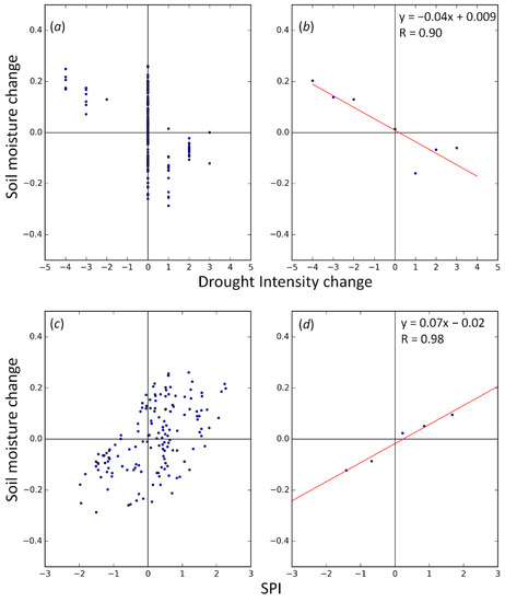
Figure 1.
The scatter plot between 13-week soil moisture changes and 13-week drought intensity changes (a) as observed; and (b) after averaging all of the soil moisture change values corresponding to each drought-intensity change. Similarly, (c,d) show the relationship between 13-week soil moisture change and the three-monthly Standardized Precipitation Index (SPI). These plots were created for a randomly selected grid (27.101°N, 81.224°W) in the contiguous United States (CONUS).
Similarly, the relationship between soil moisture change and SPI were established. Since SPI itself is a measure of deviation from normal rainfall, we used SPI without computing any changes. Hence, the four, 13, and 26-week soil moisture changes were compared against the one, three, and six-monthly SPI values, respectively. Both the soil moisture change and the SPI had continuous values, and since we used three years of data, the scatter between soil moisture change and SPI was quite large, which affected the proper identification of the linear relationship between the two variables. Hence, for each M36 grid, we divided the available SPI data into five equal intervals, and binned the soil moisture change values within each SPI interval. The lower and upper bounds of each SPI class varied based on the data for each grid. The mean of each SPI class and the corresponding soil moisture change values were computed, and these mean values were used to establish the linear regression between soil moisture change and SPI. As an example, the scatter between the 13-week change in soil moisture and the three-month SPI over a randomly selected grid in CONUS is shown in Figure 1c, and the linear relationship between average soil moisture change and average SPI values is shown in Figure 1d. From the figure, it can be observed that the slope of the linear line between soil moisture change and SPI is positive. This implies that the negative value of soil moisture change is associated with a negative SPI value (lower than normal rainfall), and positive soil moisture change is associated with a positive SPI value (higher than normal rainfall).
3. Results
3.1. Comparison of Soil Moisture Change with USDM
The spatial distribution of the slope of the linear regression between the change in soil moisture and the change in USDM drought intensity is presented in Figure 2. Similarly, the spatial distribution of the correlation coefficient of the linear relationship is presented in Figure 3.
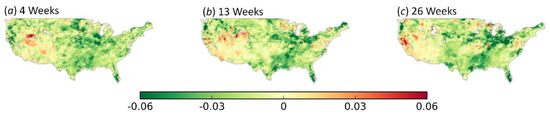
Figure 2.
Slope of the linear regression between the change in soil moisture and the change in drought intensity over CONUS at multiple time intervals: (a) four weeks, (b) 13 weeks, and (c) 26 weeks.
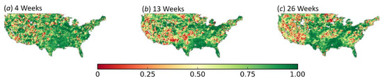
Figure 3.
Correlation coefficient of the linear regression between the change in soil moisture and the change in drought intensity over CONUS at multiple time intervals: (a) four weeks, (b) 13 weeks, and (c) 26 weeks.
From Figure 2, it can be observed that the slope values were more negative in the eastern United States (US) when compared with the Midwest and the western US. The slope values were mostly around zero over the Midwest and the western parts of the country, and further, over small parts of western US, the values were positive. Similarly, the areas with negative slopes exhibited higher correlation (Figure 3), and lower values of correlation were observed over areas with slope values closer to zero or greater than zero. The small white patches in Figure 2 and Figure 3 are the areas where there are not enough data points to statistically determine a slope for the linear regression. Then, we examined randomly selected grids across CONUS to further analyze this pattern of slope values. The analysis revealed that the change in soil moisture was able to indicate the change in drought intensity. An example for this is presented in Figure 4, where the relationship between 26-week soil moisture change and 26-week USDM drought intensity change is presented in the form of scatter plots and a time series over a M36 grid in Arkansas (33.627°N, 94.294°W) (Figure 4a,b) and a grid in Ohio (40.687°N, 80.850°W) (Figure 4c,d). The scatter plots (Figure 4a,c) demonstrate the overall relationship between the two variables, and the time series (Figure 4b,d) clearly indicates the co-variation of the changes in soil moisture and USDM drought intensity. From the time series, it can be observed that a positive soil moisture is immediately reflected in improving drought conditions (negative change in the USDM), and vice versa. It can also be observed that the change in soil moisture and the change in drought intensity almost mirror each other, and the drought intensity change lags behind the soil moisture change by few weeks. This lag time varied for different parts of the CONUS.
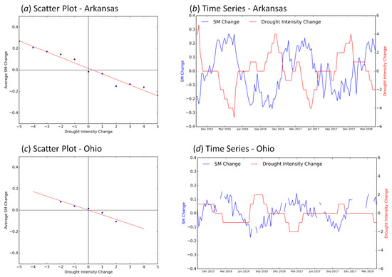
Figure 4.
The relationship between 26-week soil moisture change and 26-week drought intensity change shown in form of (a,c) scatter plots and (b,d) a time series over two selected grids in the CONUS. The gaps in soil moisture in (d) are due to the freezing of the land surface during winter months.
The analysis further indicated that soil moisture change can provide clues about the impending drought conditions. The time series of the changes in soil moisture and the USDM over a grid in Florida (same grid used in Figure 1) is presented in Figure 5. From the 13-week and 26-week changes (Figure 5b,c), it can be observed that the soil moisture is slowly decreasing toward the end of 2016, leading to drought-like conditions that lasted up to June 2017. However, this trend was not observed in the four-week change plot (Figure 5a). This also indicates that the change analysis needs to be done at multiple time scales in order not to miss the signals of drought.
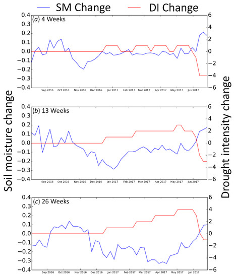
Figure 5.
Time series of soil moisture and drought intensity changes over a grid in Florida (27.101°N, 81.224°W) at (a) four-week, (b) 13-week, and (c) 26-week time intervals. In the figure, DI indicates drought intensity.
Another example of the soil moisture change indicating the change in drought conditions is presented in Figure 6. In the figure, the USDM maps published on 17 April 2018 (Figure 6a) and 10 October 2017 (Figure 6b) are shown. The time periods are selected such that they are 26 weeks apart. In Figure 6c, the soil moisture change observed over the Southern states (indicated with a red rectangle in Figure 6a,b) over the same time interval is shown. From the figures, it is strikingly clear that the areas where the drought conditions had intensified in April 2018 in comparison with October 2017 (over parts of Kansas, West Oklahoma, and West Texas) are associated with a negative soil moisture change (indicated with yellow and red shades in Figure 6c), and the areas where the drought conditions had improved (over parts of Missouri, Arkansas, and Louisiana, East Texas, and East Oklahoma) are associated with a positive soil moisture change (indicated with blue shades in Figure 6c). The areas with closer to zero change (indicated with green shade in Figure 6c) in the drought-affected regions were actually dry during 10 October 2017. Since those grids were dry in the starting time itself, they did not show any major changes in the soil moisture value during April 2018.
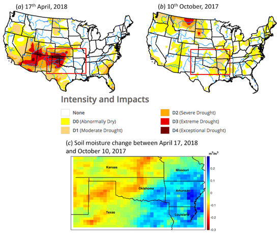
Figure 6.
An example showing how the change in soil moisture responds to the change in drought conditions over the southern United States (USA). The United States Drought Monitor (USDM) maps are downloaded from the drought monitor website http://droughtmonitor.unl.edu.
3.2. Comparison of Soil Moisture Change with SPI
The soil moisture change is then compared with the SPI to assess whether the temporal pattern of SPI is reflected in the change in soil moisture. As explained in Section 2.4, the linear regression between soil moisture change and SPI is expected to have a positive slope. Figure 7 and Figure 8 present the spatial pattern of the slope and correlation of the linear regression between soil moisture change and SPI across CONUS for multiple time intervals, respectively. Similar to the relationship between soil moisture change and the USDM, the slope of linear regression between soil moisture change and SPI were more positive in the eastern and central US than in the western US. Further, it can be observed from Figure 8 that the SPI and soil moisture change exhibit a higher correlation between them over most parts of the CONUS at the four-week interval than the 13- or 26-week intervals. This indicates a stronger relationship between the SMAP soil moisture change and rainfall at monthly time intervals.
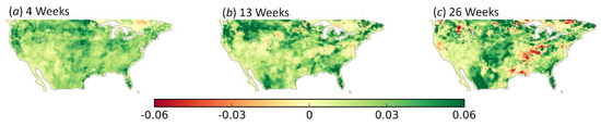
Figure 7.
Slope of the linear regression between the change in soil moisture and the Standardized Precipitation Index (SPI) over CONUS at multiple time intervals (a) four weeks, (b) 13 weeks, and (c) 26 weeks.
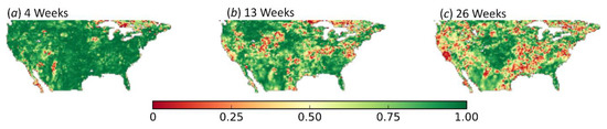
Figure 8.
Spatial distribution of the correlation between the change in soil moisture and SPI over CONUS at multiple time intervals (a) four weeks, (b) 13 weeks, and (c) 26 weeks.
To further understand the relationship between soil moisture change and SPI, a time series of these two variables at multiple time intervals were plotted over Florida (same spatial grid used in Figure 5), which is presented in Figure 9. It can be observed from Figure 9a that the four-week soil moisture change and one-month SPI follow each other very closely, and at 13-week (Figure 9b) and 26-week (Figure 9c) intervals, they both exhibit very similar overall trends, though they do not match each other closely. However, from Figure 9c, it can also be observed that both the 26-week soil moisture change interval and the six-monthly SPI exhibit a negative trend from November 2016 to June 2017, indicating worsening drought conditions. This confirms the earlier observation that the soil moisture change analysis at multiple time intervals complement each other in providing signals about drought conditions.
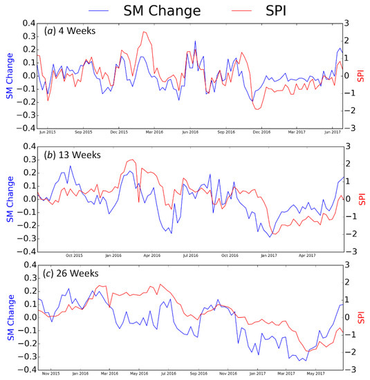
Figure 9.
Time series of soil moisture change and SPI over a grid in Florida (27.101°N, 81.224°W). The plots (a–c) indicate the comparison of four-week, 13-week, and 26-week soil moisture change intervals with one, three, and six-monthly SPI intervals, respectively.
After analyzing the relationship between soil moisture change, the USDM, and the SPI, we analyzed the data to find out the reasons for the occurrence of the near-zero slope and lower correlation values over the western US. The information carried by this linear regression-based analysis was limited when the average soil moisture change values corresponding to different drought intensity changed values, or the SPI became closer to zero. This is illustrated in Figure 10, in which the soil moisture change and drought intensity change values over a grid in Arizona are plotted. From the time series (Figure 10b), it can be observed that the soil moisture change was smaller in magnitude and exhibited rapid changes without following any temporal cycles. This suggested that the grid was dry throughout the time period of data analysis leading to a closer-to-zero slope (Figure 10a). Hence, for regions that are either dry or wet throughout, the analysis of soil moisture change may not provide any additional information. However, when there is a sudden decrease in soil moisture over a wet region, or when the soil moisture suddenly increases over a dry region, the change analysis can pick up these anomalies, indicating a change in the overall conditions. Further, it was observed that over regions with high-intensity agriculture with irrigation water supply, the soil moisture change exhibited corresponding trends with the cropping cycle. As an illustration, the data over a M36 grid in the central valley in California is presented in Figure 11. In the time series plots between soil moisture change and drought intensity change (Figure 11b) and soil moisture change and the SPI (Figure 11d), it can be observed that the drought conditions were worsening, as indicated by the positive drought intensity change, and the rainfall was much lower than normal, as indicated by the negative SPI during the period between November 2017 and March 2018 (marked by a black oval shape). However, the 26-week soil moisture change was positive, indicating that additional water was supplied to the crops to sustain their growth. This positive soil moisture change during the dry period influenced the regression between soil moisture change and drought intensity change (Figure 11a), and soil moisture change and the SPI (Figure 11c), changing the direction of the slope.
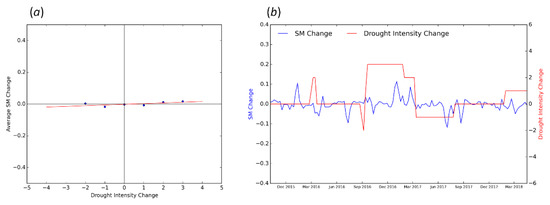
Figure 10.
The relationship between 26-week soil moisture change and 26-week drought intensity change, shown in form of (a) a scatter plot and (b) a time series over Arizona (32.288°N, 114.087°W).
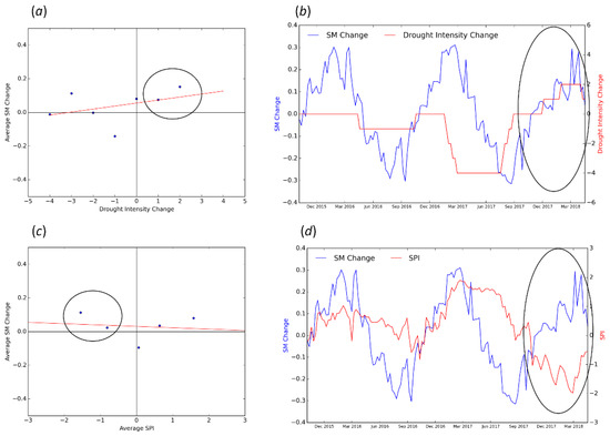
Figure 11.
The relationship between 26-week soil moisture change and 26-week drought intensity change (plots (a,b)), and the relationship between 26-week soil moisture change and six-month SPI (plots (c,d)) over the central valley in California (37.077°N, 120.436°W).
4. Discussions
The data analysis revealed that soil moisture change was able to track the change in drought conditions over most parts of the CONUS. It was further observed that the soil moisture change at relatively longer intervals (13 weeks or 26 weeks) was able to identify the change in drought conditions, as indicated by the USDM drought intensity index. On the other hand, short-term soil moisture change (over four weeks) more closely resembled the one-month SPI. Scaini et al. [10] also observed good correlation between soil moisture anomalies from the SMOS satellite and the SPI estimated at 30 to 50-day intervals. In addition, previous studies demonstrated that short-term SPI (one to three months) had higher correlation with soil moisture measurements made at 10-cm depth [35], and long-term SPI are correlated with soil moisture at deeper layers of the strata [33]. These results suggest that soil moisture change estimated at multiple time intervals complement each other and provide information about varying drought conditions. For example, a short-term decrease (over four weeks) in soil moisture may indicate a decrease in precipitation over the time period, whereas a persistently negative soil moisture change over a relatively longer time interval (13 weeks or 26 weeks) could indicate agricultural drought. It is to be noted that the maximum time period considered for change analysis was limited to six months in this study for the sake of simplicity and clarity. However, during very long periods of persistent droughts (lasting for one year or more), change analysis done for periods less than a year may not provide much valuable information. Hence, the time period considered for change analysis can be varied between one month and 24 months, or even more for practical applications similar to the use of long-term SPI (24 months and 60 months) in the development of the USDM long-term drought impact maps [31].
Previous studies noted a lag between USDM drought intensity and actual ground conditions. Further, it was also noted that if long-term drought indicators are really dry (wet), the USDM will indicate drought (non-drought) conditions, even if recent rainfall (lack of recent rainfall) had improved (worsened) the water availability and cropping conditions [32]. This nature of USDM might have also affected the slope of linear regression between soil moisture change and the change in drought intensity over western US, which is recovering from a long-term drought. The soil moisture observed by the SMAP corresponds to the moisture content at the top few centimeters of the soil [21]. However, a recent study [9] demonstrated that this top surface soil moisture from SMAP show a strong relationship with soil moisture measurements made up to 20-cm depth. Further, the soil moisture ‘persistence’ or ‘memory’ on the surface can influence the land–atmosphere interaction and associated feedbacks [1,36]. These results suggest that the surface soil moisture information is vital for understanding the duration and intensity of droughts. In addition, the onset and withdrawal of droughts is normally preceded by decreasing and increasing soil moisture values for a considerable period of time. Hence, the regular monitoring of soil moisture change can potentially indicate the onset and recovery of drought events.
5. Conclusions
This study aimed to understand how the soil moisture change observed from the SMAP satellite responds to drought conditions over multiple time intervals. This was done by comparing the change in soil moisture with the change in USDM drought intensity values, and further with the SPI at multiple time intervals. The results indicated that soil moisture change may provide valuable information about the change in drought conditions. This study is a preliminary exercise to demonstrate the potential of SMAP soil moisture change for drought analysis, and this study further demonstrated that soil moisture change can provide valuable information about the change in drought intensity, as indicated by the USDM. Hence, a proper framework should be developed for ingesting this soil moisture change information into the various existing drought-monitoring tools, such as the USDM, and multivariate drought indices. Further studies should be carried out across the globe to see how soil moisture change signals about droughts of varying severity and duration. In addition, a subsequent study will focus on the combined use of vapor pressure deficit, precipitation anomalies, and soil moisture change for improving drought monitoring and analysis.
Author Contributions
E.R. and N.N.D. conceived the work; E.R. did the analysis with inputs from N.N.D., M.S., D.E. and A.B.; The SPI data was provided by C.P. and J.S.; The initial draft of the manuscript was written by E.R.; All the others contributed to the final version.
Acknowledgments
This work is supported by NASA HQ Earth Science Application: Water Resources Program, and Water and Energy Cycle: Terrestrial Hydrology Program. The Authors thank the three reviewers and the Editor for their comments that helped improving the manuscript.
Conflicts of Interest
The Authors declare no conflict of interest.
Appendix A
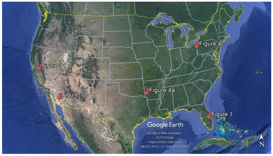
Figure A1.
Location of different grid points used as examples in various figures in the main text. The Label of each grid point refers to the corresponding figure in the main text. (Image courtesy: Google Earth™).
References
- Seneviratne, S.I.; Corti, T.; Davin, E.L.; Hirschi, M.; Jaeger, E.B.; Lehner, I.; Orlowsky, B.; Teuling, A.J. Investigating soil moisture—Climate interactions in a changing climate: A review. Earth-Sci. Rev. 2010, 99, 125–161. [Google Scholar] [CrossRef]
- Karthikeyan, L.; Pan, M.; Wanders, N.; Kumar, D.N.; Wood, E.F. Four decades of microwave satellite soil moisture observations: Part 2. Product validation and inter-satellite comparisons. Adv. Water Resour. 2017, 109, 236–252. [Google Scholar] [CrossRef]
- Mishra, A.; Vu, T.; Veettil, A.V.; Entekhabi, D. Drought monitoring with soil moisture active passive (SMAP) measurements. J. Hydrol. 2017, 552, 620–632. [Google Scholar] [CrossRef]
- Nicolai-Shaw, N.; Zscheischler, J.; Hirschi, M.; Gudmundsson, L.; Seneviratne, S.I. A drought event composite analysis using satellite remote-sensing based soil moisture. Remote Sens. Environ. 2017, 203, 216–225. [Google Scholar] [CrossRef]
- Zargar, A.; Sadiq, R.; Naser, B.; Khan, F.I. A review of drought indices. Environ. Rev. 2011, 19, 333–349. [Google Scholar] [CrossRef]
- Hao, Z.; Singh, V.P. Drought characterization from a multivariate perspective: A review. J. Hydrol. 2015, 527, 668–678. [Google Scholar] [CrossRef]
- Hao, Z.; Yuan, X.; Xia, Y.; Hao, F.; Singh, V.P. An Overview of Drought Monitoring and Prediction Systems at Regional and Global Scales. Bull. Am. Meteorol. Soc. 2017, 98, 1879–1896. [Google Scholar] [CrossRef]
- Seneviratne, S.; Nicholls, N.; Easterling, D.; Goodess, C.; Kanae, S.; Kossin, J.; Zwiers, F. Changes in Climate Extremes and their Impacts on the Natural Physical Environment. In Managing the Risks of Extreme Events and Disasters to Advance Climate Change Adaptation: Special Report of the Intergovernmental Panel on Climate Change; Field, C., Barros, V., Stocker, T., Dahe, Q., Eds.; Cambridge University Press: Cambridge, UK, 2012; pp. 109–230. [Google Scholar] [CrossRef]
- Velpuri, N.M.; Senay, G.B.; Morisetter, J.T. Evaluating new SMAP soil moisture for drought monitoring in the rangelands of the US high plains. Rangelands 2016, 38, 183–190. [Google Scholar] [CrossRef]
- Scaini, A.; Sanchez, N.; Vicente-Serrano, S.M.; Martínez-Fernández, J. SMOS-derived soil moisture anomalies and drought indices: A comparative analysis using in situ measurements. Hydrol. Process. 2015, 29, 373–383. [Google Scholar] [CrossRef]
- Hunt, E.D.; Hubbard, K.G.; Wilhite, D.A.; Arkebauer, T.J.; Dutcher, A.L. The development and evaluation of a soil moisture index. Int. J. Climatol. 2009, 29, 747–759. [Google Scholar] [CrossRef]
- Martínez-Fernández, J.; González-Zamora, A.; Sánchez, N.; Gumuzzio, A. A soil water based index as a suitable agricultural drought indicator. J. Hydrol. 2015, 522, 265–273. [Google Scholar] [CrossRef]
- Martínez-Fernández, J.; González-Zamora, A.; Sanchez, N.; Gumuzzio, A.; Herrero-Jiménez, C.M. Satellite soil moisture for agricultural drought monitoring: Assessment of the SMOS derived Soil Water Deficit Index. Remote Sens. Environ. 2016, 177, 277–286. [Google Scholar] [CrossRef]
- Carrao, H.; Russo, S.; Sepulcre-Canto, G.; Barbosa, P. An empirical standardized soil moisture index for agricultural drought assessment from remotely sensed data. Int. J. Appl. Earth Obs. Geoinf. 2016, 48, 74–84. [Google Scholar] [CrossRef]
- Sánchez, N.; González-Zamora, Á.; Piles, M.; Martínez-Fernández, J. A New Soil Moisture Agricultural Drought Index (SMADI) Integrating MODIS and SMOS Products: A Case of Study over the Iberian Peninsula. Remote Sens. 2016, 8, 287. [Google Scholar] [CrossRef]
- Cammalleri, C.; Micale, F.; Vogt, J. A novel soil moisture-based drought severity index (DSI) combining water deficit magnitude and frequency. Hydrol. Process. 2016, 30, 289–301. [Google Scholar] [CrossRef]
- Dorigo, W.; de Jeu, R. Satellite soil moisture for advancing our understanding of earth system processes and climate change. Int. J. Appl. Earth Obs. Geoinf. 2016, 48, 1–4. [Google Scholar] [CrossRef]
- Dorigo, W.; Wagner, W.; Albergel, C.; Albrecht, F.; Balsamo, G.; Brocca, L.; Chung, D.; Ertl, M.; Forkel, M.; Gruber, A.; et al. ESA CCI Soil Moisture for improved Earth system understanding: State-of-the art and future directions. Remote Sens. Environ. 2017, 203, 185–215. [Google Scholar] [CrossRef]
- Choi, M.; Jacobs, J.M.; Anderson, M.C.; Bosh, D.D. Evaluation of drought indices via remotely sensed data with hydrological variables. J. Hydrol. 2013, 476, 265–273. [Google Scholar] [CrossRef]
- Sheffield, J.; Goteti, G.; Wen, F.; Wood, E.F. A simulated soil moisture based drought analysis for the United States. J. Geophys. Res. 2004, 109, D24108. [Google Scholar] [CrossRef]
- Rondinelli, W.J.; Hornbuckle, B.K.; Patton, J.C.; Cosh, M.H.; Walker, V.A.; Carr, B.D.; Logsdon, S.D. Different Rates of Soil Drying after Rainfall Are Observed by the SMOS Satellite and the South Fork in situ Soil Moisture Network. J. Hydrometeorol. 2015, 16, 889–903. [Google Scholar] [CrossRef]
- Eltahir, E.A.B.; Yeh, P.J.F. On the asymmetric response of aquifer water level to floods and droughts in Illinois. Water Resour. Res. 1999, 35, 1199–1217. [Google Scholar] [CrossRef]
- Shellito, P.J.; Small, E.E.; Colliander, A.; Bindlish, R.; Cosh, M.H.; Berg, A.A.; Bosch, D.D.; Caldwell, T.G.; Goodrich, D.C.; McNairn, H.; et al. SMAP soil moisture drying more rapid than observed in situ following rainfall events. Geophys. Res. Lett. 2016, 43, 8068–8075. [Google Scholar] [CrossRef]
- Svoboda, M.D.; LeComte, D.; Hayes, M.; Heim, R.; Gleason, K.; Angel, J.; Rippey, B.; Tinker, R.; Palecki, M.; Stooksbury, D.; et al. The Drought Monitor. Bull. Am. Meteorol. Soc. 2002, 83, 1181–1190. [Google Scholar] [CrossRef]
- McKee, T.B.; Doesken, N.J.; Kleist, J. The relationship of drought frequency and duration to time scales. In Proceedings of the Eighth Conference on Applied Climatology, Anaheim, CA, USA, 17–22 January 1993. [Google Scholar]
- Entekhabi, D.; Yueh, S.; O’Neill, P.E.; Kellogg, K.H.; Allen, A.; Bindlish, R.; Brown, M.; Chan, S.; Colliander, A.; Crow, W.T.; et al. SMAP Handbook—Soil Moisture Active Passive: Mapping Soil Moisture and Freeze/Thaw from Space; Jet Propulsion Laboratory, California Institute of Technology: Pasadena, CA, USA, 2014. [Google Scholar]
- Brown, M.E.; Escobar, V.; Moran, S.; Entekhabi, D.; O’Neil, P.E.; Njoku, E.G.; Doorn, B.; Entin, J.K. NASA’s soil moisture Active Passive (SMAP) Mission and opportunities for application users. Bull. Am. Meteorol. Soc. 2013, 1125–1128. [Google Scholar] [CrossRef]
- Colliander, A.; Jackson, T.J.; Bindlish, R.; Chan, S.; Das, N.; Kim, S.B.; Cosh, M.H.; Dunbar, R.S.; Dang, L.; Pashaian, L.; et al. Validation of SMAP surface soil moisture products with core validation sites. Remote Sens. Environ. 2017, 191, 215–231. [Google Scholar] [CrossRef]
- Brodzik, M.J.; Billingsley, B.; Haran, T.; Raup, B.; Savoie, M.H. EASE-Grid 2.0: Incremental but Significant Improvements for Earth-Gridded Data Sets. ISPRS Int. J. Geo-Inf. 2012, 1, 32–45. [Google Scholar] [CrossRef]
- O’Neill, P.; Chan, S.; Njoku, E.; Jackson, T.; Bindlish, R. Algorithm Theoretical Basis Document Level 2 & 3 Soil Moisture (Passive) Data Products; Jet Propulsion Laboratory, California Institute of Technology: Pasadena, CA, USA, 2015. [Google Scholar]
- Anderson, M.C.; Hain, C.; Otkin, J.; Zhan, X.; Mo, K.; Svoboda, M.; Wardlow, B.; Pimstein, A. An intercomparison of drought indicators based on thermal remote sensing and NLDAS-2 simulations with U.S Drought Monitor classifications. J. Hydrometeorol. 2013, 14, 1035–1056. [Google Scholar] [CrossRef]
- Lorenz, D.J.; Otkin, J.A.; Svoboda, M.; Hain, C.R.; Anderson, M.C.; Zhong, Y. Predicting US drought monitor states using precipitation, soil moisture and evapotranspiration anomalies. Part-I Development of a non-discrete USDM Index. J. Hydrometeorol. 2017, 18, 1943–1962. [Google Scholar] [CrossRef]
- Spennemann, P.C.; Rivera, J.A.; Saulo, A.C.; Penalba, O.C. A Comparison of GLDAS Soil Moisture Anomalies against Standardized Precipitation Index and Multisatellite Estimations over South America. J. Hydrometeorol. 2015, 16, 158–171. [Google Scholar] [CrossRef]
- World Meteorological Organization (WMO). Standardized Precipitation Index User Guide, WMO 1090, 24. 2012. Available online: www.wamis.org/agm/pubs/SPI/WMO_1090_EN.pdf (accessed on 20 February 2018).
- Sims, A.P.; Niyogi, D.S.; Raman, S. Adopting drought indices for estimating soil moisture: A North Carolina case study. Geophys. Res. Lett. 2002, 29, 1183. [Google Scholar] [CrossRef]
- Mccoll, K.A.; Alemohammad, S.H.; Akbar, R.; Yueh, S.; Entekhabi, D. The global distribution and dynamics of surface soil moisture. Nat. Geosci. 2017, 10, 100–104. [Google Scholar] [CrossRef]
© 2018 by the authors. Licensee MDPI, Basel, Switzerland. This article is an open access article distributed under the terms and conditions of the Creative Commons Attribution (CC BY) license (http://creativecommons.org/licenses/by/4.0/).