Comparing Landsat and RADARSAT for Current and Historical Dynamic Flood Mapping

Abstract

1. Introduction
2. Materials and Methods
2.1. Data
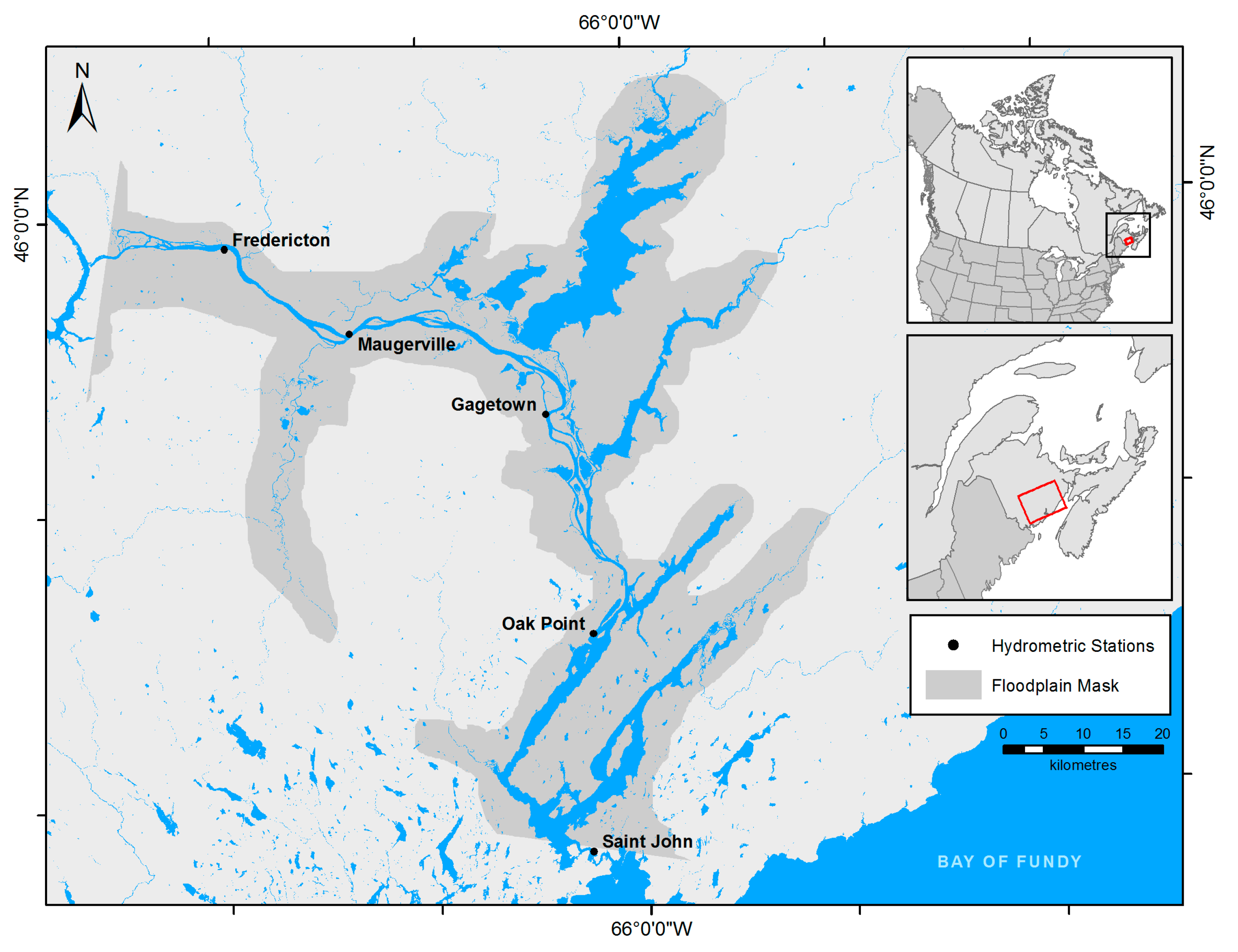
2.1.1. Study Area
2.1.2. Landsat
2.1.3. RADARSAT
2.1.4. Hydrometric Data
2.1.5. High-Resolution Imagery
2.2. Flood Mapping
2.2.1. Landsat
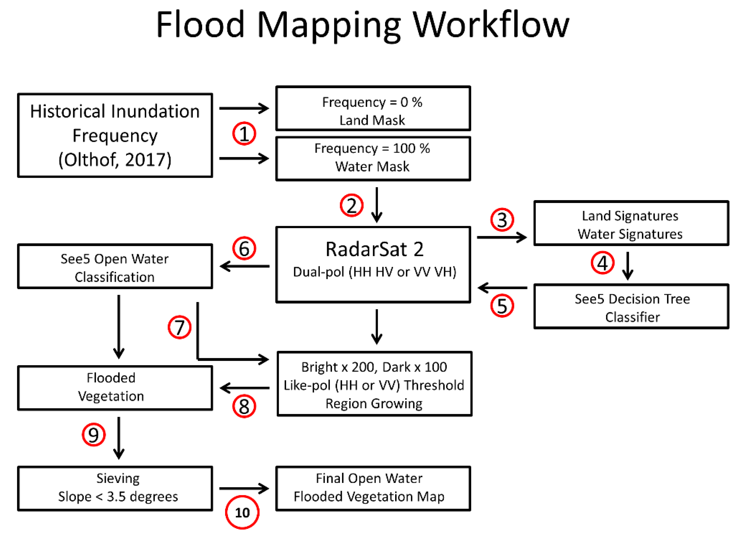
2.2.2. RADARSAT
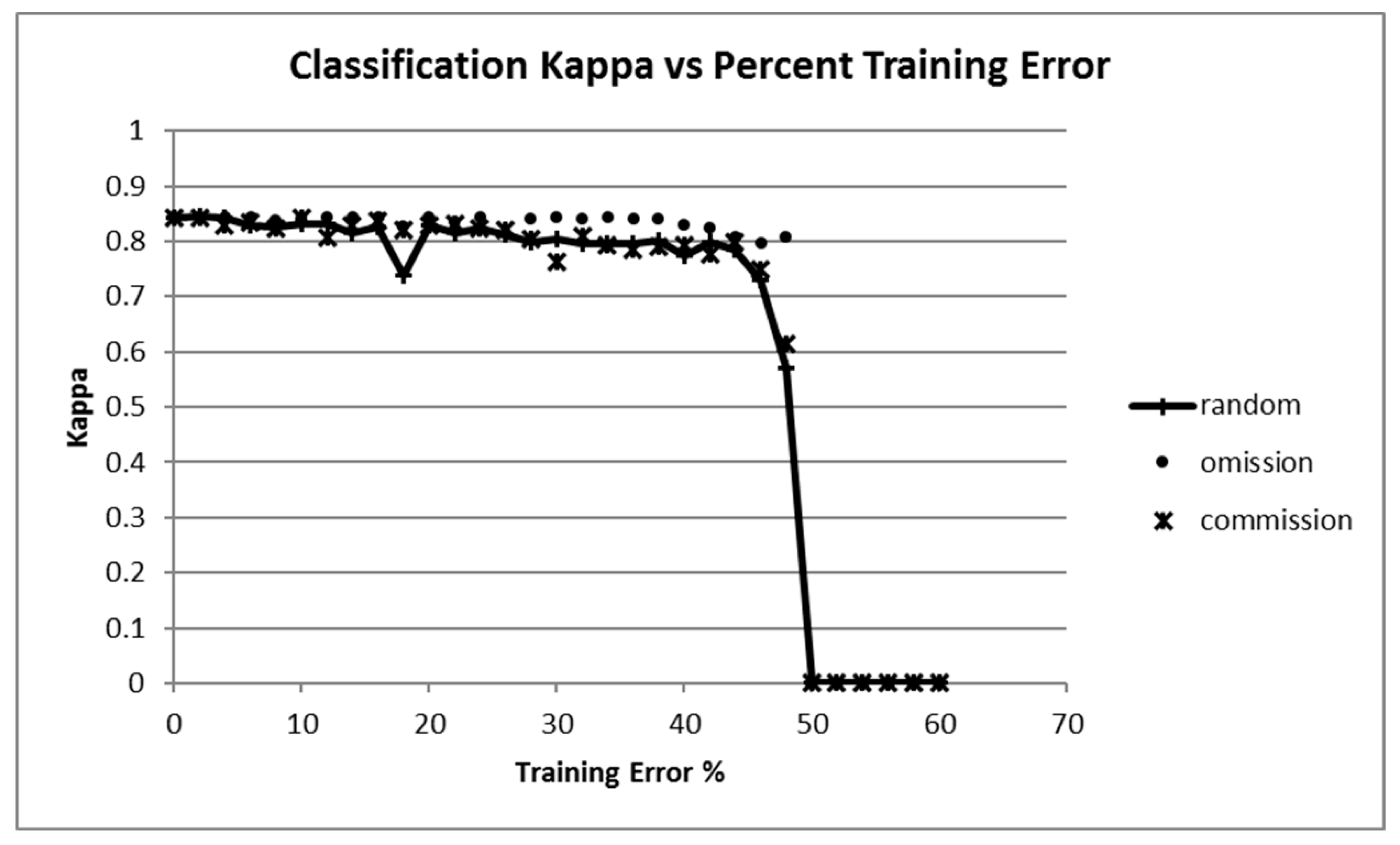
2.3. Sensitivity of RADARSAT 2 Open Water Mapping to Training Error
2.4. Surface Water Dynamics
2.4.1. Inundation Frequency
2.4.2. Inundation Trends
3. Results
3.1. Training Error
3.2. Comparison between RADARSAT 2 and Landsat Flood Extents
3.3. Comparisons between Mapped Flood Extents and Hydrometric Water Depth
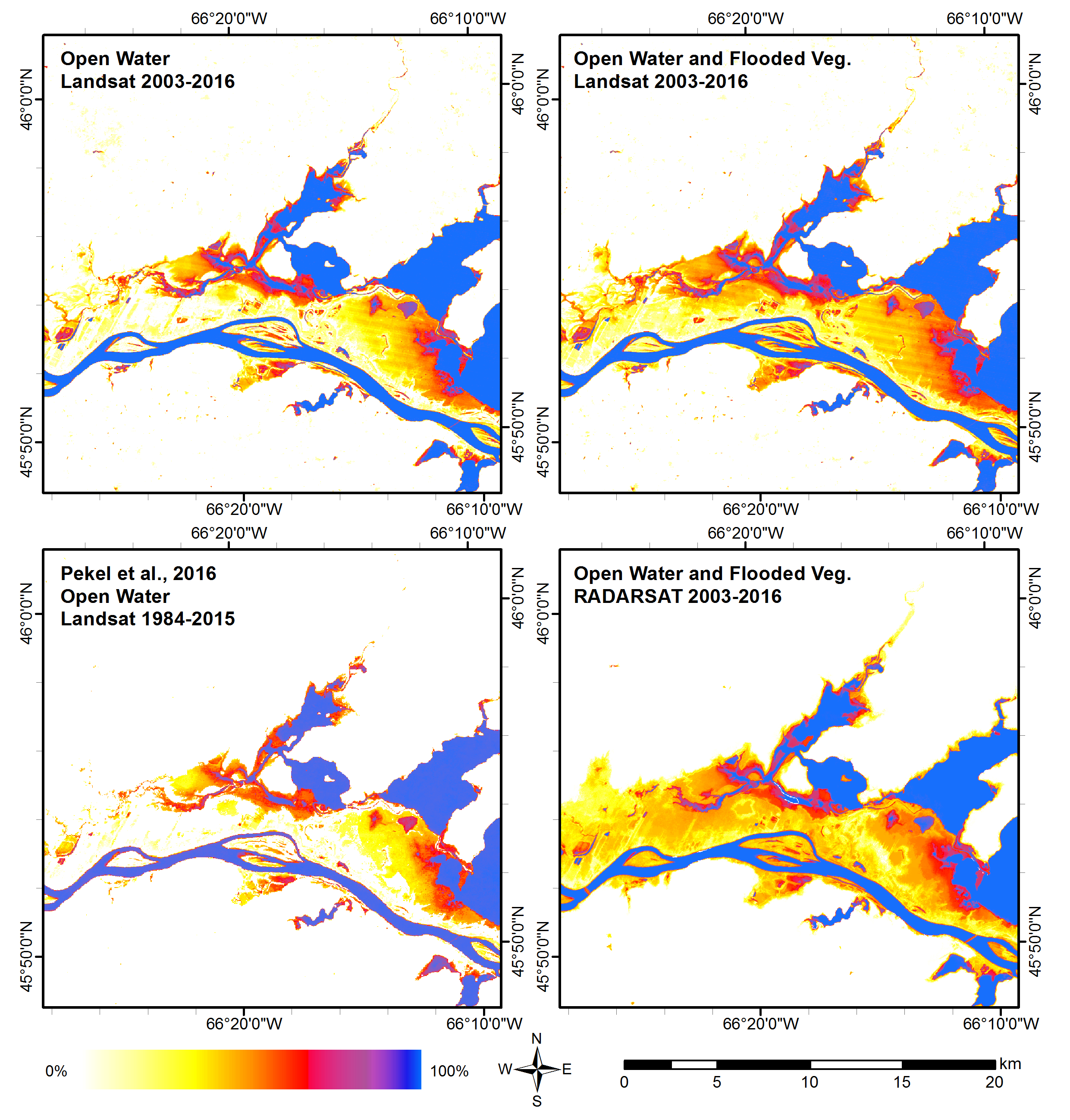
3.4. Inundation Frequencies
3.5. Inundation Trends
4. Discussion
5. Conclusions
Author Contributions
Acknowledgments
Conflicts of Interest
References
- Intergovernmental Panel on Climate Change. Climate Change 2013—The Physical Science Basis: Working Group I Contribution to the Fifth Assessment Report of the Intergovernmental Panel on Climate Change; Intergovernmental Panel on Climate Change, Ed.; Cambridge University Press: Cambridge, UK, 2014; ISBN 978-1-107-41532-4. [Google Scholar]
- Thomas, R.F.; Kingsford, R.T.; Lu, Y.; Hunter, S.J. Landsat mapping of annual inundation (1979–2006) of the Macquarie Marshes in semi-arid Australia. Int. J. Remote Sens. 2011, 32, 4545–4569. [Google Scholar] [CrossRef]
- Olthof, I. Mapping Seasonal Inundation Frequency (1985–2016) along the St-John River, New Brunswick, Canada using the Landsat Archive. Remote Sens. 2017, 9, 143. [Google Scholar] [CrossRef]
- Mueller, N.; Lewis, A.; Roberts, D.; Ring, S.; Melrose, R.; Sixsmith, J.; Lymburner, L.; McIntyre, A.; Tan, P.; Curnow, S.; et al. Water observations from space: Mapping surface water from 25 years of Landsat imagery across Australia. Remote Sens. Environ. 2016, 174, 341–352. [Google Scholar] [CrossRef]
- Verpoorter, C.; Kutser, T.; Seekell, D.A.; Tranvik, L.J. A global inventory of lakes based on high-resolution satellite imagery. Geophys. Res. Lett. 2014, 41, 2014GL060641. [Google Scholar] [CrossRef]
- Feng, M.; Sexton, J.O.; Channan, S.; Townshend, J.R. A global, high-resolution (30-m) inland water body dataset for 2000: First results of a topographic–spectral classification algorithm. Int. J. Digit. Earth 2016, 9, 113–133. [Google Scholar] [CrossRef]
- Yamazaki, D.; Trigg, M.A.; Ikeshima, D. Development of a global ~90 m water body map using multi-temporal Landsat images. Remote Sens. Environ. 2015, 171, 337–351. [Google Scholar] [CrossRef]
- Prigent, C.; Papa, F.; Aires, F.; Jimenez, C.; Rossow, W.B.; Matthews, E. Changes in land surface water dynamics since the 1990s and relation to population pressure. Geophys. Res. Lett. 2012, 39, L08403. [Google Scholar] [CrossRef]
- Brisco, B.; Short, N.; van der Sanden, J.; Landry, R.; Raymond, D. A semi-automated tool for surface water mapping with Radarsat-1. Can. J. Remote Sens. 2009, 35, 336–344. [Google Scholar]
- Wang, Y.; Colby, J.D.; Mulcahy, K.A. An efficient method for mapping flood extent in a coastal floodplain using Landsat TM and DEM data. Int. J. Remote Sens. 2002, 23, 3681–3696. [Google Scholar] [CrossRef]
- Martinis, S.; Rieke, C. Backscatter Analysis Using Multi-Temporal and Multi-Frequency SAR Data in the Context of Flood Mapping at River Saale, Germany. Remote Sens. 2015, 7, 7732–7752. [Google Scholar] [CrossRef]
- Yu, Y.; Saatchi, S. Sensitivity of L-Band SAR Backscatter to Aboveground Biomass of Global Forests. Remote Sens. 2016, 8, 522. [Google Scholar] [CrossRef]
- Mackey, H.E., Jr.; Riley, R.S. Mapping of flood patterns in a 10,000-acre southeastern river swamp with SPOT HRV data. In ASPRS/ACSM Annual Convention and Exposition; Technical Paper 1; ASPRS: Reno, Nevada, 1994; p. 375. [Google Scholar]
- Townsend, P.A.; Walsh, S.J. Modeling floodplain inundation using an integrated GIS with radar and optical remote sensing. Gemorphology 1998, 21, 295–312. [Google Scholar] [CrossRef]
- Lang, M.; McCarty, G.; Oesterling, R.; Yeo, I.-Y. Topographic Metrics for Improved Mapping of Forested Wetlands. Wetlands 2013, 33, 141–155. [Google Scholar] [CrossRef]
- Roy, D.P.; Zhang, H.K.; Ju, J.; Gomez-Dans, J.L.; Lewis, P.E.; Schaaf, C.B.; Sun, Q.; Li, J.; Huang, H.; Kovalskyy, V. A general method to normalize Landsat reflectance data to nadir BRDF adjusted reflectance. Remote Sens. Environ. 2016, 176, 255–271. [Google Scholar] [CrossRef]
- White, L.; Brisco, B.; Dabboor, M.; Schmitt, A.; Pratt, A. A Collection of SAR Methodologies for Monitoring Wetlands. Remote Sens. 2015, 7, 7615–7645. [Google Scholar] [CrossRef]
- Freeman, A.; Durden, S.L. A three-component scattering model for polarimetric SAR data. IEEE Trans. Geosci. Remote Sens. 1998, 36, 963–973. [Google Scholar] [CrossRef]
- Hess, L.L.; Melack, J.M.; Simonett, D.S. Radar detection of flooding beneath the forest canopy: A review. Int. J. Remote Sens. 1990, 11, 1313–1325. [Google Scholar] [CrossRef]
- Lang, M.; Townsend, P.; Kasischke, E. Influence of incidence angle on detecting flooded forests using C-HH synthetic aperture radar data. Remote Sens. Environ. 2008, 112, 3898–3907. [Google Scholar]
- Bolanos, S.; Stiff, D.; Brisco, B.; Pietroniro, A. Operational surface water detection and monitoring using RADARSAT 2. Remote Sens. 2016, 8, 285. [Google Scholar] [CrossRef]
- O’Grady, D.; Leblanc, M.; Gillieson, D. Relationship of local incidence angle with satellite radar backscatter for different surface conditions. Int. J. Appl. Earth Obs. Geoinf. 2013, 24, 42–53. [Google Scholar]
- Li, J.; Wang, S. An automatic method for mapping inland surface waterbodies with RADARSAT-2 imagery. Int. J. Remote Sens. 2015, 36, 1367–1384. [Google Scholar] [CrossRef]
- Woodhouse, I.H. Introduction to Microwave Remote Sensing; CRC Press: Boca Raton, FL, USA, 2005. [Google Scholar]
- Henry, J.-B.; Chastanet, P.; Fellah, K.; Desnos, Y.-L. Envisat multi-polarized ASAR data for flood mapping. Int. J. Remote Sens. 2006, 27, 1921–1929. [Google Scholar] [CrossRef]
- White, L.; Brisco, B.; Pregitzer, M.; Tedford, B.; Boychuk, L. RADARSAT-2 Beam Mode Selection for Surface Water and Flooded Vegetation Mapping. Can. J. Remote Sens. 2014, 40, 135–151. [Google Scholar] [CrossRef]
- Schowengerdt, R.A. Remote Sensing, Third Edition: Models and Methods for Image Processing, 3rd ed.; Academic Press: Burlington, MA, USA, 2006; ISBN 978-0-12-369407-2. [Google Scholar]
- Pax-Lenney, M.; Woodcock, C.E.; Macomber, S.A.; Gopal, S.; Song, C. Forest mapping with a generalized classifier and Landsat TM data. Remote Sens. Envion. 2001, 77, 241–250. [Google Scholar] [CrossRef]
- Song, C.; Woodcock, C.E. Monitoring forest succession with multitemporal Landsat images: Factors of uncertainty. IEEE Trans. Geosci. Remote Sens. 2003, 41, 2557–2567. [Google Scholar] [CrossRef]
- Pekel, J.-F.; Cottam, A.; Gorelick, N.; Belward, A.S. High-resolution mapping of global surface water and its long-term changes. Nature 2016, 540, 418–422. [Google Scholar] [CrossRef] [PubMed]
- Kuenzer, C.; Guo, H.; Huth, J.; Leinenkugel, P.; Li, X.; Dech, S. Flood Mapping and Flood Dynamics of the Mekong Delta: ENVISAT-ASAR-WSM Based Time Series Analyses. Remote Sens. 2013, 5, 687–715. [Google Scholar] [CrossRef]
- Zhu, Z.; Wang, S.; Woodcock, C.E. Improvement and expansion of the Fmask algorithm: Cloud, cloud shadow, and snow detection for Landsats 4–7, 8, and Sentinel 2 images. Remote Sens. Environ. 2015, 159, 269–277. [Google Scholar] [CrossRef]
- Chander, G.; Markham, B.L.; Helder, D.L. Summary of current radiometric calibration coefficients for Landsat MSS, TM, ETM+, and EO-1 ALI sensors. Remote Sens. Environ. 2009, 113, 893–903. [Google Scholar] [CrossRef]
- Quinlan, J.R. C4.5: Programs for Machine Learning; Morgan Kaufmann Publishers Inc.: San Francisco, CA, USA, 1993; ISBN 978-1-55860-238-0. [Google Scholar]
- Ali, I.; Greifeneder, F.; Stamenkovic, J.; Neumann, M.; Notarnicola, C. Review of Machine Learning Approaches for Biomass and Soil Moisture Retrievals from Remote Sensing Data. Remote Sens. 2015, 7, 16398–16421. [Google Scholar] [CrossRef]
- Latifovic, R.; Pouliot, D.; Olthof, I. Circa 2010 land cover of Canada: Local optimization methodology and product development. Remote Sens. 2017, 9, 1098. [Google Scholar] [CrossRef]
- Kasischke, E.S.; Melack, J.M.; Dobson, C. The use of imaging radars for ecological applications—A review. Remote Sens. Environ. 1997, 39, 141–156. [Google Scholar] [CrossRef]
- Ghosh, A.; Manwani, N.; Sastry, P.S. On the Robustness of Decision Tree Learning under Label Noise. arXiv, 2016; arXiv:1605.06296. [Google Scholar]
- Cohen, J. A coefficient of agreement for nominal scales. Educ. Psychol. Meas. 1960, 20, 37–46. [Google Scholar] [CrossRef]
- Myneni, R.B.; Keeling, C.D.; Tucker, C.J.; Asrar, G.; Nemani, R.R. Increased plant growth in the northern high latitudes from 1981 to 1991. Nature 1997, 386, 698–702. [Google Scholar] [CrossRef]
- Pouliot, D.; Latifovic, R.; Olthof, I. Trends in vegetation NDVI from 1 km AVHRR data over Canada for the period 1985–2006. Int. J. Remote Sens. 2009, 30, 149–168. [Google Scholar] [CrossRef]
- Olthof, I.; Fraser, R.H.; Schmitt, C. Landsat-based mapping of thermokarst lake dynamics on the Tuktoyaktuk Coastal Plain, Northwest Territories, Canada since 1985. Remote Sens. Environ. 2015, 168, 194–204. [Google Scholar] [CrossRef]
- Buermann, W.; Wang, Y.; Dong, J.; Zhou, L.; Zeng, X.; Dickinson, R.E.; Potter, C.S.; Myneni, R.B. Analysis of a multiyear global vegetation leaf area index data set. J. Geophys. Res. 2002, 107, 4646. [Google Scholar] [CrossRef]
- Pradhan, B. Flood susceptible mapping and risk area delineation using logistic regression, GIS and remote sensing. J. Spat. Hydrol. 2010, 9, 1–18. [Google Scholar]
- Lee, S. Application of logistic regression model and its validation for landslide susceptibility mapping using GIS and remote sensing data. Int. J. Remote Sens. 2005, 26, 1477–1491. [Google Scholar] [CrossRef]
- Kendall, M.G.; Stuart, A. Influence and Relationship. In The Advanced Theory of Statistics; Griffin: London, UK, 1967; Volume 2. [Google Scholar]
- Olthof, I.; Tolszczuk-Leclerc, S.; Lehrbass, B.; Shelat, Y.; Neufeld, V.; Decker, V. New Flood Mapping Methods Implemented during the 2017 Spring Flood Activation in Southern Quebec; Open File 38; Natural Resources Canada: Ottawa, ON, Canada, 2018. [Google Scholar]


| Satellite/Sensor | Scenes | Resolution | Earliest | Median | Year Range | Mean Water Depth | Max Water Depth |
|---|---|---|---|---|---|---|---|
| RADARSAT 1 | 21 | 12.5 m | 4-May | 5-June | 2003–2012 | 2.90 m | 6.50 m |
| RADARSAT 2 | 160 | 12.5 m | 9-April | 29-June | 2008–2016 | 2.96 m (2008–2015) | 7.09 m (2008–2015) |
| Landsat 5 | 95 | 30 m | 27-March | 16-June | 1985–2011 | ||
| Landsat 7 | 82 | 30 m | 11-March | 28-June | 1999–2016 | 2.50 m (1985–2015) | 6.73 m (1985–2015) |
| Landsat 8 | 25 | 30 m | 10-April | 7-July | 2013–2016 |
| Landsat | Sum | ||||
|---|---|---|---|---|---|
| Open Water | Land | Flooded Veg | |||
| RADARSAT 2 | Land | 3361 | 177 | 55 | 3593 |
| Open Water | 374 | 38,236 | 121 | 38,731 | |
| Flooded Veg | 174 | 116 | 145 | 436 | |
| Sum | 3909 | 38,529 | 322 | ||
| Overall agreement | 97.6% | ||||
| Kappa | 0.865 | ||||
| Year 1985–2016 | ||||
| Landsat OW | Landsat OW + FV | Pekel [30] 1984–2015 | ||
| Inundation frequency range | area (km2) | |||
| 0 | 2277 | 2181 | 2408 | |
| 1–25 | 163 | 236 | 80 | |
| 25–50 | 81 | 98 | 79 | |
| 50–75 | 35 | 38 | 31 | |
| 75–99 | 262 | 227 | 467 | |
| 100 | 246 | 285 | 0 | |
| Total inundated area (km2) | 788 | 884 | 657 | |
| Year 2003–2016 | ||||
| Landsat OW | Landsat OW + FV | RADARSAT OW | RADARSAT OW + FV | |
| Inundation frequency range | area (km2) | |||
| 0 | 2277 | 2199 | 2342 | 2105 |
| 1–25 | 162 | 208 | 135 | 354 |
| 25–50 | 80 | 97 | 69 | 81 |
| 50–75 | 35 | 44 | 34 | 35 |
| 75–99 | 235 | 206 | 233 | 147 |
| 100 | 276 | 312 | 260 | 351 |
| Total inundated area (km2) | 788 | 866 | 730 | 967 |
© 2018 by the authors. Licensee MDPI, Basel, Switzerland. This article is an open access article distributed under the terms and conditions of the Creative Commons Attribution (CC BY) license (http://creativecommons.org/licenses/by/4.0/).
Share and Cite
Olthof, I.; Tolszczuk-Leclerc, S. Comparing Landsat and RADARSAT for Current and Historical Dynamic Flood Mapping. Remote Sens. 2018, 10, 780. https://doi.org/10.3390/rs10050780
Olthof I, Tolszczuk-Leclerc S. Comparing Landsat and RADARSAT for Current and Historical Dynamic Flood Mapping. Remote Sensing. 2018; 10(5):780. https://doi.org/10.3390/rs10050780
Chicago/Turabian StyleOlthof, Ian, and Simon Tolszczuk-Leclerc. 2018. "Comparing Landsat and RADARSAT for Current and Historical Dynamic Flood Mapping" Remote Sensing 10, no. 5: 780. https://doi.org/10.3390/rs10050780
APA StyleOlthof, I., & Tolszczuk-Leclerc, S. (2018). Comparing Landsat and RADARSAT for Current and Historical Dynamic Flood Mapping. Remote Sensing, 10(5), 780. https://doi.org/10.3390/rs10050780