Article

DenseNet-Based Depth-Width Double Reinforced Deep Learning Neural Network for High-Resolution Remote Sensing Image Per-Pixel Classification

1
State Key Laboratory of Information Engineering in Surveying, Mapping and Remote Sensing, Wuhan University, Wuhan 430072, China
2
Collaborative Innovation Center of Geospatial Technology, Wuhan University, Wuhan 430072, China
*
Author to whom correspondence should be addressed.
Remote Sens. 2018, 10(5), 779; https://doi.org/10.3390/rs10050779
Submission received: 18 April 2018 / Revised: 12 May 2018 / Accepted: 15 May 2018 / Published: 18 May 2018
(This article belongs to the Section Remote Sensing Image Processing)

Abstract

:
Deep neural networks (DNNs) face many problems in the very high resolution remote sensing (VHRRS) per-pixel classification field. Among the problems is the fact that as the depth of the network increases, gradient disappearance influences classification accuracy and the corresponding increasing number of parameters to be learned increases the possibility of overfitting, especially when only a small amount of VHRRS labeled samples are acquired for training. Further, the hidden layers in DNNs are not transparent enough, which results in extracted features not being sufficiently discriminative and significant amounts of redundancy. This paper proposes a novel depth-width-reinforced DNN that solves these problems to produce better per-pixel classification results in VHRRS. In the proposed method, densely connected neural networks and internal classifiers are combined to build a deeper network and balance the network depth and performance. This strengthens the gradients, decreases negative effects from gradient disappearance as the network depth increases and enhances the transparency of hidden layers, making extracted features more discriminative and reducing the risk of overfitting. In addition, the proposed method uses multi-scale filters to create a wider neural network. The depth of the filters from each scale is controlled to decrease redundancy and the multi-scale filters enable utilization of joint spatio-spectral information and diverse local spatial structure simultaneously. Furthermore, the concept of network in network is applied to better fuse the deeper and wider designs, making the network operate more smoothly. The results of experiments conducted on BJ02, GF02, geoeye and quickbird satellite images verify the efficacy of the proposed method. The proposed method not only achieves competitive classification results but also proves that the network can continue to be robust and perform well even while the amount of labeled training samples is decreasing, which fits the small training samples situation faced by VHRRS per-pixel classification.

Graphical Abstract

1. Introduction

In per-pixel classification of very high resolution remote sensing (VHRRS) images, each pixel is assigned a corresponding label representing the category to which it belongs. It can be used to generate classification results with homogeneous regions and reveal abundant information for land cover and can be considered the basis of many applications, such as object extraction and contour detection [1,2,3].
However, the increasing resolution of remote sensing images results in increased intra-class variance and marginal changes in inter-class variance [4], which causes classification difficulties. Therefore, the key for better VHRRS per-pixel classification is to acquire the most significant and unique features for each class. In general, two feature extraction approaches exist: handcrafted [5,6,7,8,9] and deep learning-based [10,11,12]. In the deep learning-based approach intrinsic and hierarchical features are learned automatically from raw data. This often produces better results than the handcrafted based approach [13], which requires the laborious involvement of experts with a priori knowledge in feature design and selection.
In order to apply deep learning to effectively extract features from VHRRS images and obtain better classification results, we designed a novel deep learning network with particular focus on its depth and width. The expressiveness of a network increases with its depth; however, as the depth increases gradient disappearance may occur and decrease classification accuracy. Further, per-pixel VHRRS classification lacks opening sources for labeled samples. A small amount of labeled training data because of insufficient labeled samples can cause problems such as overfitting in deeper networks, which affects the network’s performance. Many researchers have employed residual networks (ResNets) [14] to solve these problems. For example, Pohlen et al. [15] used a ResNet for semantic segmentation of street scenes. Mou et al. [16] fused a ResNet with an end-to-end conv-deconvnet to deal with hyperspectral image classification. Lee et al. [17] used a ResNet to solve the deep network training problem and achieved satisfactory results with a small amount of labeled data.
Although ResNets have been proven to be effective, they exhibit problems during application. For example, a ResNet connects input and residual feature maps by summation in the skip connection stage, which might clog the flow of information [18]. Huang et al. [19] randomly dropped out layers to increase the extensiveness of a ResNet, which also proved that there is significant redundancy in the network. Further, a ResNet generates numerous feature maps in each layer and too many parameters to be trained may make training more difficult. If the features could be fully reutilized, only a small amount of feature maps would be needed, which would reduce redundancy and the number of parameters, thereby preventing overfitting. The connection between input and output layers can also be reduced to make each layer accept the inputs from all previous layers, in order to reduce the influence of gradient disappearance while maintaining the same expression capacity of the network, making deeper networks perform better classification. However, such a densely connected network (DenseNet) is not commonly used in VHRRS per-pixel classification.
DenseNet strengthens the features and gradients of each layer by using the top classifier to supervise all layers through feature connection. However, the top classifier is prone to assess the effectiveness of sum of input features for the final layer; the effectiveness of features from each hidden layer is less enhanced or validated. Springenberg et al. [20] proved that the features extracted by a convolutional neural network (CNN) are not sufficiently discriminative. Therefore, adopting extra classifiers for the hidden layers can increase its transparency [21], enhance its feature discrimination from hidden layers and contribute to reducing gradient disappearance.
Besides deepening, widening the network can also result in a better network for feature extraction. Various researchers have widened the network by increasing the number of filters. For example, AlexNet [22], VGG-16, VGG-19 [23] used the network to generate hundreds of feature maps. However, too many filters may be a burden for the next layer [24] and may cause redundancy. The network width is not limited to the number of the filters; it can be interpreted as the diversity and richness presented by the network. For instance, Soriano A et al. [25] employed several detectors (classifiers) and use multi-decision fusion to widen the structure to get better results. Diverse information from multi-detectors contributed to the increase of performance for the final classification. From remote sensing image perspective, the fine resolution of VHRRS images provides diversified low-level features that can be unveiled to provide detailed spatial information. The spectral information of VHRRS images provide inherent general and discriminative features that are often used to unveil the nature of ground objects. For this reason, several researchers have used multiple-stream networks to increase the diversity of features and consequently widen the networks. For example, Tao et al. [26] constructed a two-stream network using panchromatic and multispectral images and solved “what” and “where” classification problems. Hao et al. [27] employed SdAE to extract spectral information from hyperspectral images and a deep network to extract spatial information. Xu et al. [28] utilized a CNN to extract spatial and spectral information from hyperspectral remote sensing images and features from LIDAR or VIS data using cascade. Hu et al. [29] used a two-stream network to extract features from hyperspectral and PolSAR images, respectively and combined the results. These researchers achieved excellent classification results; however, the data for different network streams had to be prepared individually and each stream was prepared separately or alternatively. In contrast, our proposed method utilizes different kinds of filters to widen the network and to increase the richness and diversity of extracted information, instead of only increasing the filter depth or preparing different inputs. Some researchers [17,30] have focused on this point, using multi-scale filters or spatial pyramid pooling to explore the features of different scales. However, most of them used the operators in different scales to convolve or pool only once, which may not be sufficient for full exploitation of the information from different scales.
To solve the problems outlined above, we propose a novel DenseNet-based deep neural network (DNN) with multi-scale filters to extract features from VHRRS images and produce better classification results. The proposed network utilizes DenseNet to increase the depth of the network and strengthen the gradients by reusing the features from previous layers. Further, it simultaneously uses extra internal classifiers to increase the transparency of hidden layers, in order to reduce negative effects from overfitting or gradient disappearance and enhances the performance of deep networks. For width, the network uses multi-scale filters to generate different receptive fields. The multi-scale filters facilitate acquisition of both spatial and spectral features and the joint spatio-spectral information increases the features of the ground objects. Further, different receptive fields reflect diverse spatial structures and may increase the level of discrimination from the local structures. To better fuse the deepening and widening strategy, inspired by [24] and the Inception architecture [31], we use the “network in network” concept. Each group of multi-scale filter-based DenseNets serves as a subnet. Stacking several subnets results in a network. The subnets possess more powerful expressive ability than the pure convolution layer, which enables the network to not only solve linearly separable problems but also simulate and process more complicated problems.
The major contributions of this paper are as follows:
  • A novel depth-width double reinforced neural network is proposed for per-pixel VHRRS classification. DenseNet and internal classifiers are used to design a deeper network in which negative effects from gradient disappearance and overfitting are reduced and hidden layer transparency is increased. Multi-scale filters are employed to widen the network and increase the diversity of the extracted features by acquiring joint spatio-spectral information and diverse local spatial structures.
  • DenseNet, which is seldom utilized in VHRRS image per-pixel classification, is introduced. Feature reusing, shorter connection between input and output layers and supervision over all layers help to strengthen the gradients and reduce overfitting and the problems of too many redundant parameters, making it possible to fully utilize the expressive ability of deep networks.
  • The “network in network” concept is applied to smoothly fuse the deepening and widening strategies. Staking of subnets increases the network depth and enhances the network’s diverse information acquisition ability, which improves the expressive ability of the network and enable it to face more complicated situations.
The remainder of this paper is organized as follows. Section 2 presents relevant background knowledge. Section 3 describes the proposed network and its training and classification strategies. Section 4 outlines the experiments conducted, including the experimental data and strategy and analyzes the results obtained. Section 5 provides concluding remarks.

2. Background Knowledge

CNNs represent a milestone in deep learning. Many popular and influential models, such as GoogLeNet [31], CaffeNet [32], ResNet [14] and DenseNet (a key component in our proposed method), are based on CNN. Therefore, this section briefly introduces the concept of CNN, for a better understanding of the following proposed novel network.
A CNN is in fact a multi-layer perceptron. In a CNN data transmission simulates the biological characteristics in human brains, in which one section of the visual cortex only corresponds to some local areas. Consequently, in a CNN, nodes in the next hidden layer are only related to some successive input data, which is implemented by weight sharing. This enables CNNs to exploit the potential spatial correlation in the data and reduces the quantity of training parameters in the network, making CNNs particularly superior in the fields of data processing and voice recognition [33,34,35].
A CNN comprises multiple feature extraction layers, which makes it extremely good at extracting hierarchical features from raw data. The features extracted from the lower layers are more detailed and retain information such as boundaries and locations. Features extracted from the higher layers are more abstract, robust and discriminative, which can be used to identify what the objects are. Thus, CNNs perform outstandingly in such tasks as classification, feature extraction and target positioning [36,37,38].
A CNN comprises a series of alternating convolutions, pooling and activation function, followed by fully connected (FC) layers and classifiers. The convolution layer generates feature maps using fixed weights to operate the inner product with data inside the sliding window. The convolution operation is shown in Figure 1.
In a convolution, the fixed weight is called a filter or kernel. The size of the filter, which is called the receptive field, represents the size of the area in the previous layer influenced by every pixel on output feature maps. Because of the receptive field, CNN can exploit not only the spectral features but also the spatial features of the pixel and its surrounding environment. The fixed weight for every filter indicates the kind of feature associated with the filter; for example, vertical boundary, color and some repeated horizontal textures. Suppose W = { w 1 , w 2 , ... w n } , where W is the collection of n filters for layer l , in which w i m × m × k , m is the size of the receptive field and k is the number of feature maps in layer l . Therefore, F l + 1 , the future maps generated by layer l , is given by Equation (1):
F l + 1 = W F l + b l
where is the convolution operation, b l represents bias and F l + 1 has n channels.
However, the convolution can only perform linear weighted sum. Regardless of the number of convolution layers a network has, it only achieves what one hidden layer can achieve. Therefore, we need to use activation functions to perform nonlinear mapping. Only by stacking those nonlinear functions continuously can the neural network have enough capacity to approximate arbitrary functions. There are many kinds of activation functions, such as sigmoid, ReLU and tanh. We use the ReLU function, f ( x ) = max ( 0 , x ) , in the proposed network because it is simple and carries out calculation quickly. Further, it generates sparsity in the network to decrease the interdependence of the functions, thereby reducing the problem of overfitting.
Pooling layers reduce the dimensionality of the data by statistical aggregation. They remove redundant or inessential information and reserve the scale-invariant and the most representative features. Usually, the features from convolution or nonlinear transformation are divided into several non-overlapped regions and then a maximum, minimum, or average value is chosen to represent the regions.
FC layers usually show up at the end of the traditional CNN network before the classifier. They flatten the features from the last convolution block and then connect every output node with all nodes in the flattened features. This FC technique is based on one-dimensional vectors, tends to result in loss of structural information [16] and will generate a large number of parameters. It cannot accept input data of arbitrary size and, consequently, classification results are not generated in a pixel-to-pixel manner. This can be very effective for scene classification; however, it can increase the per-pixel classification difficulty.
The whole CNN is a feedforward neural network that inputs hierarchical features extracted layer-by-layer into the classifier to generate objective functions, then backpropagation is employed to optimize the network and calculate the network parameters. A network flowchart for a traditional CNN is shown in Figure 2.

3. Proposed Method

This section presents the details of the proposed network’s key components and its overall architecture, including the DenseNet, internal classifier supervision and network in network. These components are discussed separately according to their respective contribution to deepening and widening the network. A flowchart of the proposed network is shown in Figure 3.

3.1. Making a Deeper Network

In general, a deeper network tends to extract more diverse image structure information and improves the network’s expression ability. In addition, a deep network results in more robust, abstract and discriminative features by acquiring higher-level feature maps, which makes it easier to find the potential and inherent specifics in the raw data. However, deep networks tend to have problems such as gradient disappearance, which consequently makes the increasing depth out of proportion with the expression ability. Moreover, owing to lack of an open database in the domain of per-pixel classification of VHRRS, it is very difficult to acquire a large amount of labeled data to train a deeper network, whereas a small sampling size might result in problems such as overfitting in a complicated network. The question of how to overcome these problems and construct a network to takes full advantage of the network depth is addressed in this article.

3.1.1. Improved DenseNet

We employed DenseNet to solve the problems discussed above and to make the network deeper. DenseNet is based on the principle that shorter connections between layers close to the input and layers close to the output result in the network being more effective, accurate and easier to train [18]. Some researchers concatenate all the feature maps acquired from the previous layers in the last layer and input them to the classifier for classification [39,40,41]. This method reduces the distance between the classifier and each layer but the connections between each layer is not reduced. Moreover, each layer has only a few connections with other layers, except the one before it. Huang et al. [19] also proved that dropping some layers in ResNet aids the training, which indicates that there is significant redundancy in the network and layers may also contribute to the ones several layers away from it. Therefore, instead of concatenating all the layers, DenseNet makes every layer accept the feature maps from all previous layers, as illustrated in Figure 4.
Therefore, x l , the feature maps generated by the current layer, can be described by Equation (2):
x l = F ( Concat ( x l 1 , x l 2 , ... , x 1 ) , W l ) ,
where x is the set of feature maps from layers l 1 , l 2 , ... , 1 respectively, Concat is the concatenation function concatenating the feature maps dimensionally, rather than the point-wise sum. F comprises the operations, including convolution, pooling and nonlinear transformations with the weight W l . It shows that continuous concatenation of different layers can help to propagate the gradient to the shallower layers more efficiently and therefore may reduce the gradient disappearance problem. Meanwhile, the reuse of features from previous layers allows us to reduce the number of features generated from each layer, to prevent redundancy. In addition, the dense concatenations that DenseNet employs involve a combination of nonlinear transformations with high complexity from higher layers and transformations with low complexity from the shallow layer. Thus, it tends to get a smooth decision function with better generalization performance. This is why DenseNet can deepen the network while reduce overfitting.
DenseNet uses concatenation to join the features from different layers; therefore, features must share the same size. However, in a CNN, down-sampling is very important, because it can increase the receptive field. Therefore, reference [18] concatenated multiple blocks composed of densely connected layers and performed pooling only between every two blocks. However, it is not suitable for remote sensing pre-pixel classification. Once pooling is performed, the size of the features will be changed and stops us from getting pixel-to-pixel classification results. We prefer to get a direct result output with the same size as the raw data, with each pixel representing the category of the pixel at the same position on the original input image. Some researchers [42,43] used unpooling to restore the down-sampled features to the original sizes, whereas others [44] have also shown that during the process of down-sampling and up-sampling, some information is lost.
Consequently, we modified the network structure of the original DenseNet to use dilated convolution instead. According to the two-dimensional definition of dilated convolution [44], the convolution is defined as follows:
( F l k ) ( p ) = s + l t = p F ( s ) k ( t ) ,
where F is a two-dimensional sequence, s is the domain of F , k is the kernel function and t is the domain of k . l is the l times dilated convolution operation and p is the domain of the dilated convolution. The convolution operation is depicted in Figure 5.
Figure 5 shows 2-dilated convolution with a 3 × 3 kernel. The blue area is the receptive area covered during the calculation. The convolution kernel does not convolve in the continuous space but instead convolves discretely according to the size of the dilation. As shown in the image, there are only nine marked points convolved with the kernel, the other points have a weight of zero. That is, the receptive field grows with the growth of the dilation. In contrast to pooling, dilated convolution increases the receptive field during the convolution, making every convolution operation cover a larger area and preventing information loss during pooling and up-sampling.
With the size of the features unchanged, we consider removing the FC layers and sending the extracted features directly to the classifier. We transformed the whole network into a fully convolutional network and prevented the superfluous parameters from the FC layers and the information loss in the process of flattening the features to one dimension. Meanwhile, to ensure that the network achieves real end-to-end and pixel-to-pixel classification, every pixel in the result represents the category to which the original pixel belonged.
The classifier needs to decide the category of every pixel. There are usually more than two categories for the ground objects. This makes softmax—which is generalization of the logistic regression model in multi-category classification—a great choice. Assume that, K different values can be acquired after classification, then for the given input data x ( i ) , the probability of its classification result y ( i ) equaling category k is as follows:
p ( y ( i ) = k | x ( i ) ; θ ) = e θ k T x ( i ) l = 1 K e θ l T x ( i ) ,
where θ is the model parameter and T is transpose. The sum of the probabilities of all the category is one. The cost function generated by the given ground truth and the classification results can be denoted as follows:
J ( θ )     =     1 m × n [ i = 1 m j = 1 n k = 1 K 1 { y ( i , j ) = k } log ( p k ( i , j ) ) ] + λ 2 θ 2 ,
where m and n are the number of rows and columns. K is the total number of categories, θ is the network parameter, ( x ( i , j ) y ( i , j ) ) and p k ( i , j ) represent the ground truth of the pixel on row i and column j and the probability of this pixel being classified as class k . 1 { y ( i , j ) = k } is the indicative function, if the ground truth of the corresponding pixel is k , then one is returned; otherwise, zero is return. λ 2 θ 2 is the regularization. Parameters are updated iteratively by taking the partial derivative of the cost function to the gradient descending algorithm.

3.1.2. Internal Classifier Supervision

Like a traditional CNN, DenseNet is also formed by multiple convolution layers, with several hidden layers in it. However, a common problem of hidden layers is proving the validity of the extracted feature. Further, the low transparency caused by it makes the network training process difficult to observe.
When minimizing the objective function and optimizing the network parameters, most CNN-based methods only supervise the output of the final layer and then propagate the gradients to the shallow layer by calculating the derivative of the objective function. Even when the layers in the DenseNet concatenate all the feature maps from the previous layer and consider all low-level and high-level features, the single objective function on the top is prone to proving the effectiveness of the total sum, which is not a good valuation for features in the set. Springenberg et al. [20] stated that the features extracted by CNN were not discriminative enough and Huang et al. [19] dropped out a large amount of the layers but did not affect the effect of network, proving that the features extracted by the hidden layers were not discriminative enough and large redundancy remained. Enhancing the transparency of the network based on DenseNet and improving the hidden layer improves the network’s feature extraction ability.
Lee et al. [21] proposed to utilize a companion objective function instead of the single objective function. They employed the L2SVM objective function for the intermediate layers and strengthened the network with supervision from both the final layer and the hidden layers. This kind of integrated supervision significantly increased the transparency of the hidden layers, making the extracted features more targeted and discriminative and helping to solve the gradient disappearance caused by the one cost function in a deeper network simultaneously.
Considering the purposes of per-pixel classification, we believe that it is more convenient for us to develop and use softmax supervision as companion supervision, which coincides with the final objective function. Because the size of the feature maps from each layer is the same as that of the original input data, each hidden layer can generate per-pixel classification results throughout the classifier. If features from hidden layers are becoming more similar to the per-pixel ground truth, then it is believed that the data mining ability of the hidden layer is getting stronger and the extracted features are more effective, robust and discriminative.
However, if we apply extra supervision to each hidden layer in a relatively deep network, it would undoubtedly increase the computations of the network and increase the training difficulty. Therefore, the proposed method uses the trade-off, which is to add classifiers at certain intervals between the input and output layers. This increases the transparency of the intermediate layers to some degree and simultaneously avoids bringing a large computation burden.

3.2. Making a Wider Network

In addition to enhancing the performance of the network by using a deep network structure, the proposed method also considers making the network wider in order to extract more diverse information for better classification. The “Making a wider network” referred to here is to extract the network information by multi-scale filters in order to “widen” the richness and diversity of the extracted information.
The proposed method uses filters in three different scales: 1 × 1, 3 × 3 and 5 × 5. The sliding window covers only one pixel when the 1 × 1 kernel is applied to each channel; thus, it cares more about spectral coherence. For the other two kinds of kernels, because the receptive fields expand during the computation, they can explore the spatial information and determine which category this pixel probably is according to the spatial structure. Therefore, the 1 × 1 filter and the other two kinds of filters realize joint spatio-spectral information mining.
Secondly, the 3 × 3 and 5 × 5 filters focus on different potential local spatial structures because of the different receptive fields. With the help of the fine resolution of the VHRRS images, even structural changes in small areas can be represented. Therefore, we can acquire diverse information for the same pixel from different perspectives with filters in different scales.
When using the multi-scale filters for feature extraction, we choose a method that differs from the one-time convolution used in many current studies [17], which focuses on using the multi-scale filters to convolve the original input data, then integrating the feature maps generated by the process and inputting them into the following network with convolution based on one fixed-scale filter. We utilize multi-scale filters to extract hierarchical features several times. Specifically, we equip one stream of densely connected convolutional layers with one kind of filter and convolve the input data with multi-scale filters respectively, to get abundant information under different scales and acquire better classification results.

3.3. Architecture of the Proposed Network

The core concept underlying our proposed neural network is to find a better way to fuse the deepening and widening strategies comprehensively, such that they can cooperate more harmoniously and enhance the performance of the network. In this study, we applied the “network in network”: (NIN) concept to design a “deeper and wider” network.
There are two main reasons for using the NIN concept. Firstly, because we use dense concatenation to alleviate the overfitting or gradient disappearance brought by the deep network, we can make the network relatively deeper. However, every layer accepts the features from all previous layers via concatenation; the higher the level of the layer, the greater the input and the more computational burden it brings. Secondly, using multi-scale filters and 3 × 3 and 5 × 5 kernels to compute the input with numerous channels is time-consuming. Therefore, assembling the complete network using several subnets with DenseNets fused with multi-scale filters is a good way to take full advantage of the benefits of the network depth and width. The structure of each subnet is as shown in Figure 6. A flowchart of the whole network is given in Figure 3.
Each subnet uses three kinds of filters to extract information through densely concatenated convolution streams. Every stream contains several feature extraction operations (including convolution and activation functions). After completing the feature extraction, the network connects all the features by concatenation. The repetition of subnets can change the depth of the network. It deepens the network and extracts the information from different spatial structures simultaneously, reinforcing the network from width and depth perspectives.
However, because the output of each subnet comprises concatenated features. Inputting those features directly into the next subnets may make the training too computation-intensive. Therefore, we use the bottleneck layer [45] for dimension reduction. We denote this layer as the transition layer.
Another use of the transition layer is to supervise the hidden layer through the internal classifiers. All the results from the transition layer are input into the softmax classifier to get a per-pixel classification result and the objective functions. Thus, the whole classification network does not solely depend on the objective function from the top layer. Instead, it uses integrated supervision to restrict the final output and hidden layers simultaneously, training the network to extract more robust, effective and discriminative features. Considering the network complexity, we do not apply supervision for every convolution layer. Applying supervision on the transition layer enables supervision of every subnet. Although we cannot prove the validity of every hidden layer, the enhanced transparency of the subnets can also benefit the transparency of the hidden layers and contribute to enhance the network performance, as it is the combination of some hidden layers and the component units of the network.
Under the control of internal classifier supervision, the whole classification network generates more than one objective function; then, the total loss function can be denoted as follows:
L O S S = l = 1 L ( α ( l ) J ( l ) )
where L is the total number of objective functions, J = ( J ( 1 ) , J ( 2 ) , J ( 3 ) , ... , J ( L ) ) is the collection of all objective functions and α ( l ) is the balance coefficient for each objective function—with the total cost equal to the linear combination of all the objective functions with weights variable and learnable according to the iterative training. The learnable coefficients make the fusion more flexible and control their contributions to the overall objective according to the level of discrimination of the features extracted from the hidden layers.
In general, the proposed method is a depth and width double reinforced network for VHRRS per-pixel classification. It is an end-to-end, pixel-to-pixel network built by DenseNets with multi-scale filters in a “network in network” manner and integrates internal classifiers with a final classifier through linear combination based on learnable coefficients to enhance hidden layer transparency and improve the network’s feature extraction and classification efficacy.
When images of arbitrary sizes are input into the network, each subnet convolves the input data with different filters in a dense convolution manner. Then, the extracted results are concatenated and placed into the transition layer to reduce the dimension. The output data are used to realize (1) comparison of the per-pixel classification results from the internal classifiers with the ground truth to calculate the loss; (2) inputting of the results to the next subnet and repetition of the aforementioned process until objective functions from the final layer are required. All the companion objective functions are combined to calculate the overall loss function and backpropagation stochastic gradient descent is employed for network training. For training convenience, alternative optimization is conducted between the training of balance coefficients from all objective functions and the training of the network parameters. The overall optimization approach for the proposed method is presented in Algorithm 1.
Algorithm 1. Optimization approach for the proposed method.
1Inputs:
2Input data: X and corresponding ground truth y .
3Iterations: M 1 , M 2 Number of categories: q
4Number of layers: L Number of objective functions: l
5Linear weights: α = ( α ( 1 ) , α ( 2 ) , ... , α ( l ) )
6network parameter: θ = ( θ ( 1 ) , θ ( 2 ) , ... , θ ( L ) )
7learning rate: r 1 , r 2
8Algorithm:
9for i ⟵ 1 to M 1
10 input X
11 for j ⟵ 1 to l
12  do L O S S L O S S ( j 1 ) + α ( j ) L O S S ( j )
13 end
14 do L O S S ( θ ) L O S S
15 Δ θ L o s s θ θ θ + r 1 Δ θ
16 for n ⟵ 1 to M 2
17  for m ⟵ 1 to l
18   do L O S S L O S S ( m 1 ) + α ( m ) L O S S ( m )
19  end
20  Δ α L o s s α α α θ + r 2 Δ α θ
21 end
end

4. Experiments and Results

In this section, the details of the experiments conducted, including the data and experimental strategy, are presented and the results analyzed.

4.1. Experimental Data

In the overall experimental process, 15 images from four different satellites, namely, the GF02, BJ02 and geoeye and quickbird satellites, were utilized to validate our proposed method. The sizes of these images varied from 400 × 400 to 950 × 950 pixels. Most of the images from GF02 and BJ02 were taken in Dongying city, Shangdong province, on 25 June 2016 and 21 June 2017, respectively and included five bands. One of the bands was panchromatic with 1 m spatial resolution, whereas the others were multispectral bands in red, blue, green and near-infrared, with 4 m spatial resolution. The image from the geoeye satellite was taken over the urban area of Hobart, Tasmania, Australia, on September 2012, with red, blue, green and near-infrared bands of 0.5 m spatial resolution. The images from quickbird were taken from Fancun, Hainan province in 2010, with 2.4 m spatial resolution for red, blue, green and near-infrared bands. Some of these ten images contained ground objects from five categories: water, vegetation, building, road and bare land. The others contained another grass class. Thus, there was a total of six categories. We labeled over 80% of the pixels for each of the 10 images manually as the ground truth for training and testing. All experimental data are displayed in Figure 7.
All the data needed to be pre-processed. Pre-processing included normalization and taking patches from the normalized data. We randomly selected labeled pixels in the images as the training pixels according to the training ratio. We cropped the corresponding patch for every selected pixel, which was denoted as x i , x i w × w × c , in which w was the size of the patch and c was the number of bands. This pixel could be at any positon in the patch. The size of x i was the same as that of the corresponding ground truth y i . For each ground truth patch, only the position for the training pixel was assigned a category label, which meant that the other pixels were not involved in the training. The prepared input dataset was denoted as ( ( x 1 , y 1 ) , ( x 2 , y 2 ) , ... , ( x i , y i ) , ... , ( x n , y n ) ) . It contained n training pixels.

4.2. Experimental Strategies

To better reveal the factors affecting the performance of the proposed method and validate the network’s effectiveness and rationality, we took two scene images, BJ image and GF image from Figure 7a,b, respectively, as examples and determined the influences on the network from the network structure, the ratio of the training samples and so forth. We also verified the importance of each component of the proposed method on the performance of the network, to validate the practicality of the network components. The size of the two scene images and the total number of labeled pixels are presented in Table 1. We chose only a small part for training and validation, the other parts served as test data.
We tested different network structures in the experiments to find out how the network structures influence the network performance. The proposed method used the “network in network” design. Each subnet contained three DenseNets, extracting features using 1 × 1, 3 × 3 and 5 × 5 kernels, respectively. Each DenseNet contained four convolution blocks comprising the dilated convolution and the activation function and sometimes the batch normalization and drop out as well. In the experiments, we used one, two and three subnets, respectively, to construct the final network to test the influence from the network’s depth. The depth of the network comprising three subnets could contain more than 15 layers. Although it was not very deep compared with deep networks in the computer science domain, it was quite deep in the domain of per-pixel remote sensing classification. Besides, only small number of labeled pixels were designed to use for the training of the network according to our research aim. Containing too many subnets might be too deep to train using tiny amount of training samples. So, we thought the number of subnets no more than 3 could meet our research requirements. What’s more, we have tested that training a network with 3 subnets might cost over 4 h and containing more subnets would cost even longer time and not be efficient. For each subnet, we considered how the convolution kernel depth influences the network performance. The study conducted in [18] proved that because of the use of the dense concatenations, the depth of the convolution kernels could be as shallow as 12 while still expressing the information efficiently. We verified the differences of the network performance when setting the filter depth to 14, 18, 22, 26 and 30.
We used variable control to determine the network classification capabilities with internal classifier, multi-scale kernels, or dense convolution removed, in order to verify the efficacy of the network design.
For data ratio, we used five different training-testing ratios to verify how the number of labeled training samples influences the classification accuracy under different network structures and to prove the robust capability of the proposed method when faced with a small number of training samples.
In addition to the two exhaustively analyzed images, we used another eight images for extra experiments. All the experimental data were compared with some state-of-the-arts methods.
After about 20 rounds of experiments and referring to studies such as [23,46], we defined the other network parameters as follows. All the input data for the network training were 35 × 35 patches, which was a tradeoff considering both computational cost and training results. The patches with bigger size would cost more time in training while the patches with smaller size might not provide enough information. When applying the dilated convolutions, “dilated” was set to two, considering the generated receptive field and the input patch sizes. Convolution stride was set to one and padding to two and four for 3 × 3 and 5 × 5 kernels, respectively, in order to keep the size of generated feature maps unchanged in convolution. The learning rate was set to 0.004, batch size to 100, momentum to 0.9 and weight decay to 0.0005, which were empirical parameter. All the experimental results presented are the averages of multiple rounds.
All the experiments were conducted on the same computer, an Intel® Xeon® [email protected] GHz CPU, 16.0 GB RAM and NVIDIA Quadro K620. The CUDA version for GPU acceleration was 8.0.44.

4.3. Experimental Results and Analysis

4.3.1. Influence of Network Structure on Network Performance

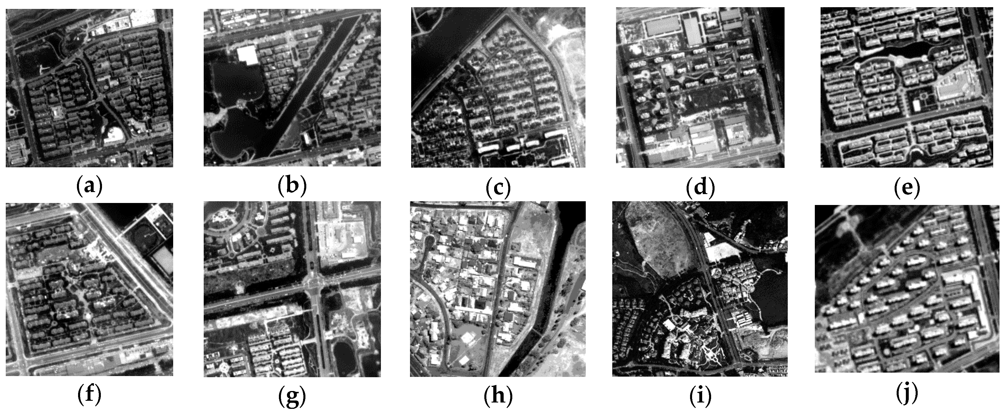
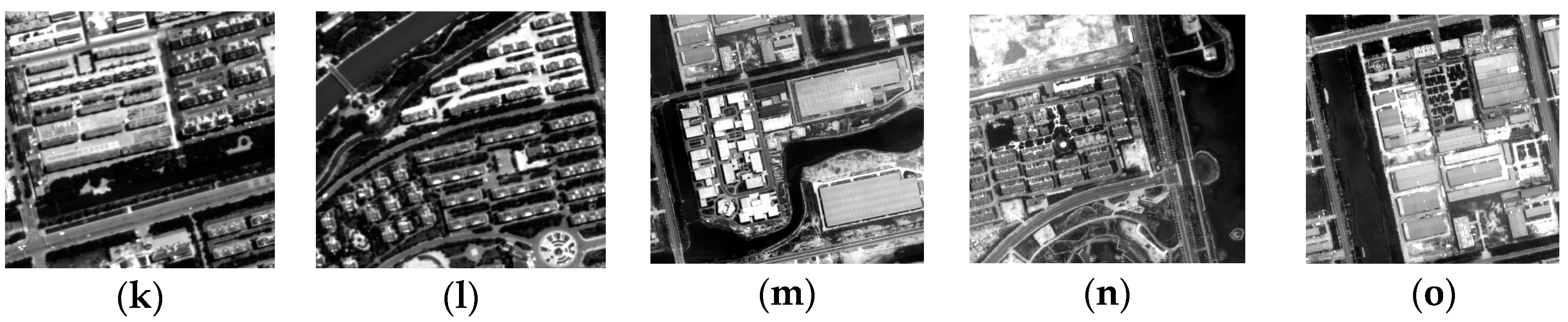
In this section, we analyze the influence of the depth of the network and the convolution kernel. For each category, 1000 labeled pixels were randomly selected from the BJ02 and GF02 images for training and validation. The remaining labeled data served as testing data. 
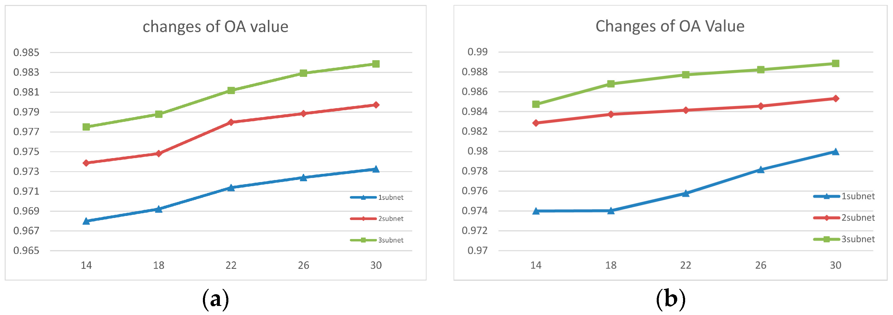
Figure 8a,b illustrate the changing of overall accuracy (OA) for two images under different network structures. Table 2, Table 3, Table 4 and Table 5 list the detailed classification results. The results were the averages of 5 runs of the experiments. We used the most popular OA and kappa as the criteria, in which OA represented the ratio of correct classified pixels to overall pixels and kappa was used for consistency check, serving as a criterion of the classification accuracy as well.
In Figure 8, the vertical axis is the OA value, the horizontal axis is the depth of the convolution kernel. By comparing the results, it is clear that the network structure had a significant influence on the performance of the network.
We found a common trend in the classification accuracy of the BJ02 and GF02 experiments. Firstly, the accuracy of the network classification increased significantly with network depth. In particular, for the network using three subnets and one subnet, the increase in the accuracy of the network was larger than 1%. We theorize that this is because the shallow network focused more on the detailed features but those low-level features were not abstract enough. As the network went deeper, more hierarchical features were extracted. The extracted information contained not only the low-level information focusing on details but also the inherent features that were more discriminative, robust, general and representative of the nature of the ground objects. For the GF02 image, the network comprising two subnets achieved similar results when the kernel depth was small compared with the deeper networks. However, as the kernel depth increased, the difference in accuracy also increased gradually. Although it was not that obvious in the results from the BJ02 experiments, by the joint efforts of the deepest network and the deepest kernel depth (deepest in all compared experimental structures), both images achieved outstanding experimental results. This also proves to some degree that with the combination of increasing depth of network and kernels, the extracted information gets closer to the nature of data, which is the key to distinguishing the pixels from different categories.
In addition to the network depth, the kernel depth also had a significant influence on the capability of the network. The depth of the convolution kernels was the amount of feature maps generated by each convolution. In our experiments, the three-subnet network achieved accuracies higher than 97.7% and 98.4% from the BJ02 and GF02 experiments, respectively, with only 14 convolution kernels. The accuracies were very satisfactory compared with the contrast experiments. In our experiments, when the convolution kernel depth varied from 14 to 30, the accuracy increased with the increasing kernel depth. The increasing kernel depth enable generation of more feature maps, which described the ground objects from different perspectives, making it easier to determine the intrinsic differences among different ground objects and, consequently, achieved better results for ground object classification. Meanwhile, the deepest kernel depth in our experiments was 30, which is not too much to cause redundancy or a large burden for the next layer. Thus, the network performance increasing with increasing kernel depth would not be abnormal. When the depth of the convolution kernel was 30, the overall accuracy was as high as 98.4% and 98.9% under the deepest network structure. From the GF02 and BJ02 experiments, sometimes the influence on the classification accuracy caused by the changes of the kernel depth was stronger in a shallow network than in a deeper network. This might be because in the shallower network, the hierarchical features extracted by the network were insufficient to contribute much to the increase in the classification accuracy of the network. Then, the increasing in diversity of the feature maps compensated for a lack of hierarchical features and made the extracted features more discriminative.
Although employing more subnets and utilizing deeper convolution kernel depths both increased the accuracy in our experiments, it did not mean that we could increase the depth of the network indefinitely. This is because the number of parameters to be trained would increase quickly when the network became wider and deeper. There would be a risk of overfitting when the amount of training samples was small as in our experiments, even though we used some novel approaches to reduce the influence of overfitting. Further, overly many feature maps increased the probability of redundancies and may increase the computation burden in the next layer, making the increase of the classification disproportional to the increase of the feature map numbers. If the increase of accuracy is not obvious while the network training difficulty is significantly increased, then it would make no sense to deepen or widen the network.

4.3.2. Influence of Network Components on Network Performance

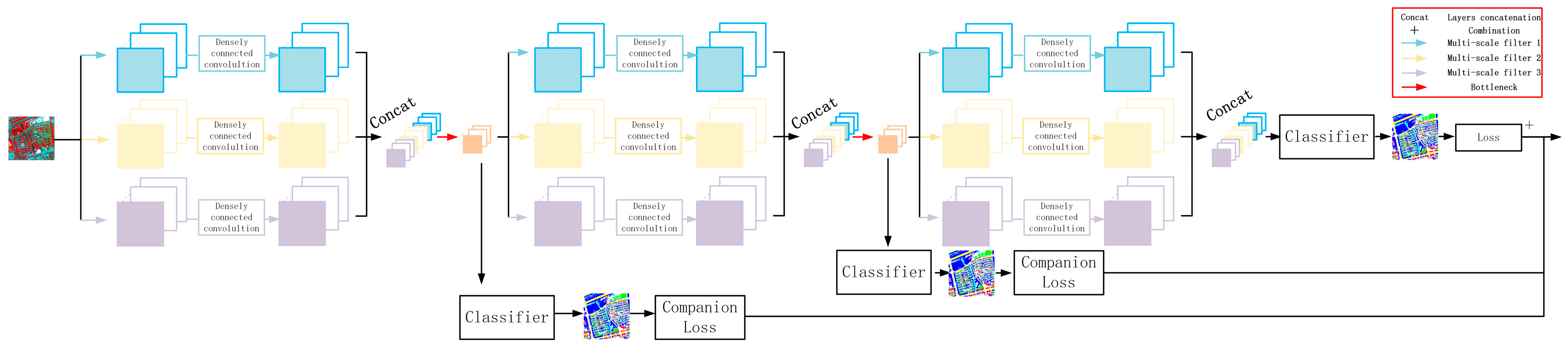
In previous sections, we discussed the reasons why using the dense concatenative convolution, multi-scale filters, as internal classifiers to construct the proposed method theoretically. Here, we use control variables to test the influences of these components, in order to verify the significance and rationality of choosing these components.
In Table 6 and Table 7 we display the OA, KAPPA, user accuracy and producer accuracy of each category.
(1) Influence of the multi-scale filters
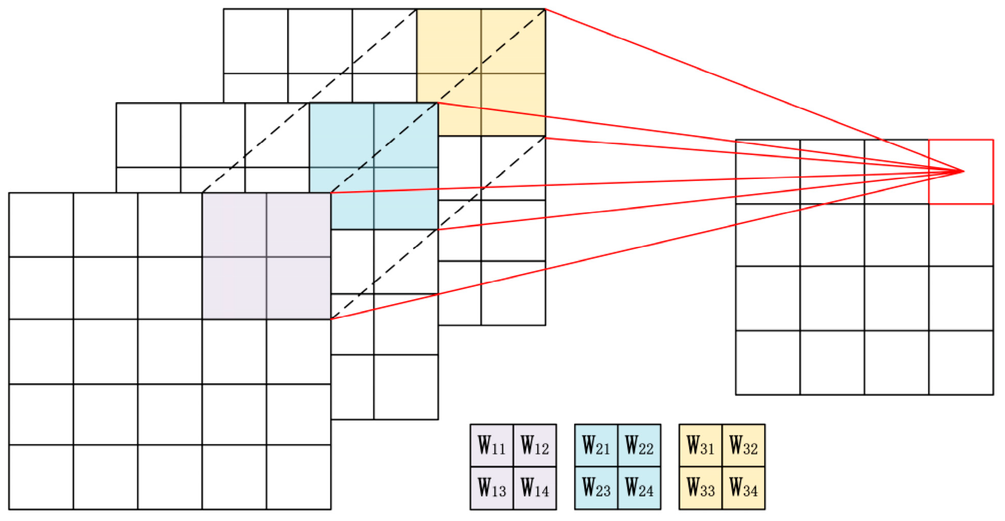
In the proposed method, we used multi-scale filters to get joint spatio-spectral information and diverse local spatial structure information. To determine the influence of multi-scale filters on the network, for both the BJ02 and GF02 experiments, we compared the proposed network with the networks using solely 1 × 1 kernels, 3 × 3 kernels, or 5 × 5 kernels. Those contrast experiments were implemented under the three-subnets network with filter depth of 30 and all the other parameters remained unchanged.
According to the quantitative results, firstly, the accuracy of the network with 1 × 1 kernels was the worst. For the BJ02 experiments, the OA was only 94.5%. Compared with the network using 3 × 3 or 5 × 5 kernels, the difference was more than 3.6%. For the GF02 experiments, OA achieved 98.5% using 5 × 5 kernels while it decreased to 95.6% when the 1 × 1 kernels were used. For both experiments, using combination of three kernels reached highest accuracy. That using 3 × 3 and 5 × 5 filters increased the accuracy significantly, indicates that the spatial structure had a significant influence. The 1 × 1 kernels mainly used spectral correlation information.
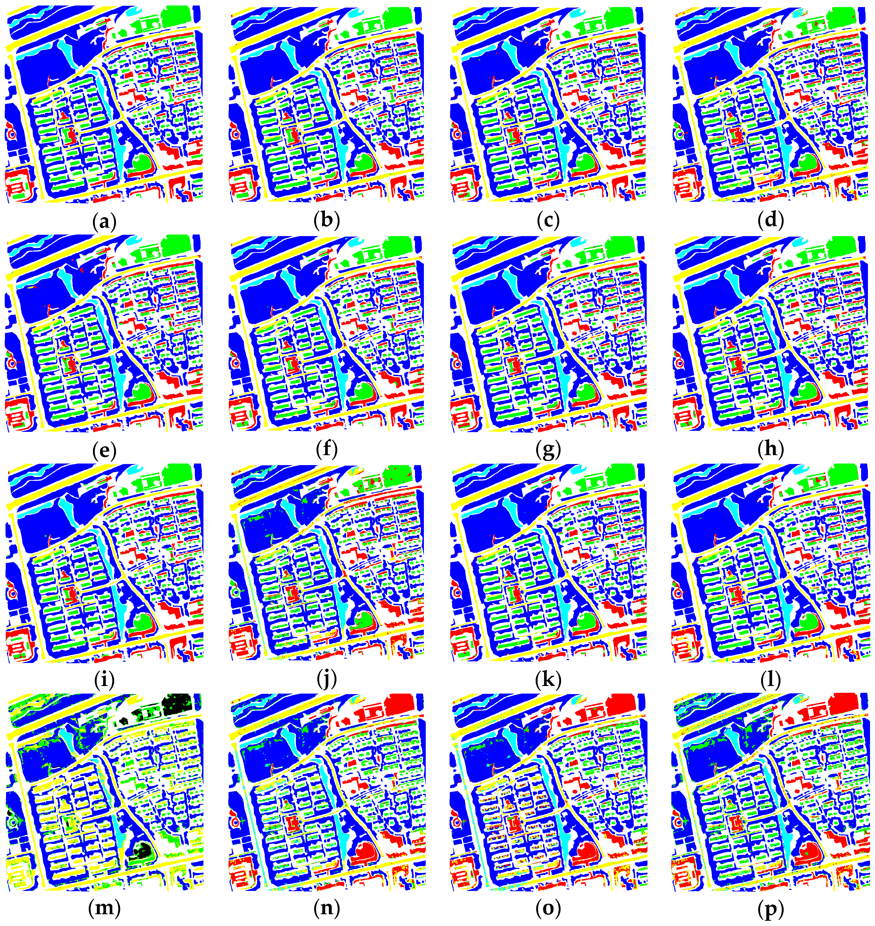
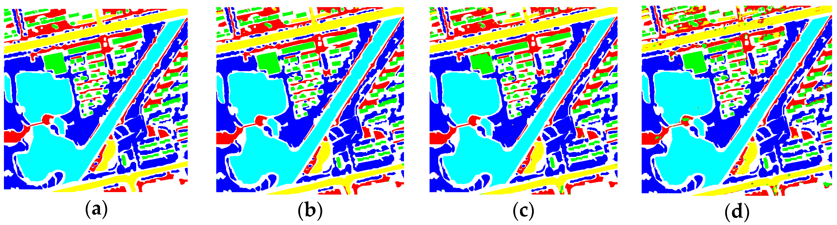
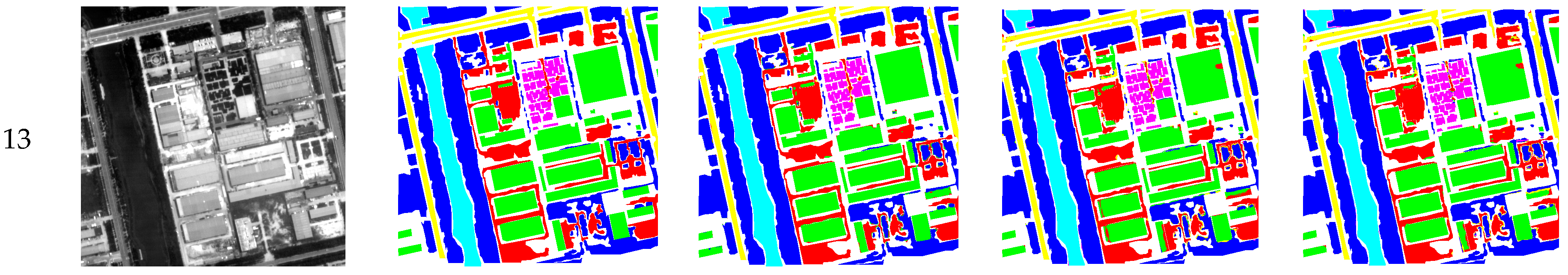
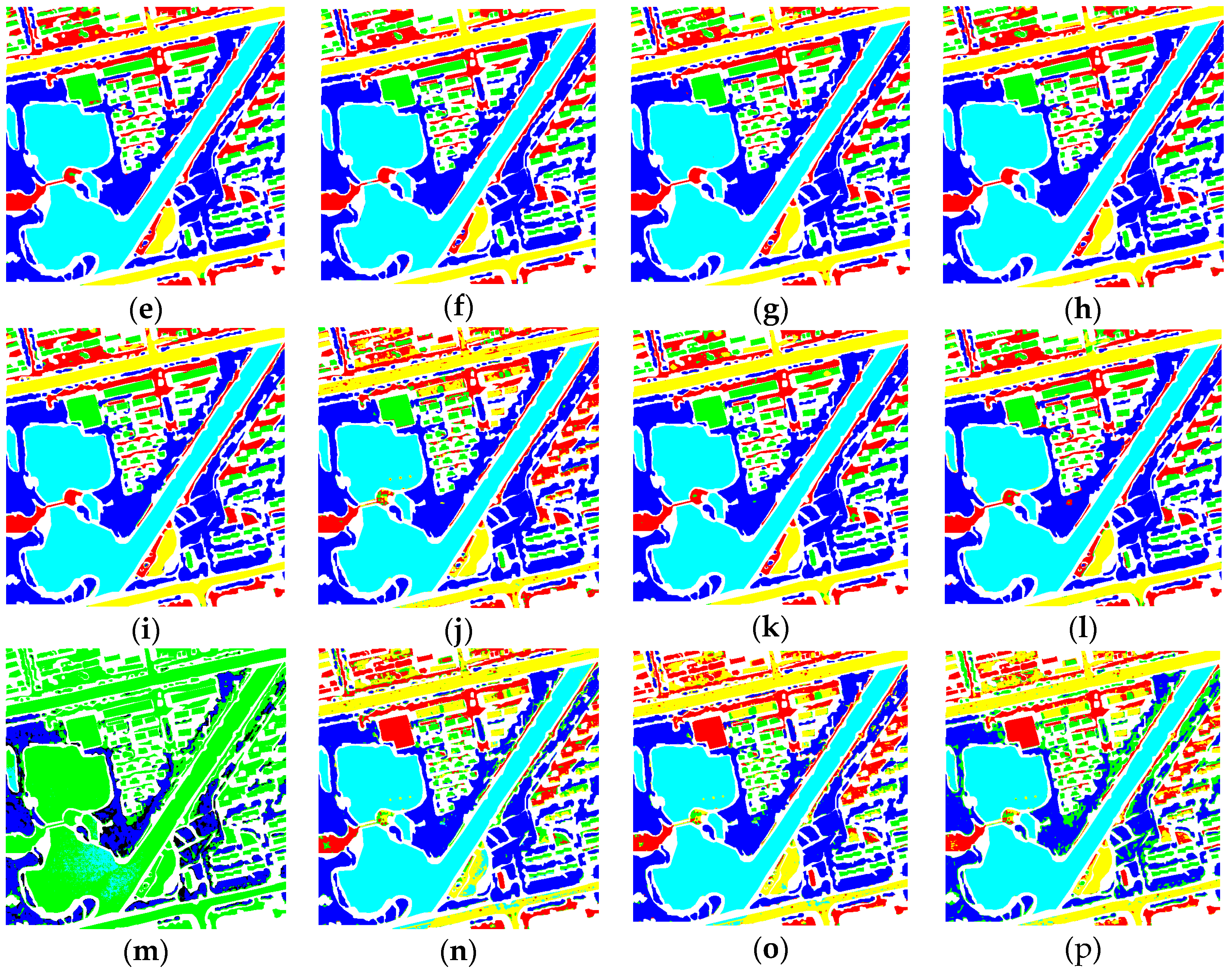
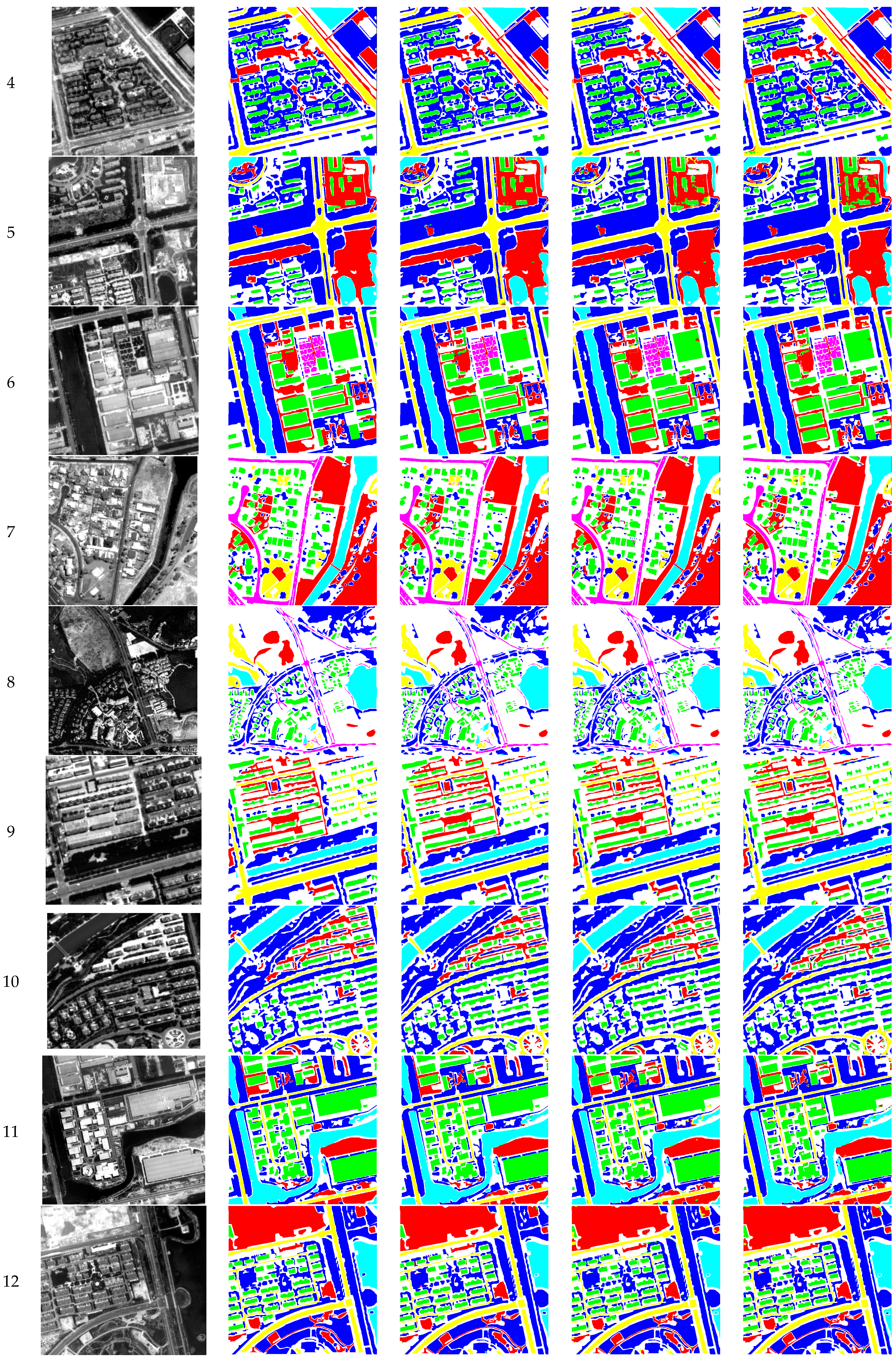
Figure 9 and Figure 10 show the classification results from the BJ02 and GF02 experiments when using three different kinds of filters. Visually speaking, the results generated by using solely 1 × 1 kernels were heavily mottled. The commission errors were serious, no regardless of the inside ground objects or at the boundaries. When using the filters in larger scales, because the spatial structure information was considered, the commission and omission errors obviously decreased. For both the BJ02 and GF02 experiments, the network using 5 × 5 filters achieved the best result and the completeness of the ground objects was greatly improved compared with the network using other filters. Comparing these three methods with the proposed method, although the boundaries of some ground objects were mottled for the proposed method, the misclassifications between bare lands and building, bare land and roads and buildings and roads that were found in the others were significantly reduced and the results were more similar to the labeled images. We theorize that it is closely related to the joint of spatio-spectral information and the combination of diverse local structures. However, in all the methods, roads, bare lands and buildings were most likely to be misclassified compared with others. This might be because these ground objects used similar building materials; hence, those ground objects possessed similar spectral information and consequently resulted in the decrease in the classification accuracy.
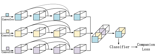
(2) Influence of the internal classifier on the network
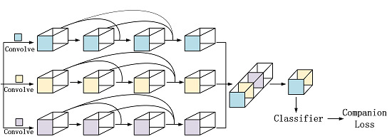
The purpose of using internal classifiers is to increase the transparency of the hidden layers. Inputting the feature maps generated by the hidden layers directly into the internal classifier to get the companion loss and then combining the companion loss with the loss from the final layer makes the features from hidden layers more discriminative, enhancing the robustness and reducing the information redundancies.
OA and KAPPA changed significantly when the network was with or without the internal classifiers. For the BJ02 experiments, OA decreased about 0.6% and KAPPA decreased 1%. With the internal classifiers removed, although the boundaries were well maintained, the completeness of the ground objects was not as good as that from using internal classifiers. There were obvious commission errors inside the ground objects. Some of them were in dots, some of them were in large areas, for example the bare lands and buildings inside the trees.
For the GF02 experiments, OA decreased 0.5% to 98.4%. KAPPA decreased 0.7% to 97.8%. From Figure 9 clearly shows that, without the internal classifier the misclassifications between buildings and bare lands and between buildings and roads are more obvious, while the proposed methods preserved the completeness of the buildings better.
The decreased accuracy indicates that when internal classifiers are removed, the features used for the classification are not that discriminative and because the internal classifiers also had some effect on strengthening the gradients, when using the network with the internal classifiers, they could back propagate stronger feedback on gradients from different layers. Therefore, when those companion classifiers were removed, the accuracy decreased distinctly.
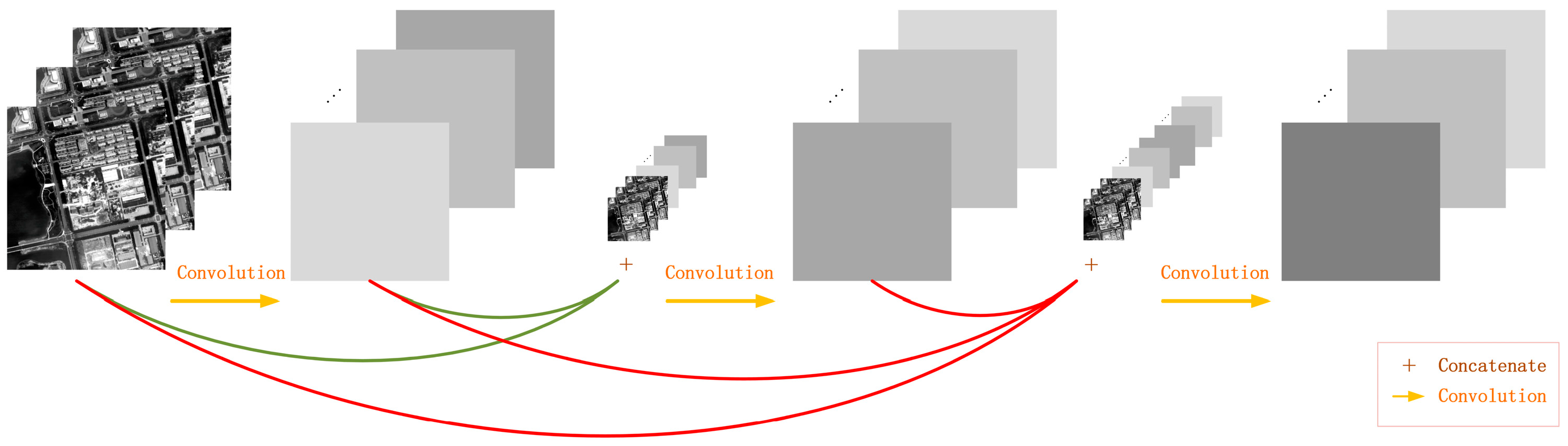
(3) Influence of the DenseNet on the network
We removed the densely connected convolution and utilized normal convolution instead. When the dense concatenation was removed, for two experiments, both of their OAs decreased by about 1% and KAPPAs decreased by about 1.5%. For the BJ02 experiments, according to the classification result images in Figure 9, some pixels inside buildings or roads were misclassified as other ground objects obviously, for instance, the buildings on the right and the roads in the middle. For the GF02 experiments, from Figure 10, some pixels inside the bare lands were obviously misclassified as roads close to the edges of the GF image.
This proves that DenseNet can make use of the advantages brought by the depth of the deep network, that deeper network possesses stronger expression ability. Because the dense concatenation reutilized the feature maps, the connections between the layers close to the input layers and output layers were shorter, which alleviated the problems harming the network performance, such as gradient disappearance, brought by the deeper network and made deepening the network more sensible.

4.3.3. Contrast Experiments with Other Networks

To test the effectiveness and practicability of the proposed method, we introduced five kinds of networks similar to the proposed method: DNN [47], URDNN [48], contextual deep CNN [17], two-stream neural network [26] and SAE + SVM [
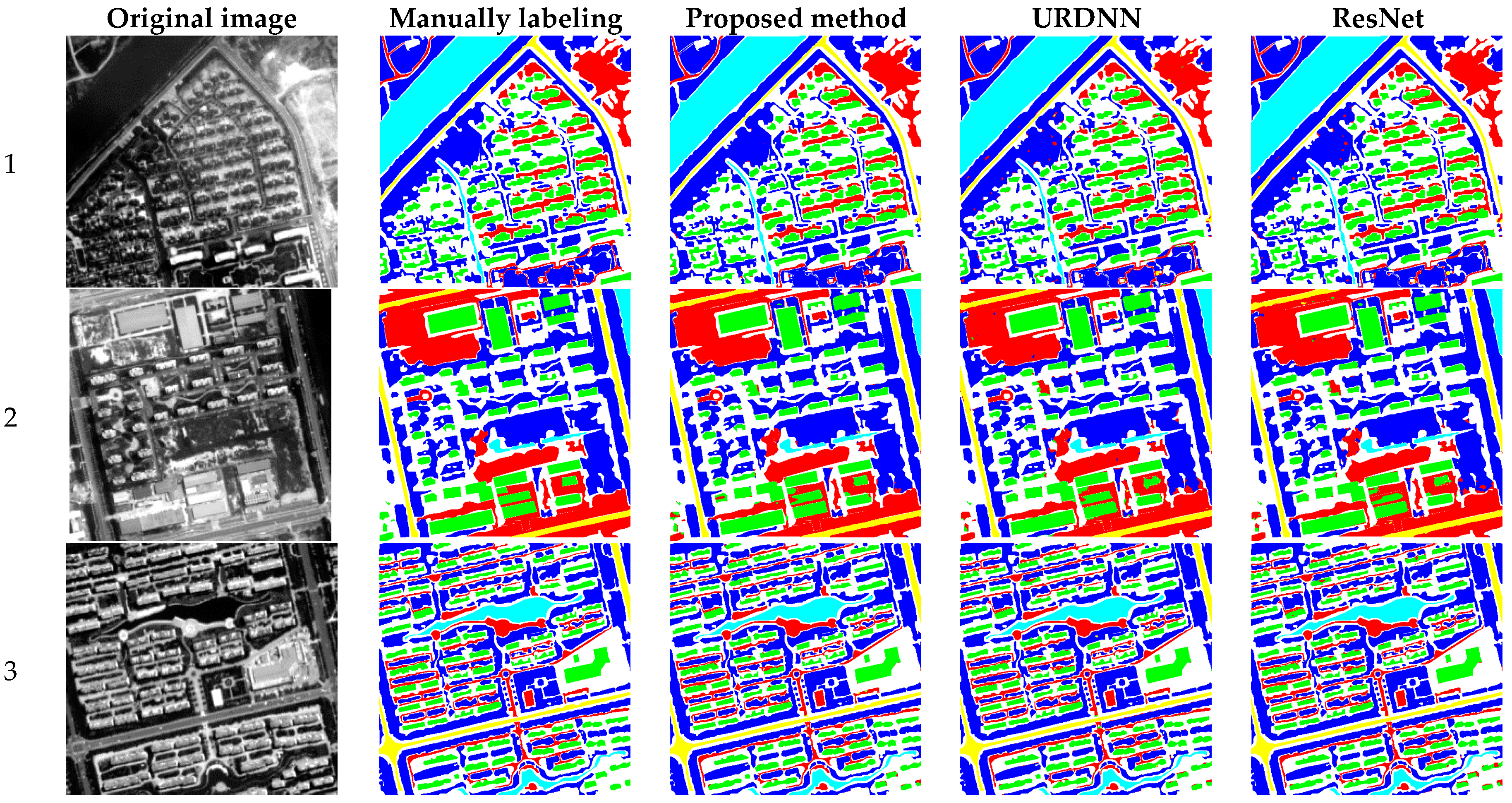
49]. DNN uses deconvolution to realize an end-to-end, pixel-to-pixel classification. It has also become a prevalent method for per-pixel classification recently. URDNN utilizes the unsupervised network to support and control the supervised classification, using both labeled and unlabeled pixels to alleviate the overfitting problems caused by a small number of samples. We revised the original URDNN and added feature concatenation in the last layer to make it more comparable with the proposed method. Contextual deep CNN and two-stream network all rely on ResNet to reduce the problems like gradient disappearance and overfitting, which were coherent with our aim. SAE + SVM used the unsupervised method to extract features and then utilized SVM as the classifier for the classification. All the methods mentioned above were neural network algorithms. Besides neural network based methods, we also introduced some simple classification methods without using neural network for comparison, which were parallel piped, minimum distance, mahalanobis distance and maximum likelihood methods.
Table 6 and Table 7 and Figure 9 and Figure 10 illustrate the results in detail.
For the BJ02 experiment, the two networks utilizing ResNet achieved accuracies of 97.6% and 97.7%, respectively. The boundaries of the ground objects were well retained but there were some misclassifications in some small roads and inside the buildings and trees. Contextual deep CNN mainly misclassified buildings as bare lands, while the two-stream network performed well in the classification between buildings and bare lands but was prone to mix buildings with the roads. Those ground objects were similar in their spectral information. URDNN does not adopt ResNet to reduce gradient disappearance and overfitting but it utilizes the feature extraction of the unlabeled data and performed well with the classification accuracy of 97.7%. The DNN performed relatively poorly compared with the aforementioned methods. In addition to the previously mentioned misclassification, it also tended to misclassify bare lands as roads and resulted in lower classification accuracy. SAE + SVM was the only method solely relying on the unsupervised feature extraction but it performed worst.
The results from simple classification methods were much worse than what we have achieved using proposed neural network method, no matter from accuracy aspect or visual effect aspect. Some simple classification methods could do well on classifying simple ground object categories, such as water and tree. However, they seemed not to be suitable for classifying some complex or confusing categories, like bare land, building and road, which caused serious misclassification. From computational cost aspect, using such simple classification methods would be more efficient. It just needed several seconds to do the classification while we required about 4 h to train our network. But this efficiency could not compensate their deficiency in VHRRS image per-pixel classification accuracy.
Compared with these contrast methods, the proposed method achieved the competitive results, with OA of 98.4% and kappa of 97.3%. From Figure 9, although some boundaries of ground objects were not well preserved, for instance, some building boundaries, the errors inside the ground objects were greatly reduced. The ground objects extracted by the proposed method were more complete. Although there were still misclassifications between buildings and bare lands and between bare lands and roads, the classification result was getting more similar to the labeled ground truth.
For the GF02 experiment, the proposed method achieved an OA as high as 98.9%, which is about 0.7% higher compared with other contrast methods. ResNet-based contextual deep CNN achieved the best result in five contrast methods. Although the improved URDNN did not use ResNet, its OA were all over 98.1%. However, compared with the proposed method, these contrast methods did not preserve the completeness of the ground objects well enough, especially inside the buildings and bare lands. In addition, there are more commission errors on the boundaries of the buildings and the roads. The SAE + SVM method performed poorly in the GF02 experiment as well, the bare lands and the roads were heavily mixed, so the results looked mottled. The simple classification methods without using neural network also behaved worse compared with proposed method, especially in some confusing categories, like building and bare land.
The proposed network was not advantageous in terms of training and classification time because it contains many convolutions that are very time-consuming, especially for those 5 × 5 convolutions. Although we reduced the depth of filters to control it but time training time for the whole network was about 4 h when the subnet number was three and filter depth was 30, using the Quadro K620 graphic card. In the testing, the time to generate the classification result was 1.2 s, which was not too long.

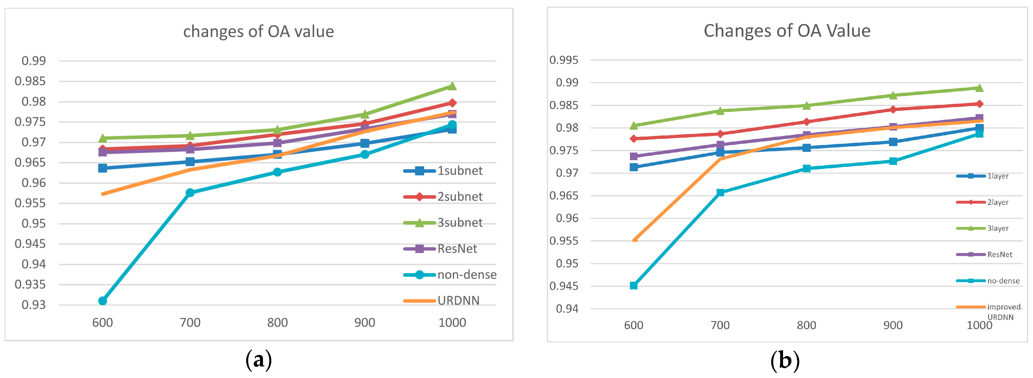
4.3.4. Influence of Training Data Size on Network Performance

Because of the complexity of the deep network and the large number of parameters to be trained, when the labeled training data were few, overfitting tended to happen and resulted in the decrease in the classification accuracy. The network performance was not in proportion to the network depth. In the field of per-pixel classification of VHRRS, it is hard to acquire the labeled data. Therefore, it is challenging to make the model more robust with a small number of samples. For the BJ02 and GF02 experiments, we chose 600, 700, 800, 900 and 1000 pixels for each category as training samples. The changes of the overall accuracy are shown in Figure 11, in which ResNet represents the contextual deep CNN and non-dense represented the proposed method with the densely connected convolution removed. For the BJ02 and GF02 experiments, the decease of the amount of training samples generated some similar trends.
Firstly, when using 600 training samples, the proposed method with three subnets achieved the best results. In the BJ02 experiments, the OA reached 97%; and in the GF02 experiments, OA reached 98%, both of which were satisfactory. Secondly, we could see that although the accuracies of all the methods decreased when the amount of training sample was reduced, when using the URDNN and the proposed method with densely connected removed, the speed and range of the decease were quicker and larger. When using DenseNet and ResNet, the changes were relatively steady. Especially for the contextual deep CNN, the changes were quite small, which proved that its model is quite robust. Our proposed method changed more obviously when using 3 subnets than using 2 subnets or one subnet, this was because the 3-subnets network was more complicated and had more parameters. Although it employed DenseNet and internal classifiers to reduce the gradient disappearance and overfitting, it was prone to be influenced by the number of samples than the simpler networks. However, it still achieved satisfactory results with a small number of samples.
When the densely connected convolution was removed, the network classification accuracy decreased rapidly as the number of training samples was reduced, which also proves that the increase in the transparency of the hidden layers was beneficial to counter the overfitting problem. DenseNet was useful for the network to extract more discriminative features and made the models more appropriate for the training and classification in the circumstance of small number of training samples.
In general, the proposed method performed consistently when the training data were reduced. It was suitable for the scenario of the RHRRS classification where the labeled training data were lacking. It could strengthen the capability of data extraction of the network, enabling the network to achieve better results when the number of samples is small.

4.3.5. More Experiments and Verifications

To test the validity and feasibility of the proposed method, in addition to the aforementioned two scene images, we also applied the proposed method to another thirteen images. The classification accuracies are given in Table 8. For each category, the producer’s accuracy and user’s accuracy were calculated and are separated by “/”. In consideration of the space and the performance of different contrast methods in Section 4.3.3, we chose two methods as contrast methods: ResNet and improved URDNN. Compared with these two methods, in most circumstances the proposed method performed best and obviously achieved the leading accuracies. Figure 12 shows images of the classification results. The proposed method performed better than the contrast methods regarding the completeness and the preservation of the boundaries for each ground category.

5. Conclusions

This paper proposed a double reinforced deep learning neural network from two perspectives, deepening and widening of the network, with the aim of building a more effective network for very high resolution remote sensing per-pixel classification. The proposed method utilizes densely connected convolution from the DenseNet concept and internal classifiers to make a deeper neural network. It takes advantage of DenseNet to achieve feature maps reuse and densely connected convolution helps it to achieve better feature extraction using smaller filter depth and to decrease the redundancy. Further, it makes shorter connections from input and output layers, which strengthens the gradients and reduces the negative effects on network performance brought by gradient disappearance. Internal classifiers are designed not only to enhance the features and gradients but also to increase the transparency of hidden layers, making extracted features from hidden layers more objective and targeted, in order to reinforce its level of discrimination and reduce the redundancy. In addition to width, the proposed method also enhances feature extraction capability from widening of the network. Multi-scale filters are also involved, with 1 × 1 filters helping to extract spectral coherence and 3 × 3 and 5 × 5 filters designed to extract diverse local spatial structures. Thus, enabling extraction of features from different views and making the range of information extraction broader and more abundant. To better fuse the network deepening and widening strategy, the “network in network” concept was utilized. It helps the double reinforced deep learning neural network to go smoothly and improves the network’s expression ability as well, which enables it to deal with more complicated situations and makes model performance better.
During the experiments, the influence on network performance of network structure parameters (network depth, filter depth, etc.) was examined. It was found that the network depth and more generated feature maps may benefit network performance. Further, the proposed method was compared with densely connected convolution, multi-scale filters and internal classifiers removed. The better results obtained by the proposed method prove the importance and rationality of these components.
The proposed method was also tested on ten images from the BJ02, GF02, geoeye and quickbird satellites. It outperformed the compared methods and achieved competitive and leading classification accuracies, illustrating its effectiveness. Meanwhile, when faced with decreasing amounts of labeled training samples, it behaved well, proving that the network may be suitable for VHRRS per-pixel classification, in which field, obtaining labeled training data is very expensive and time-consuming.
There still exist some limitations for this proposed method. First of all, our proposed method is a kind of complex deep network containing a lot of convolution, pooling, non-linearity and concatenating layers and utilizing multi-scale kernels for convolution. During the training of the network, the forward and backward propagations contain a lot of floating-point calculation and so on, which is considered to be complex and time-consuming. Though if better CPU and GPU are utilized, the training time can be shortened, we will try to shorten the time by improving the model in the future work. Secondly, the amount of network parameters will increase sharply when network going deeper. If the amount of labeled training samples cannot meet the demand for training a deep model, overfitting tends to happen and results in the decrease in the classification performance. Even though we focus on building a more robust deep neural network using less labeled training pixels, to simulate the reality that labeled ground truth is very rare and expensive in very high resolution remote sensing image per pixel classification field and we have used some novel approaches to reduce the influence of overfitting, it does not mean we can contain subnets as many as we wish. If we provide extremely small number of labeled pixels or adopt too many subnets, the method may fail. But the extreme limits vary from case to case, so here we just give such examples to reveal some possible situations in which the method may fail. How to decrease the negative effects from those factors will still be studied in our future work.

Author Contributions

Y.T. and M.X. conceived and conducted the experiments, as well as performing the data analysis; and Z.L. helped labeling the ground truth and conducted some comparison experiments. Y.Z. provided advices and helped revising the manuscript. Y.T. wrote the paper.

Acknowledgments

The authors would like to thank the editors and anonymous reviewers for their valuable comments, which helped us improve this work. This work was supported by National Natural Science Foundation of China under Grant Nos. 41622107, 41771385 and 41371344. GaoFen-2 data are provided by CRESDA and Beijing-2 data are provided by Twenty First Century Aerospace Technology. In addition, the authors would like to give our special thanks to Ming Cong and Zhiye Wang for their moral support.

Conflicts of Interest

The authors declare no conflict of interest.

References

  1. Huang, Z.; Cheng, G.; Wang, H.; Li, H.; Shi, L.; Pan, C. Building extraction from multi-source remote sensing images via deep deconvolution neural networks. In Proceedings of the IEEE International Geoscience and Remote Sensing Symposium (IGARSS), Beijing, China, 10–15 July 2016; pp. 1835–1838. [Google Scholar]
  2. Wei, Y.; Wang, Z.; Xu, M. Road structure refined CNN for road extraction in aerial image. IEEE Geosci. Remote Sens. Lett. 2017, 14, 709–713. [Google Scholar] [CrossRef]
  3. Hwang, J.-J.; Liu, T.-L. Pixel-wise deep learning for contour detection. arXiv, 2015; arXiv:1504.01989. [Google Scholar]
  4. Zhao, W.; Du, S. Spectral–spatial feature extraction for hyperspectral image classification: A dimension reduction and deep learning approach. IEEE Trans. Geosci. Remote Sens. 2016, 54, 4544–4554. [Google Scholar] [CrossRef]
  5. Reis, S.; Tasdemir, K. Identification of hazelnut fields using spectral and Gabor textural features. ISPRS J. Photogramm. Remote Sens. 2011, 66, 652–661. [Google Scholar] [CrossRef]
  6. Wang, T.; Zhang, H.; Lin, H.; Fang, C. Textural–spectral feature-based species classification of mangroves in Mai Po Nature Reserve from Worldview-3 imagery. Remote Sens. 2016, 8, 24. [Google Scholar] [CrossRef]
  7. Yu, H.; Yang, W.; Xia, G.-S.; Liu, G. A color-texture-structure descriptor for high-resolution satellite image classification. Remote Sens. 2016, 8, 259. [Google Scholar] [CrossRef]
  8. Huang, L.; Chen, C.; Li, W.; Du, Q. Remote sensing image scene classification using multi-scale completed local binary patterns and Fisher vectors. Remote Sens. 2016, 8, 483. [Google Scholar] [CrossRef]
  9. Cheng, G.; Han, J.; Guo, L.; Liu, Z.; Bu, S.; Ren, J. Effective and efficient midlevel visual elements-oriented land-use classification using VHR remote sensing images. IEEE Trans. Geosci. Remote Sens. 2015, 53, 4238–4249. [Google Scholar] [CrossRef]
  10. Chaib, S.; Liu, H.; Gu, Y.; Yao, H. Deep feature fusion for VHR remote sensing scene classification. IEEE Trans. Geosci. Remote Sens. 2017, 55, 4775–4784. [Google Scholar] [CrossRef]
  11. Zhang, F.; Du, B.; Zhang, L. Scene classification via a gradient boosting random convolutional network framework. IEEE Trans. Geosci. Remote Sens. 2016, 54, 1793–1802. [Google Scholar] [CrossRef]
  12. Li, E.; Xia, J.; Du, P.; Lin, C.; Samat, A. Integrating multilayer features of convolutional neural networks for remote sensing scene classification. IEEE Trans. Geosci. Remote Sens. 2017, 55, 5653–5665. [Google Scholar] [CrossRef]
  13. Bazi, Y.; Melgani, F. Convolutional SVM Networks for Object Detection in UAV Imagery. IEEE Trans. Geosci. Remote Sens. 2018, 1–12. [Google Scholar] [CrossRef]
  14. He, K.; Zhang, X.; Ren, S.; Sun, J. Deep residual learning for image recognition. In Proceedings of the IEEE Conference on Computer Vision and Pattern Recognition, Fontainebleau Resort, Miami, FL, USA, 26 June–1 July 2016; pp. 770–778. [Google Scholar]
  15. Pohlen, T.; Hermans, A.; Mathias, M.; Leibe, B. Full-Resolution Residual Networks for Semantic Segmentation in Street Scenes. arXiv, 2016; arXiv:1611.08323. [Google Scholar]
  16. Mou, L.; Ghamisi, P.; Zhu, X.X. Unsupervised spectral-spatial feature learning via deep residual conv-deconv network for hyperspectral image classification. IEEE Trans. Geosci. Remote Sens. 2018, 56, 391–406. [Google Scholar] [CrossRef]
  17. Lee, H.; Kwon, H. Going deeper with contextual CNN for hyperspectral image classification. IEEE Trans. Image Process. 2017, 26, 4843–4855. [Google Scholar] [CrossRef] [PubMed]
  18. Huang, G.; Liu, Z.; Weinberger, K.Q.; van der Maaten, L. Densely connected convolutional networks. In Proceedings of the IEEE Conference on Computer Vision and Pattern Recognition, Honolulu, HI, USA, 21–26 July 2017; Volume 1, p. 3. [Google Scholar]
  19. Huang, G.; Sun, Y.; Liu, Z.; Sedra, D.; Weinberger, K.Q. Deep networks with stochastic depth. In Proceedings of the European Conference on Computer Vision (ECCV), Amsterdam, The Netherlands, 6–12 September 2016; pp. 646–661. [Google Scholar]
  20. Springenberg, J.T.; Dosovitskiy, A.; Brox, T.; Riedmiller, M. Striving for simplicity: The all convolutional net. arXiv, 2014; arXiv:1412.6806. [Google Scholar]
  21. Lee, C.Y.; Xie, S.; Gallagher, P.; Zhang, Z.; Tu, Z. Deeply-supervised nets. In Proceedings of the Artificial Intelligence and Statistics, San Diego, CA, USA, 9–12 May 2015; pp. 562–570. [Google Scholar]
  22. Krizhevsky, A.; Sutskever, I.; Hinton, G.E. ImageNet classification with deep convolutional neural networks. In Proceedings of the Advances in Neural Information Processing Systems (NIPS), Lake Tahoe, NV, USA, 3–8 December 2012; pp. 1097–1105. [Google Scholar]
  23. Simonyan, K.; Zisserman, A. Very deep convolutional networks for large-scale image recognition. arXiv, 2014; arXiv:1409.1556. [Google Scholar]
  24. Lin, M.; Chen, Q.; Yan, S. Network in network. arXiv, 2013; arXiv:1312.4400. [Google Scholar]
  25. Soriano, A.; Vergara, L.; Ahmed, B.; Salazar, A. Fusion of scores in a detection context based on Alpha integration. Neural Comput. 2015, 27, 1983–2010. [Google Scholar] [CrossRef] [PubMed]
  26. Tao, Y.; Xu, M.; Zhong, Y.; Cheng, Y. GAN-Assisted Two-Stream Neural Network for High-Resolution Remote Sensing Image Classification. Remote Sens. 2017, 9, 1328. [Google Scholar] [CrossRef]
  27. Hao, S.; Wang, W.; Ye, Y.; Nie, T.; Bruzzone, L. Two-Stream Deep Architecture for Hyperspectral Image Classification. IEEE Trans. Geosci. Remote Sens. 2017, 56, 2349–2361. [Google Scholar] [CrossRef]
  28. Xu, X.; Li, W.; Ran, Q.; Du, Q.; Gao, L.; Zhang, B. Multisource remote sensing data classification based on convolutional neural network. IEEE Trans. Geosci. Remote Sens. 2018, 56, 937–949. [Google Scholar] [CrossRef]
  29. Hu, J.; Mou, L.; Schmitt, A.; Zhu, X.X. FusioNet: A two-stream convolutional neural network for urban scene classification using PolSAR and hyperspectral data. In Proceedings of the Urban Remote Sensing Event (JURSE), Dubai, UAE, 6–8 March 2017; pp. 1–4. [Google Scholar]
  30. Han, X.; Zhong, Y.; Cao, L.; Zhang, L. Pre-Trained AlexNet Architecture with Pyramid Pooling and Supervision for High Spatial Resolution Remote Sensing Image Scene Classification. Remote Sens. 2017, 9, 848. [Google Scholar] [CrossRef]
  31. Szegedy, C.; Liu, W.; Jia, Y.; Sermanet, P.; Reed, S.; Anguelov, D.; Erhan, D.; Vanhoucke, V.; Rabinovich, A. Going deeper with convolutions. In Proceedings of the IEEE International Conference on Computer Vision and Pattern Recognition, Boston, MA, USA, 7–12 June 2015; pp. 1–9. [Google Scholar]
  32. Jia, Y.; Shelhamer, E.; Donahue, J.; Karayev, S.; Long, J.; Girshick, R.; Guadarrama, S.; Darrell, T. Caffe: Convolutional architecture for fast feature embedding. In Proceedings of the 22nd ACM International Conference on Multimedia (MM), Orlando, FL, USA, 3–7 November 2014; pp. 675–678. [Google Scholar]
  33. Cheng, G.; Zhou, P.; Han, J. Learning rotation-invariant convolutional neural networks for object detection in VHR optical remote sensing images. IEEE Trans. Geosci. Remote Sens. 2016, 54, 7405–7415. [Google Scholar] [CrossRef]
  34. Liang, H.; Lin, X.; Zhang, Q.; Kang, X. Recognition of spoofed voice using convolutional neural networks. In Proceedings of the IEEE Global Conference on Signal and Information Processing (GlobalSIP), Montreal, QC, Canada, 14–16 November 2017; pp. 293–297. [Google Scholar]
  35. Salehinejad, H.; Barfett, J.; Aarabi, P.; Valaee, S.; Colak, E.; Gray, B.; Dowdell, T. A Convolutional Neural Network for Search Term Detection. arXiv, 2017; arXiv:1708.02238. [Google Scholar]
  36. Romero, A.; Gatta, C.; Camps-Valls, G. Unsupervised deep feature extraction for remote sensing image classification. IEEE Trans. Geosci. Remote Sens. 2016, 54, 1349–1362. [Google Scholar] [CrossRef]
  37. Chen, Y.; Jiang, H.; Li, C.; Jia, X.; Ghamisi, P. Deep feature extraction and classification of hyperspectral images based on convolutional neural networks. IEEE Trans. Geosci. Remote Sens. 2016, 54, 6232–6251. [Google Scholar] [CrossRef]
  38. Long, Y.; Gong, Y.; Xiao, Z.; Liu, Q. Accurate object localization in remote sensing images based on convolutional neural networks. IEEE Trans. Geosci. Remote Sens. 2017, 55, 2486–2498. [Google Scholar] [CrossRef]
  39. Liu, Y.; Liu, Y.; Ding, L. Scene Classification Based on Two-Stage Deep Feature Fusion. IEEE Geosci. Remote Sens. Lett. 2018, 15, 183–186. [Google Scholar] [CrossRef]
  40. Yu, Y.; Gong, Z.; Wang, C.; Zhong, P. An Unsupervised Convolutional Feature Fusion Network for Deep Representation of Remote Sensing Images. IEEE Geosci. Remote Sens. Lett. 2018, 15, 23–27. [Google Scholar] [CrossRef]
  41. Song, W.; Li, S.; Fang, L.; Lu, T. Hyperspectral Image Classification with Deep Feature Fusion Network. IEEE Trans. Geosci. Remote Sens. 2018, 1–12. [Google Scholar] [CrossRef]
  42. Maggiori, E.; Tarabalka, Y.; Charpiat, G.; Alliez, P. Convolutional neural networks for large-scale remote-sensing image classification. IEEE Trans. Geosci. Remote Sens. 2017, 55, 645–657. [Google Scholar] [CrossRef]
  43. Kampffmeyer, M.; Salberg, A.-B.; Jenssen, R. Semantic segmentation of small objects and modeling of uncertainty in urban remote sensing images using deep convolutional neural networks. In Proceedings of the IEEE Computer Vision and Pattern Recognition Workshops (CVPRW), Las Vegas, NV, USA, 26 June–1 July 2016; pp. 680–688. [Google Scholar]
  44. Yu, F.; Koltun, V. Multi-scale context aggregation by dilated convolutions. arXiv, 2015; arXiv:1511.07122. [Google Scholar]
  45. Szegedy, C.; Vanhoucke, V.; Ioffe, S.; Shlens, J.; Wojna, Z. Rethinking the inception architecture for computer vision. In Proceedings of the IEEE Conference on Computer Vision and Pattern Recognition (CVPR), Las Vegas, NV, USA, 27–30 June 2016; pp. 2818–2826. [Google Scholar]
  46. Glorot, X.; Bengio, Y. Understanding the difficulty of training deep feedforward neural networks. J. Mach. Learn. Res. 2010, 9, 249–256. [Google Scholar]
  47. Volpi, M.; Tuia, D. Dense semantic labeling of subdecimeter resolution images with convolutional neural networks. IEEE Trans. Geosci. Remote Sens. 2017, 55, 881–893. [Google Scholar] [CrossRef]
  48. Tao, Y.; Xu, M.; Zhang, F.; Du, B.; Zhang, L. Unsupervised-Restricted Deconvolutional Neural Network for Very High Resolution Remote-Sensing Image Classification. IEEE Trans. Geosci. Remote Sens. 2017, 55, 6805–6823. [Google Scholar] [CrossRef]
  49. Chen, Y.; Lin, Z.; Zhao, X.; Wang, G.; Gu, Y. Deep learning-based classification of hyperspectral data. IEEE J. Sel. Top. Appl. Earth Obs. Remote Sens. 2014, 7, 2094–2107. [Google Scholar] [CrossRef]
Figure 1. Illustration of convolution.
Remotesensing 10 00779 g001
Figure 2. Flowchart of a traditional convolutional neural network (CNN).
Remotesensing 10 00779 g002
Figure 3. Flowchart of the proposed “network in network” method.
Remotesensing 10 00779 g003
Figure 4. Operation of densely connected convolution.
Remotesensing 10 00779 g004
Figure 5. Dilated convolution.
Remotesensing 10 00779 g005
Figure 6. Structure of a subnetwork in the proposed network method.
Remotesensing 10 00779 g006
Figure 7. The ten experimental images: (a,c,f,jl) are from the BJ02 satellite; (b,d,e,g,mo) are from the GF02 satellite; (h,i) are from the geoeye and quickbird satellites, respectively.
Remotesensing 10 00779 g007aRemotesensing 10 00779 g007b
Figure 8. (a,b) display the overall accuracy acquired from the BJ02 and GF02 images, respectively, based on different network structures.
Remotesensing 10 00779 g008
Figure 9. BJ02 classification results from (a) manually labeled reference data, (b) proposed method, (c) internal classifier-removed, (d) method using 1 × 1 kernel, (e) method using 3 × 3 kernel, (f) method using 5 × 5 kernel, (g) ResNet-based method using contextual deep CNN, (h) method without densely connected convolution, (i) improved URDNN, (j) SCAE + SVM, (k) two-stream network, (l) deconvolution, (m) parallelepiped, (n) minimum distance, (o) Mahalanobis distance and (p) maximum likelihood.
Remotesensing 10 00779 g009
Figure 10. GF02 classification results from (a) manually labeled reference data, (b) proposed method, (c) internal classifier-removed, (d) method using 1 × 1 kernel, (e) method using 3 × 3 kernel, (f) method using 5 × 5 kernel, (g) ResNet-based method using contextual deep CNN, (h) method without densely connected convolution, (i) improved URDNN, (j) SCAE + SVM, (k) two-stream network, (l) deconvolution, (m) parallelepiped, (n) minimum distance, (o) Mahalanobis distance and (p) maximum likelihood.
Remotesensing 10 00779 g010aRemotesensing 10 00779 g010b
Figure 11. (a,b) are changes of OA values for the BJ02 experiments and GF02 experiments, respectively, with the amount of training data decreasing.
Remotesensing 10 00779 g011
Figure 12. Classification images for extra eight images.
Remotesensing 10 00779 g012aRemotesensing 10 00779 g012bRemotesensing 10 00779 g012c
Table 1. Reference data information for BJ02 and GF02 images.
BJSize 800 × 800GFSize 570 × 570
No.CategoryMark ColorNumber of PixelsNo.CategoryMark ColorNumber of Pixels
1WaterLight Blue355221WaterLight Blue65444
2TreeBlue2263052TreeBlue86927
4Bare LandRed705494Bare LandRed46296
5BuildingGreen1155125BuildingGreen37549
6RoadPurple714646RoadPurple26875
Table 2. Overall accuracy (OA) values for the BJ02 experiment. The bold one means the best results, compared with other data.
1 Subnet2 Subnets3 Subnets
140.967990.9738630.977498
180.9692180.974810.97878
220.9713770.977960.98119
260.972390.9788450.982915
300.9732520.9797230.983866
Table 3. KAPPA values for the BJ02 experiment. The bold one means the best results, compared with other data.
1 Subnet 2 Subnets 3 Subnets
140.9462850.9561650.962246
180.9483130.957640.964387
220.9519570.962990.9684
260.953580.9644580.9713
300.9550420.9659450.972904
Table 4. OA values for the GF02 experiment. The bold one means the best results, compared with other data.
1 Subnet 2 Subnets 3 Subnets
140.9739900.9828580.984737
180.9740330.9837380.986798
220.9757750.9841480.9877175
260.9781700.9845580.98822
300.9799800.9853230.988855
Table 5. KAPPA values for the GF02 experiment. The bold one means the best results, compared with other data.
1 Subnet 2 Subnets 3 Subnets
140.9651930.9770480.979563
180.9652330.9782280.982318
220.9675750.9787720.9835525
260.9707740.9793330.98422
300.9731950.9803480.9850775
Table 6. BJ02 Classification results for all comparative experiments.
MethodOAKAPPAWATERTREEBARE LANDBUILDINGROAD
proposed method0.984 ± 0.0020.973 ± 0.0020.998/0.960 0.989/0.999 0.978/0.920 0.963/0.984 0.985/0.968
Non-internal classifier0.977 ± 0.002 0.962 ± 0.003 0.995/0.973 0.982/0.999 0.971/0.890 0.951/0.975 0.987/0.947
1*1 kernel0.945 ± 0.004 0.907 ± 0.005 0.955/0.905 0.988/0.997 0.884/0.811 0.834/0.920 0.916/0.843
3*3 kernel0.977 ± 0.0040.962 ± 0.0050.997/0.952 0.985/0.999 0.965/0.892 0.947/0.974 0.984/0.954
5*5 kernel0.981 ± 0.0020.968 ± 0.0020.996/0.967 0.989/0.999 0.969/0.906 0.954/0.978 0.981/0.958
contextual deep CNN0.977 ± 0.0020.961 ± 0.0030.995/0.956 0.990/0.999 0.950/0.895 0.938/0.977 0.980/0.945
without DenseNet0.974 ± 0.0020.957 ± 0.0040.996/0.944 0.983/0.998 0.976/0.870 0.935/0.975 0.977/0.958
Improved URDNN0.977 ± 0.0010.962 ± 0.0020.997/0.927 0.982/0.999 0.963/0.934 0.961/0.953 0.982/0.954
SCAE + SVM0.892 ± 0.0010.821 ± 0.0010.868/0.774 0.964/0.995 0.865/0.708 0.726/0.776 0.764/0.752
Two-stream network0.9760.9590.998/0.921 0.983/0.999 0.951/0.897 0.955/0.968 0.978/0.959
deconvolution0.965 0.9420.994/0.936 0.988/0.999 0.923/0.856 0.897/0.965 0.967/0.901
parallelepiped0.6060.5151.000/0.4441.000/0.9830.000/0.0000.547/0.6090.410/0.996
minimum distance0.7460.6830.912/0.8731.000/0.9920.550/0.6450.626/0.4210.683/0.753
Mahalanobis distance0.8200.7000.659/0.9420.984/0.9730.479/0.6970.619/0.2590.628/0.831
maximum likelihood0.82750.7200.756/0.9100.996/0.9240.519/0.0.7440.542/0.4860.763/0.821
Table 7. GF02 Classification results for all comparative experiments.
MethodOAKAPPAWATERTREEBARE LANDBUILDINGROAD
proposed method0.989 ± 0.0010.985 ± 0.0011.000/1.000 0.990/0.999 0.973/0.974 0.973/0.956 0.992/0.978
Non-internal classifier0.984 ± 0.003 0.978 ± 0.003 1.000/1.000 0.985/0.999 0.963/0.950 0.956/0.948 0.989/0.970
1*1 kernel0.956 ± 0.0030.942 ± 0.0040.999/1.000 0.987/0.998 0.866/0.902 0.862/0.856 0.948/0.878
3*3 kernel0.983 ± 0.0020.978 ± 0.0020.999/0.999 0.987/0.998 0.967/0.939 0.957/0.948 0.976/0.986
5*5 kernel0.985 ± 0.0010.980 ± 0.0020.999/0.998 0.979/0.997 0.973/0.958 0.971/0.958 0.993/0.970
contextual deep CNN0.982 ± 0.0010.976 ± 0.0011.000/1.000 0.988/0.998 0.960/0.954 0.945/0.951 0.981/0.950
without DenseNet0.979 ± 0.0010.972 ± 0.0020.999/0.997 0.976/0.998 0.954/0.942 0.967/0.933 0.976/0.962
Improved URDNN0.981 ± 0.0010.975 ± 0.0010.998/0.998 0.978/0.998 0.967/0.957 0.961/0.937 0.986/0.961
SCAE + SVM0.913 ± 0.0010.883 ± 0.0010.994/0.998 0.984/0.997 0.816/0.783 0.535/0.799 0.948/0.727
Two-stream network0.981 0.975 1.000/1.000 0.987/0.999 0.942/0.960 0.959/0.929 0.985/0.951
deconvolution0.969 0.958 0.995/1.000 0.969/0.998 0.945/0.892 0.939/0.890 0.956/0.975
parallelepiped0.3330..2080.997/0.0861.000/0.5490.000/0.0000.159/1.0000.000/0.000
minimum distance0.8390.7870.952/0.9970.998/0.9300.700/0.6750.465/0.3490.624/0.880
Mahalanobis distance0.8590.8130.980/0.9981.000/0.9460.691/0.6990.644/0.3770.615/0.945
maximum likelihood0.7730.7080.993/0.9971.000/0.7090.693/0.6800.270/0.3670.615/0.976
Table 8. Classification results for extra eight images. The bold one means the best results, compared with other data.
MethodOAKAPPAWATERTREEBARE
LAND
BUILDINGROADGRASS
1OUR’S0.9880.9831.000/0.9990.989/0.9890.963/0.9670.994/0.9930.999/0.981/
URDNN0.9800.9710.996/0.9980.976/0.9930.957/0.9350.992/0.9760.992/0.880/
ResNet0.9850.9781.000/0.9990.983/0.9920.967/0.9480.991/0.9920.976/0.908/
2OUR’S0.9740.9610.998/0.9740.968/0.9980.985/0.9530.965/0.9540.992/0.965/
URDNN0.9660.9490.998/0.9720.963/0.9950.978/0.9340.945/0.9490.989/0.959/
ResNet0.9680.9520.997/0.9670.969/0.9960.977/0.9360.940/0.9640.994/0.922/
3OUR’S0.9920.9871.000/0.9970.995/0.9980.989/0.9620.982/0.9951.000/0.987/
URDNN0.9850.9761.000/0.9960.983/0.9990.989/0.9190.981/0.9921.000/0.990/
ResNet0.9870.9790.999/0.9970.992/0.9990.993/0.9240.963/0.9961.000/0.991/
4OUR’S0.9820.9710.999/0.9990.978/0.9970.985/0.9620.987/0.9340.987/0.989/
URDNN0.9750.9601.000/0.9990.964/0.9980.998/0.9150.985/0.9280.988/0.986/
ResNet0.9760.9611.000/1.0000.970/0.9980.987/0.9340.992/0.9140.970/0.993/
5OUR’S0.9760.9640.997/0.9750.980/0.9940.959/0.9780.990/0.8850.986/0.959/
URDNN0.9700.9540.995/0.9750.983/0.9910.924/0.9860.992/0.8490.998/0.919/
ResNet0.9660.9480.993/0.9630.978/0.9960.918/0.9800.995/0.7730.999/0.962/
6OUR’S0.9880.9831.000/0.9970.994/0.9930.969/0.9740.984/0.9850.995/0.9900.996/0.983
URDNN0.9850.9790.999/0.9910.989/0.9960.980/0.9560.973/0.9890.994/0.9830.998/0.944
ResNet0.9780.9710.999/0.9980.972/0.9960.976/0.9650.978/0.9890.989/0.8800.993/0.918
7OUR’S0.9820.9760.998/0.9980.940/0.9360.977/0.9820.984/0.9890.978/0.9800.995/0.974
URDNN0.9780.9710.998/0.9980.936/0.9120.974/0.9730.979/0.9890.978/0.9750.984/0.970
ResNet0.9800.9731.000/0.9960.912/0.9570.960/0.9590.988/0.9850.974/0.9780.996/0.975
8OUR’S0.9910.9870.997/0.9880.990/0.9990.992/0.9660.995/0.9730.996/0.9900.970/0.987
URDNN0.9880.9820.995/0.9690.985/0.9980.983/0.9620.999/0.9710.991/0.9960.970/0.983
ResNet0.9900.9850.997/0.9800.990/0.9990.982/0.9670.996/0.9730.991/0.9940.965/0.979
9OUR’S0.9840.9790.999/0.9790.983/0.9970.984/0.9880.977/0.9810.991/0.959/
URDNN0.9610.9481.000/0.9810.960/0.9920.958/0.9960.943/0.9130.970/0.909/
ResNet0.9700.9600.999/0.9890.965/0.9960.981/0.9900.954/0.9300.978/0.936/
10OUR’S0.9920.9860.999/1.0000.991/0.9990.987/0.9830.997/0.9770.997/0.955/
URDNN0.9790.9630.999/1.0000.972/0.9960.993/0.9820.994/0.9110.962/0.954/
ResNet0.9730.9540.998/1.0000.964/0.9980.984/0.9840.993/0.9020.977/0.874/
11OUR’S0.9830.9770.993/0.9840.975/0.9940.975/0.9710.986/0.9910.995/0.913/
URDNN0.9640.9530.988/0.9950.961/0.9940.942/0.9080.960/0.9840.979/0.787/
ResNet0.9710.9610.986/0.9800.956/0.9910.977/0.9350.975/0.9910.976/0.837/
12OUR’S0.9890.9841.000/0.9650.981/0.9990.994/0.9800.994/0.9830.998/0.986/
URDNN0.9700.9560.998/0.9780.958/0.9980.977/0.9910.972/0.8480.984/0.919/
ResNet0.9770.9661.000/0.8950.964/0.9960.983/0.9660.988/0.9670.995/0.978/
13OUR’S0.9810.9741.000/1.0000.983/0.9960.971/0.9730.991/0.9730.992/0.9960.977/0.950
URDNN0.9660.9550.995/0.9980.962/0.9950.975/0.9250.948/0.9780.996/0.8580.991/0.924
ResNet0.9710.9610.995/0.9910.972/0.9940.968/0.9480.957/0.9920.989/0.8470.994/0.893

