3D Geostrophy and Volume Transport in the Southern Ocean


Abstract
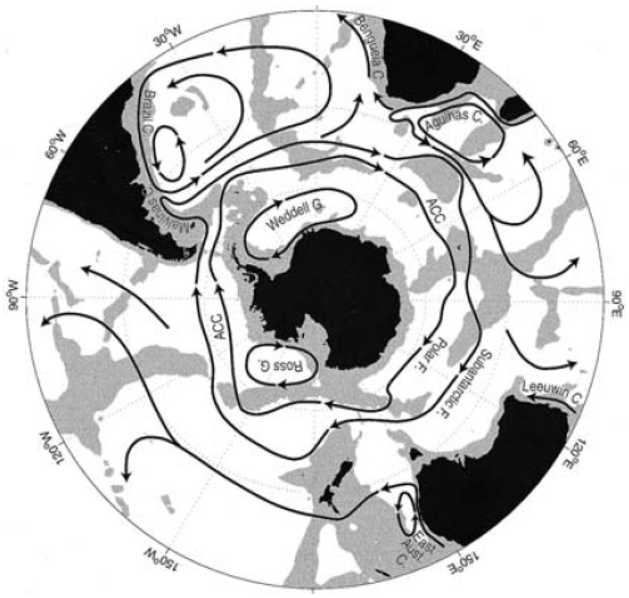
1. Introduction
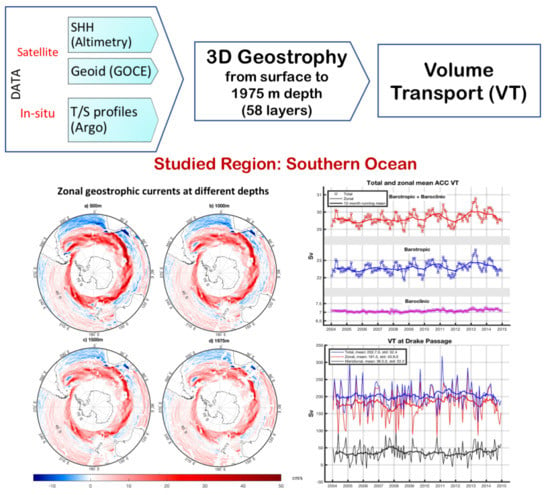
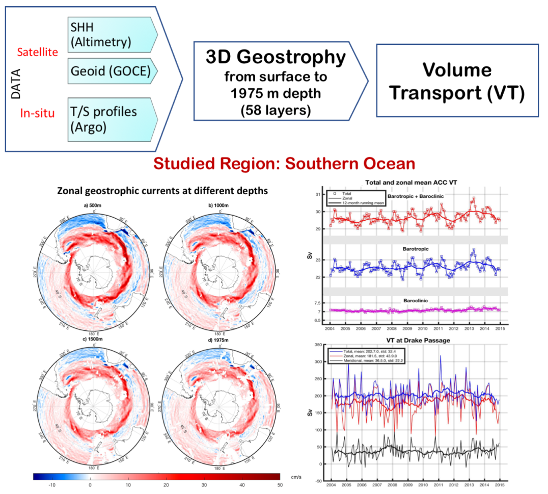
2. Methodology
3. Data
3.1. Sea Surface Height
3.2. Mean Sea Surface, Geoid, and Mean Dynamic Topography
3.3. Temperature and Salinity Profiles from Argo Data
3.4. Simulated Geostrophic Currents from ECCO Model
3.5. In-Situ Observations from Drifters
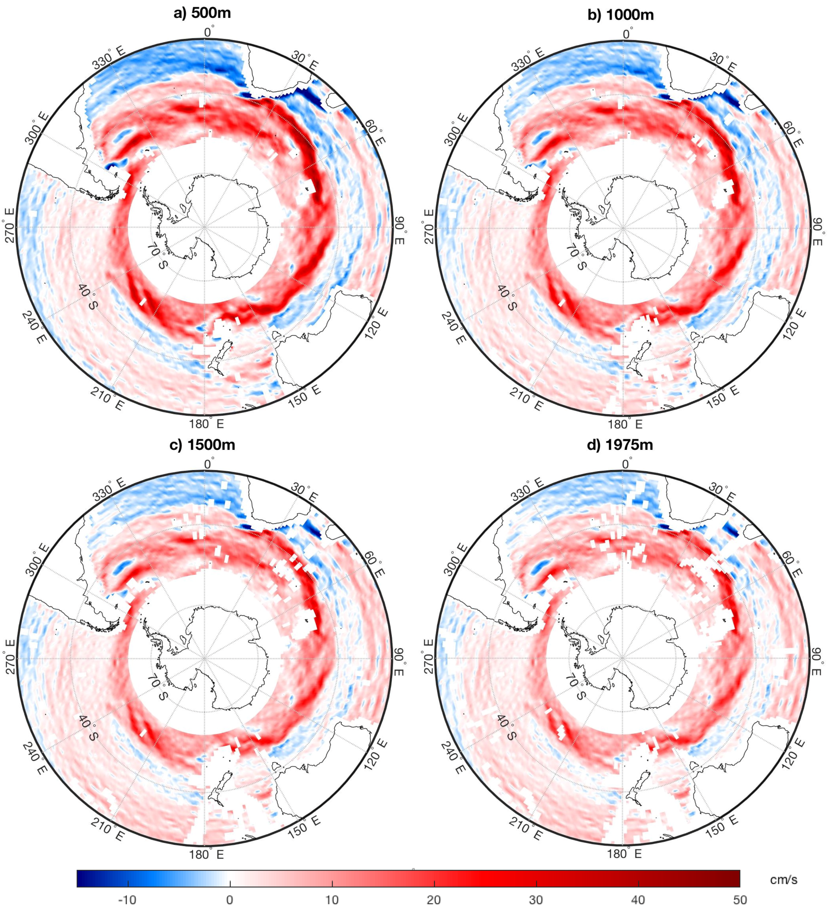
4. Results and Discussion
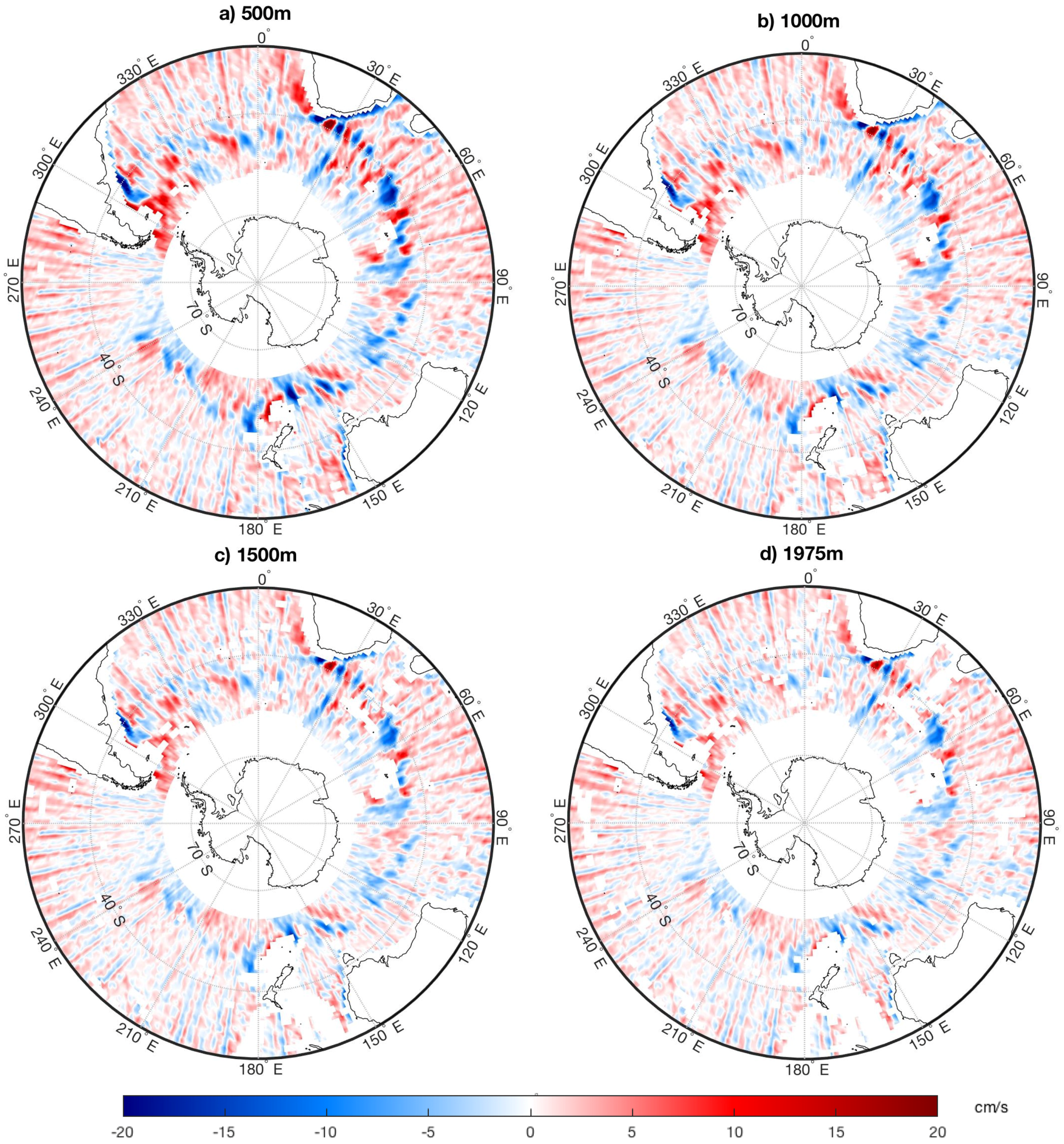
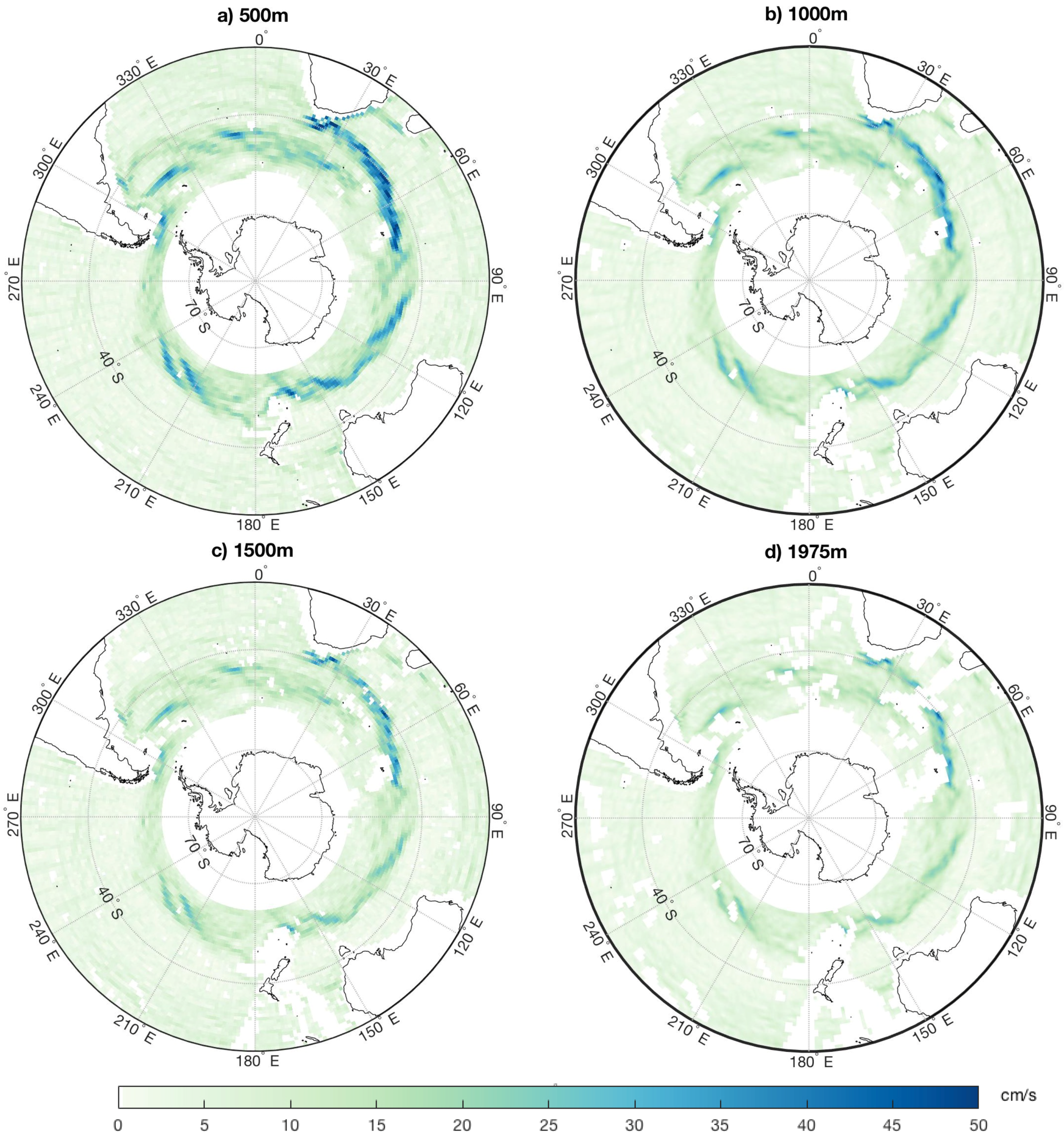
4.1. 3D Geostrophic Currents
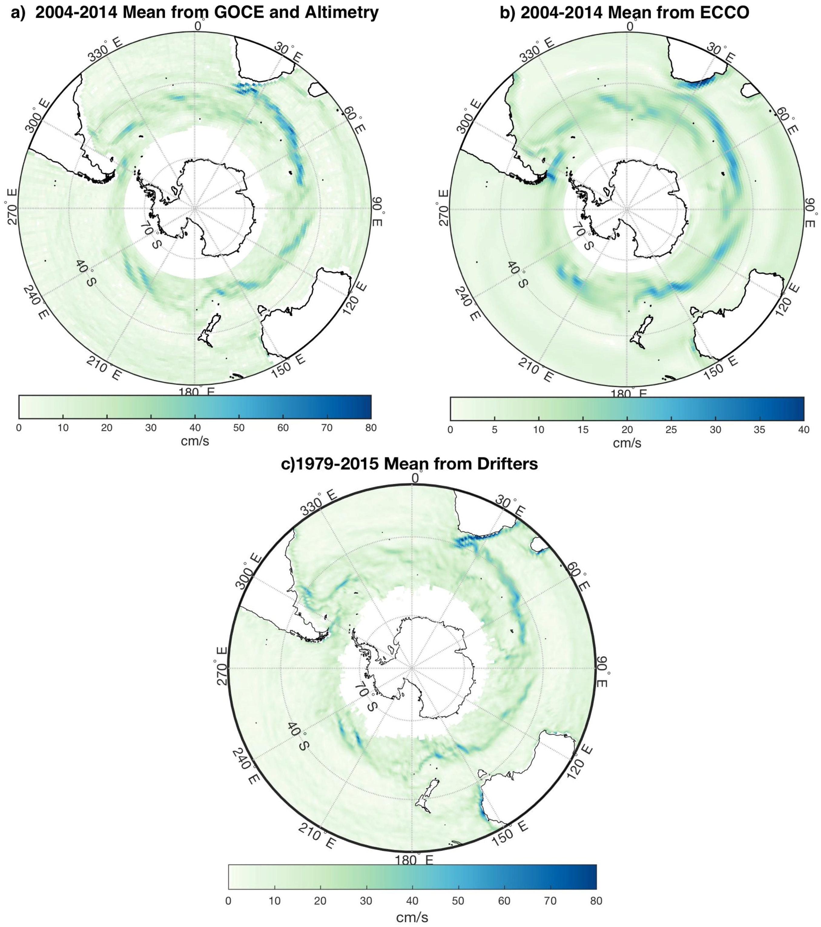
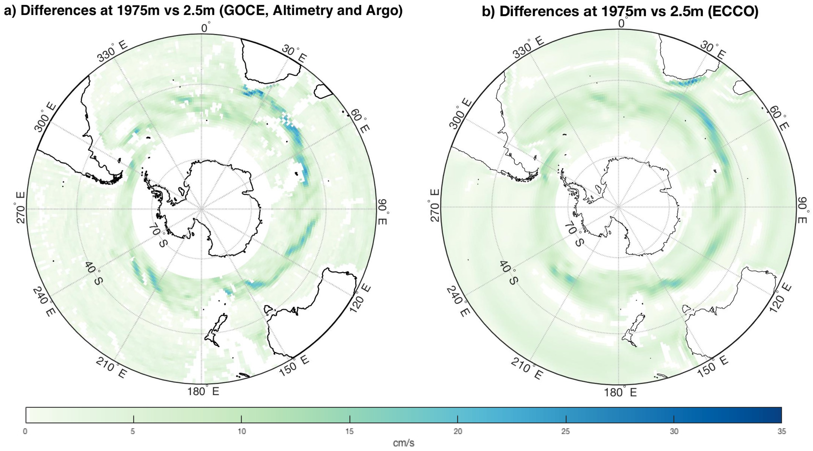
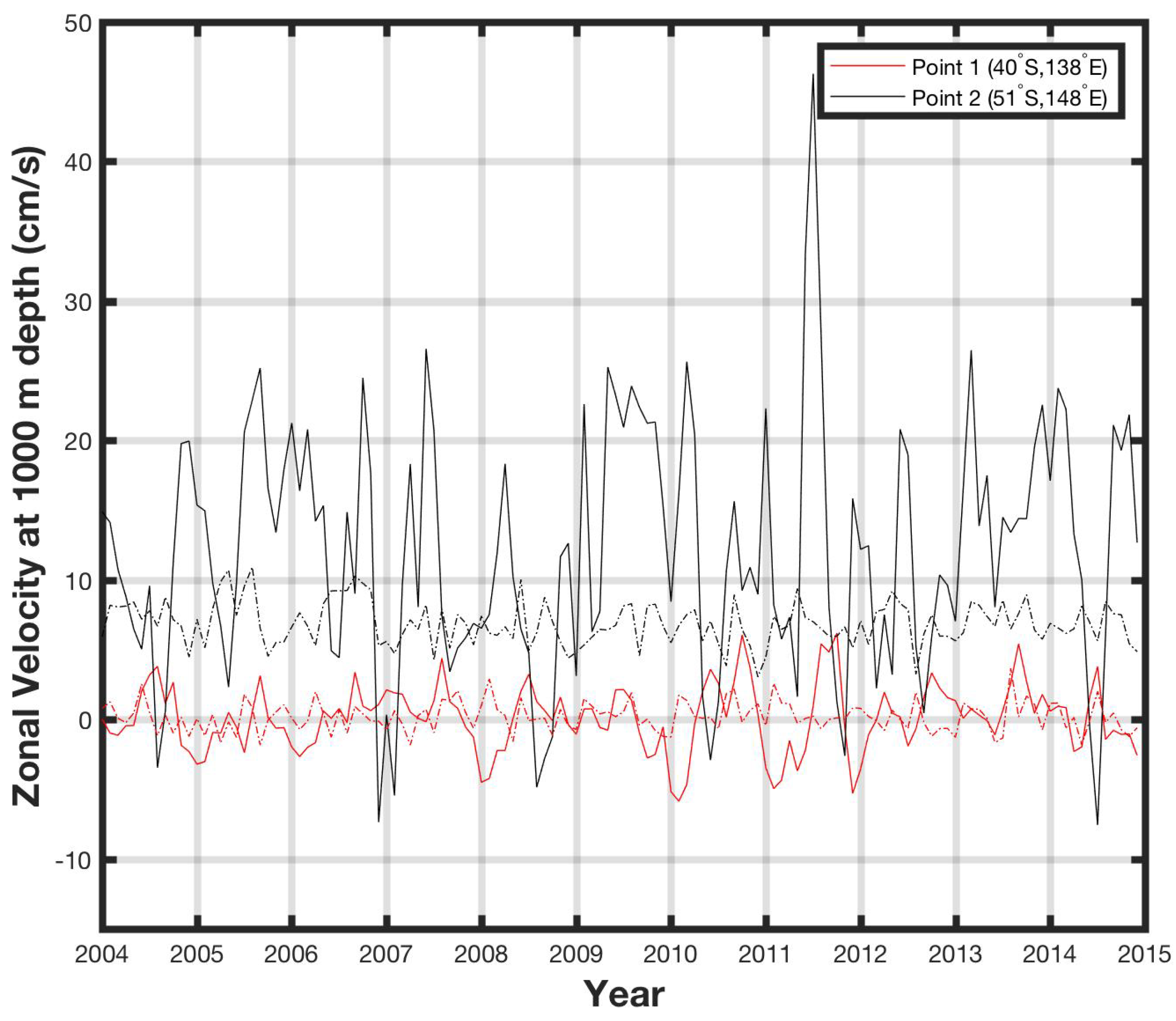
4.2. Comparison with Simulated ECCO geoStrophic Currents and In-Situ Surface Currents Observations
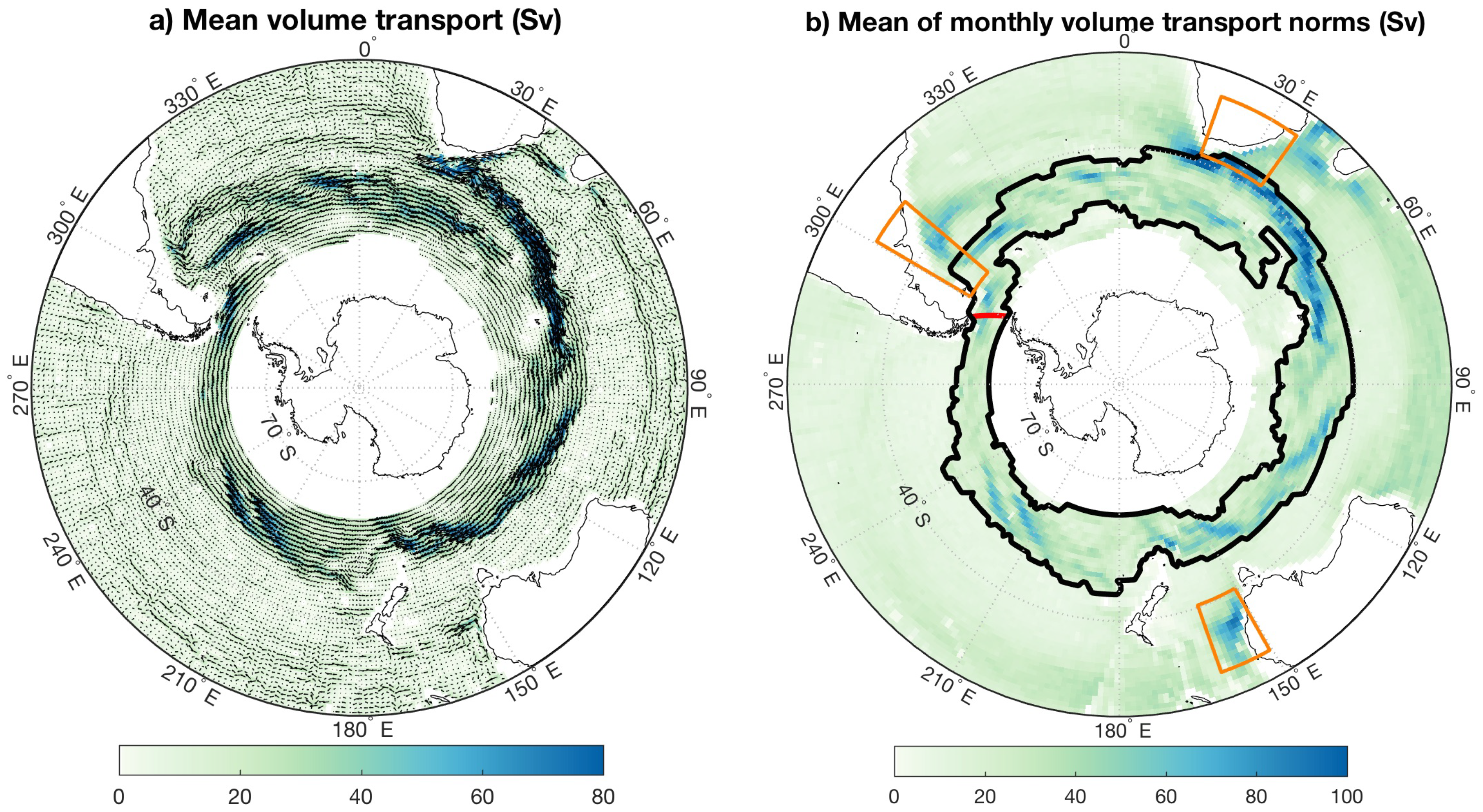
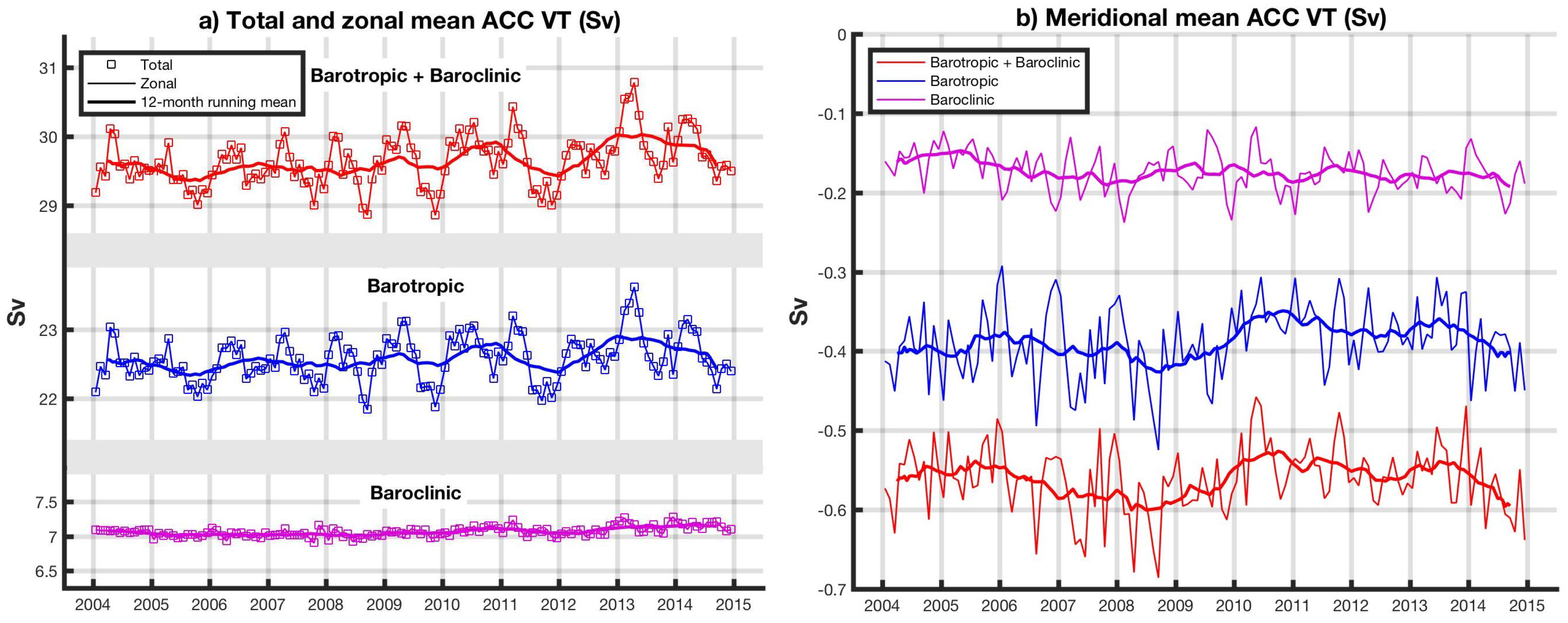
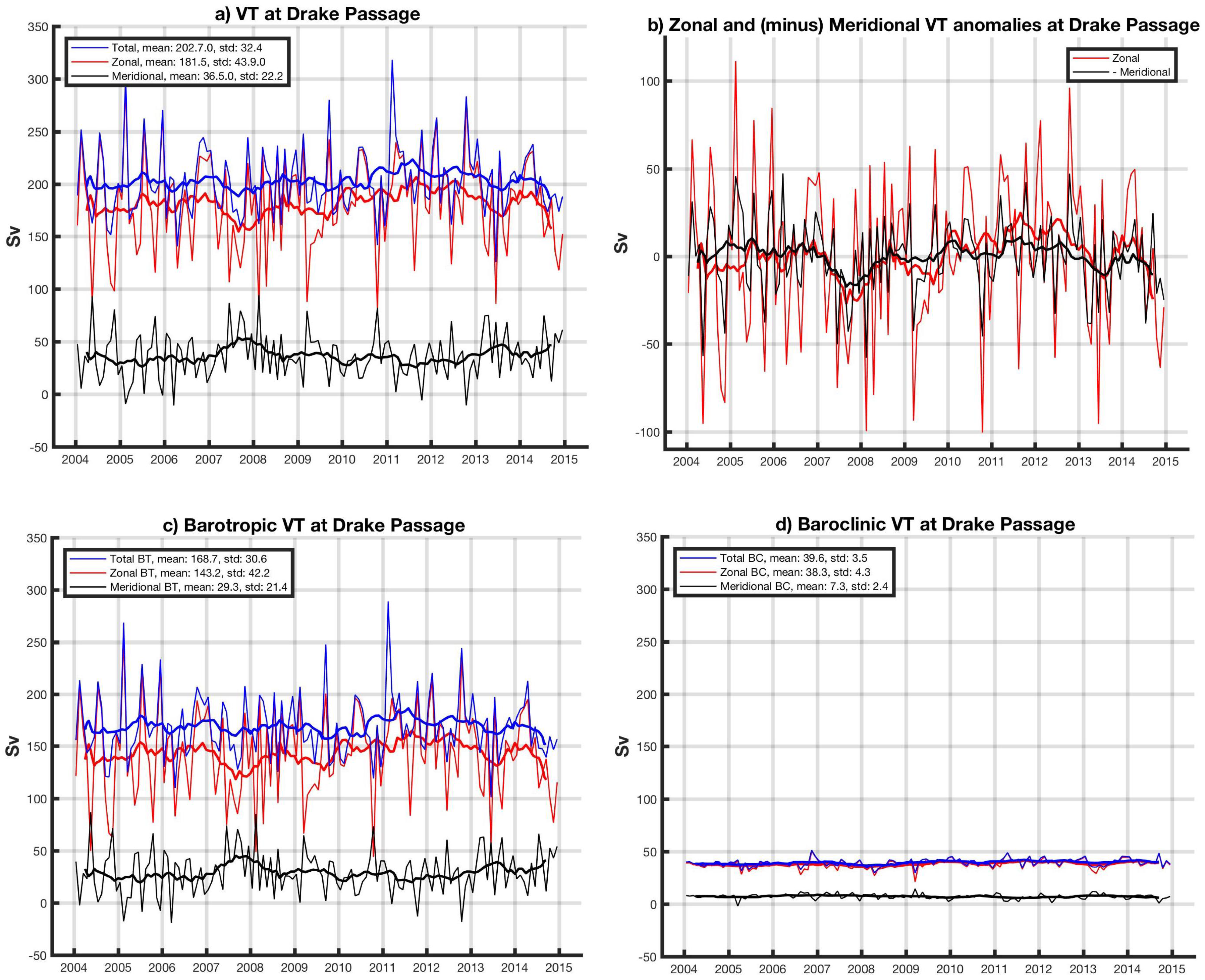
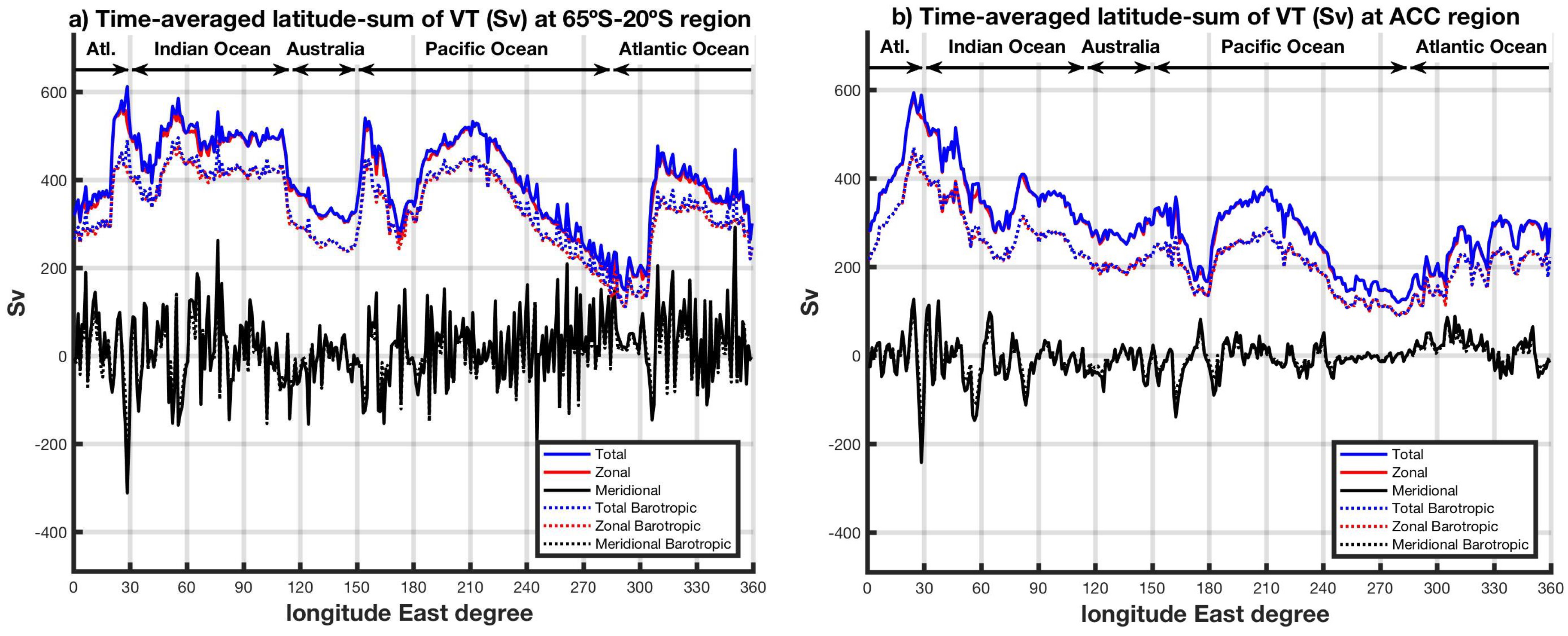
4.3. Volume Transports
5. Conclusions
Author Contributions
Funding
Acknowledgments
Conflicts of Interest
References
- Richardson, P.L. Worldwide ship drift distributions identify missing data. J. Geophys. Res. 1989, 94, 6169–6176. [Google Scholar] [CrossRef]
- Whitworth, T.; Peterson, R.G. Volume Transport of the Antarctic Circumpolar Current from Bottom Pressure Measurements. Am. Meteorol. Soc. 1984, 15, 810–816. [Google Scholar] [CrossRef]
- Donohue, K.A.; Tracey, K.L.; Watts, D.R.; Chidichimo, M.P.; Chereskin, T.K. Mean Antarctic Circumpolar Current transport measured in Drake Passage. Geophys. Res. Lett. 2016, 43, 11760–11767. [Google Scholar] [CrossRef]
- Frankignoul, C.; Bonjean, F.; Reverdin, G. Interannual variability of surface currents in the tropical Pacific during 1987–1993. J. Geophys. Res. 1996, 101, 3629–3647. [Google Scholar] [CrossRef]
- Cunningham, S.A.; Alderson, S.G.; King, B.A.; Brandon, M.A. Transport and variability of the Antarctic Circumpolar Current in Drake Passage. J. Geophys. Res. 2003, 108, 8084. [Google Scholar] [CrossRef]
- Firing, Y.; Chereskin, T.K.; Mazloff, M.R. Vertical structure and transport of the Antarctic Circumpolar Current in Drake Passage from direct velocity measurements. J. Geophys. Res. 2011, 116, C08015. [Google Scholar] [CrossRef]
- Colin de Verdière, A.; Ollitrault, M. A direct determination of the World Ocean barotropic circulation. J. Phys. Oceanogr. 2016, 46, 255–273. [Google Scholar] [CrossRef]
- Wunsch, C.; Gaposchkin, E.M. On using satellite altimetry to determine the general circulation of the oceans with application to geoid improvement. Rev. Geophys. 1980, 18, 725–745. [Google Scholar] [CrossRef]
- Fu, L.L.; Cazenave, A. (Eds.) Satellite Altimetry and Earth Science; Academic Press: New York, NY, USA, 2001; p. 463. [Google Scholar]
- Roemmich, D.; Owens, W.B. The Argo Project: Global ocean observations for the understanding and prediction of climate variability. Oceanography 2000, 13, 45–50. [Google Scholar] [CrossRef]
- Rummel, R.; Balmino, G.; Johannessen, J.; Visser, P.; Woodworth, P. Dedicated gravity field missions—Principles and aims. J. Geodyn. 2002, 33, 3–20. [Google Scholar] [CrossRef]
- Cadden, D.D.H.; Subrahmanyam, B.; Chambers, D.P.; Murty, V.S.N. Surface and subsurface geostrophic current variability in the Indian Ocean from altimetry. Mar. Geod. 2009, 32, 19–29. [Google Scholar] [CrossRef]
- Mulet, S.; Rio, M.H.; Mignot, A.; Guineut, S.; Morrow, R. A new estimate of the global 3D geostrophic ocean circulation based on satellite data and in-situ measurements. Deep Sea Res. II 2012, 77–80, 70–81. [Google Scholar] [CrossRef]
- Kosempa, M.; Chambers, D.P. Southern Ocean Velocity and Geostrophic transport fields estimated combining Jason altimetry and ARGO data. J. Geophys. Res. Oceans 2014, 119, 4761–4776. [Google Scholar] [CrossRef]
- Carter, L.; McCave, I.N.; Williams, M.J.M. Circulation and water masses of the Southern Ocean: A review. Dev. Earth Environ. Sci. 2008, 8, 85–114. [Google Scholar] [CrossRef]
- Rintoul, S.R.; Hughes, C.W.; Olbers, A. The Antarctic Circumpolar Current system. In Ocean Circulation and Climate: Observing and Modelling the Global Ocean; Siedler, G., Church, J., Gould, J., Eds.; International Geophysics 77; Academic Press: New York, NY, USA, 2001; pp. 271–302. ISBN 978-0-12-641351-9. [Google Scholar]
- Rintoul, S.R.; Sokolov, S. Baroclinic transport variability of the Antarctic Circumpolar Current south of Australia (WOCE repeat section SR3). J. Geophys. Res. 2001, 106, 2815–2832. [Google Scholar] [CrossRef]
- Rintoul, S.R.; Sokolov, S.; Church, J. A 6 year record of baroclinic transport variability of the Antarctic Circumpolar Current at 140° E derived from expendable bathythermograph and altimeter measurements. J. Geophys. Res. 2002, 107, 3155. [Google Scholar] [CrossRef]
- Ganachaud, A.; Wunsch, C. Improved estimates of global ocean circulation, heat transport and mixing from hydrographic data. Nature 2000, 408, 453–457. [Google Scholar] [CrossRef] [PubMed]
- Koenig, Z.; Provost, C.; Ferrari, R.; Sennéchael, N.; Rio, M.H. Volume transport of the Antarctic Circumpolar Current: Production and validation of a 20 year long time series obtained from in situ and satellite observations. J. Geophys. Res. Oceans 2014, 119, 5407–5433. [Google Scholar] [CrossRef]
- McDougall, T.J.; Barker, P.M. Getting started with TEOS-10 and the Gibbs Seawater (GSW) Oceanographic 423 Toolbox, version 3.0 (R2010a). SCOR/IAPSO WG 2011, 127, 1–28. [Google Scholar]
- Ablain, M.; Cazenave, A.; Larnicol, G.; Balmaseda, M.; Cipollini, P.; Faugére, Y.; Fernandes, M.J.; Henry, O.; Johannessen, J.A.; Knudsen, P.; et al. Improved sea level record over the satellite altimetry era (1993–2010) from the Climate Change Initiative project. Ocean Sci. 2015, 11, 67–82. [Google Scholar] [CrossRef]
- Andersen, O.; Knudsen, P.; Stenseng, L. The DTU13 MSS (Mean Sea Surface) and MDT (Mean Dynamic Topography) from 20 years of Satellite Altimetry. In IAG Symposia; Springer: Cham, Switzerlands, 2015. [Google Scholar]
- Förste, C.; Bruinsma, S.; Shako, R.; Marty, J.-C.; Flechtner, F.; Abrikosov, O.; Dahle, C.; Lemoine, J.-M.; Neumayer, K.H.; Biancale, R.; et al. EIGEN-6—A new combined global gravity field model including GOCE data from the collaboration of GFZ-Potsdam and GRGS-Toulouse. In Proceedings of the EGU General Assembly, Vienna, Austria, 3–8 April 2011. [Google Scholar]
- Roemmich, D.; Gilson, J. The 2004–2008 mean and annual cycle of temperature, salinity, and steric height in the global ocean from the Argo Program. Prog. Oceanogr. 2009, 82, 81–100. [Google Scholar] [CrossRef]
- Fukumori, I.; Wang, O.; Fenty, I.; Forget, G.; Heimbach, P.; Ponte, R.M. ECCO Version 4 Release 3. 2017. Available online: ftp://ecco.jpl.nasa.gov/Version4/Release3/doc/v4r3_estimation_synopsis.pdf (accessed on April 2018).
- Forget, G.; Campin, J.-M.; Heimbach, P.; Hill, C.N.; Ponte, R.M.; Wunsch, C. ECCO version 4: An integrated framework for non-linear inverse modeling and global ocean state estimation. Geosci. Model Dev. 2015, 8, 3071–3104. [Google Scholar] [CrossRef]
- Sudre, J.; Maes, C.; Garçon, V.C. On the global estimates of geostrophic and Ekman surface currents. Limnol. Oceanogr. Fluids Environ. 2013, 3, 1–20. [Google Scholar] [CrossRef]
- Laurindo, L.; Mariano, A.; Lumpkin, R. An improved near-surface velocity climatology for the global ocean from drifter observations. Deep-Sea Res. I 2017, 124, 73–92. [Google Scholar] [CrossRef]
- Laurindo, L. On the Air-Sea Exchange of Mechanical Energy: A Meso to Large-Scale Assessment Using Concurrent Drifter and Satellite Observations. Ph.D. Dissertation, University of Miami, Coral Gables, FL, USA, 2018. [Google Scholar]
- Zhang, Z.-Z.; Chao, B.F.; Lu, Y.; Hsu, H.-T. An effective filtering for GRACE time-variable gravity: Fan filter. Geophys. Res. Lett. 2009, 36, L17311. [Google Scholar] [CrossRef]
- Johnson, G.C.; Bryden, H.L. On the size of the Antarctic Circumpolar Current. Deep-Sea Res. 1989, 36, 39–53. [Google Scholar] [CrossRef]
- Kundu, P.J. Ekman Veering Observed near the Ocean Bottom. J. Phys. Oceanoghrapy 1975, 6, 238–242. [Google Scholar] [CrossRef]
- Bingham, R.J.; Knudsen, P.; Andersen, O.; Pail, R. An initial estimate of the North Atlantic steady state geostrophic circulation from GOCE. Geophys. Res. Lett. 2011, 38, L01606. [Google Scholar] [CrossRef]
- Feng, G.; Jin, S.; Sanchez-Reales, J.M. Antarctic circumpolar current from satellite gravimetric models ITG-GRACE2010, GOCE-TIM3 and satellite altimetry. J. Geodyn. 2013, 72, 72–80. [Google Scholar] [CrossRef]
- Knudsen, P.; Bingham, R.; Andersen, O.; Rio, M.H. A global mean dynamic topography and ocean circulation estimation using a preliminary GOCE gravity model. J. Geod. 2011, 85. [Google Scholar] [CrossRef]
- Sánchez-Reales, J.M.; Vigo, M.I.; Jin, S.G.; Chao, B.F. Global Surface Geostrophic Currents from Satellite Altimetry and GOCE. In Proceedings of the 4th International GOCE User Workshop, Munich, Germany, 31 March–1 April 2011. ESA SP-696. [Google Scholar]
- Sánchez-Reales, J.M.; Vigo, M.I.; Jin, S.G.; Chao, B.F. Global Surface Geostrophic Currents Derived from Satellite Altimetry and GOCE Geoid. Mar. Geod. 2012, 35, 175–189. [Google Scholar] [CrossRef]
- Fofonoff, N.P. Dynamics of ocean currents. In The Sea. Volume 1: Physical Oceanography; Wiley-Interscience: Hoboken, NJ, USA, 1962; pp. 323–395. [Google Scholar]
- Briden, H.L.; Beal, L.M.; Duncan, L.M. Structure and Transport of the Agulhas Current ant its temporal variability. J. Oceanogr. 2005, 61, 479–492. [Google Scholar] [CrossRef]
- Donohue, K.A.; Firing, E.; Beal, L. Comparison of three velocity sections of the Agulhas Current and Agulhas Undercurrent. J. Geophys. Res. 2000, 105, 28585–28593. [Google Scholar] [CrossRef]
- Sloyan, B.M.; Ridgway, K.R.; Cowley, R. The East Australian Current and Property Transport at 27°S from 2012 to 2013. J. Phys. Oceanogr. 2016, 46. [Google Scholar] [CrossRef]
- Griesel, A.; Mazloff, M.R.; Gille, S.T. Mean dynamic topography in the Southern Ocean: Evaluating Antarctic Circumpolar Current transport. J. Geophys. Res. 2011, 117, C01020. [Google Scholar] [CrossRef]


© 2018 by the authors. Licensee MDPI, Basel, Switzerland. This article is an open access article distributed under the terms and conditions of the Creative Commons Attribution (CC BY) license (http://creativecommons.org/licenses/by/4.0/).
Share and Cite
Vigo, M.I.; García-García, D.; Sempere, M.D.; Chao, B.F. 3D Geostrophy and Volume Transport in the Southern Ocean. Remote Sens. 2018, 10, 715. https://doi.org/10.3390/rs10050715
Vigo MI, García-García D, Sempere MD, Chao BF. 3D Geostrophy and Volume Transport in the Southern Ocean. Remote Sensing. 2018; 10(5):715. https://doi.org/10.3390/rs10050715
Chicago/Turabian StyleVigo, María Isabel, David García-García, María Dolores Sempere, and Ben F. Chao. 2018. "3D Geostrophy and Volume Transport in the Southern Ocean" Remote Sensing 10, no. 5: 715. https://doi.org/10.3390/rs10050715
APA StyleVigo, M. I., García-García, D., Sempere, M. D., & Chao, B. F. (2018). 3D Geostrophy and Volume Transport in the Southern Ocean. Remote Sensing, 10(5), 715. https://doi.org/10.3390/rs10050715