Abstract
Ionosphere research using the Global Navigation Satellite Systems (GNSS) techniques is a hot topic, with their unprecedented high temporal and spatial sampling rate. We introduced a new GNSS Ionosphere Monitoring and Analysis Software (GIMAS) in order to model the global ionosphere vertical total electron content (VTEC) maps and to estimate the GPS and GLObalnaya NAvigatsionnaya Sputnikovaya Sistema (GLONASS) satellite and receiver differential code biases (DCBs). The GIMAS-based Global Ionosphere Map (GIM) products during low (day of year from 202 to 231, in 2008) and high (day of year from 050 to 079, in 2014) solar activity periods were investigated and assessed. The results showed that the biases of the GIMAS-based VTEC maps relative to the International GNSS Service (IGS) Ionosphere Associate Analysis Centers (IAACs) VTEC maps ranged from −3.0 to 1.0 TECU (TEC unit) (1 TECU = 1 × 10¹⁶ electrons/m2). The standard deviations (STDs) ranged from 0.7 to 1.9 TECU in 2008, and from 2.0 to 8.0 TECU in 2014. The STDs at a low latitude were significantly larger than those at middle and high latitudes, as a result of the ionospheric latitudinal gradients. When compared with the Jason-2 VTEC measurements, the GIMAS-based VTEC maps showed a negative systematic bias of about −1.8 TECU in 2008, and a positive systematic bias of about +2.2 TECU in 2014. The STDs were about 2.0 TECU in 2008, and ranged from 2.2 to 8.5 TECU in 2014. Furthermore, the aforementioned characteristics were strongly related to the conditions of the ionosphere variation and the geographic latitude. The GPS and GLONASS satellite and receiver P1-P2 DCBs were compared with the IAACs DCBs. The root mean squares (RMSs) were 0.16–0.20 ns in 2008 and 0.13–0.25 ns in 2014 for the GPS satellites and 0.26–0.31 ns in 2014 for the GLONASS satellites. The RMSs of receiver DCBs were 0.21–0.42 ns in 2008 and 0.33–1.47 ns in 2014 for GPS and 0.67–0.96 ns in 2014 for GLONASS. The monthly stability of the GPS satellite DCBs was about 0.04 ns (0.07 ns) in 2008 (2014) and that for the GLONASS satellite DCBs was about 0.09 ns in 2014. The receiver DCBs were less stable than the satellite DCBs, with a mean value of about 0.16 ns (0.47 ns) in 2008 (2014) for GPS, and 0.48 ns in 2014 for GLONASS. It can be demonstrated that the GIMAS software had a high accuracy and reliability for the global ionosphere monitoring and analysis.
1. Introduction
The ionosphere is part of the Earth’s atmosphere, ranging from 60 to 1000 km above the mean sea level. It is a dispersive medium for the Global Navigation Satellite Systems (GNSS) operating in the microwave band. The GNSS signals traveling through this medium are affected proportionally to the total electron content (TEC), and inversely proportionally to the squared frequency [1]. The GNSS techniques have become an effective type of continuous global scanner of the Earth’s ionosphere, with their unprecedented high temporal and spatial sampling rate [2,3,4,5]. Over the last three decades, our knowledge on the ionosphere conditions has advanced greatly with the effort from a large number of research institutions and scholars [6,7,8,9].
In the context of the International GNSS Service (IGS), several IGS Ionosphere Associated Analysis Centers (IAACs) have developed different techniques in order to provide Global Ionosphere Maps (GIMs) of the vertical TEC (VTEC), since 1998 [5]. The Center for Orbit Determination in Europe (CODE) has been contributing to the IGS ionosphere analysis activities since the establishment of the IGS ionosphere working group in 1998 [10]. The GIMs in IONosphere Map Exchange (IONEX) format [11] are generated using the spherical harmonic (SH) expansion, with Bernese GPS Software (BGS) [12]. The GLObalnaya NAvigatsionnaya Sputnikovaya Sistema (GLONASS) data have been included for the operational ionosphere analysis since 2003.
The Jet Propulsion Laboratory (JPL) was the first institution to measure the ionospheric TEC on global scales, with a worldwide network of 45 dual-frequency GPS receivers in 1993 [13]. The JPL-product IONEX maps are provided with a 15 min temporal resolution and a varying spatial resolution (typically at 5° × 5°), with a Kalman filter-based approach [2]. The JPL/GIM software uses the zeta function in order to select the stations, and it approximates the ionosphere with a modified three-shell model, using a linear composition of bi-cubic splines with 1280 spherical triangles [14].
The European Space Agency/European Space Operations Center (ESA/ESOC) has contributed to the IGS ionosphere working group, since its inception in 1998. The ESA/ESOC still uses a single-layer approach to model the ionosphere through spherical harmonics, with the software IONosphere MONitoring facility ([IONMON] Version 1), and a new 3-dimensional model development is in the coding and testing stage [15].
The Tomographic Ionosphere model software (TOMION) has been developed at the Universitat Politècnica de Catalunya (UPC), since 1995 [16,17]. This software implements a two-layer voxel model with boundary heights of 60–740–1420 km, using only the geometry-free carrier phase measurements [18]. The software has been evolving in different versions in order to be able to process both the ground-based GNSS data and GPS low Earth orbit satellite radio occultation data [19,20].
The Chinese Academy of Sciences (CAS) became a new contributor to the IGS IAACs in 2016 [5]. The approach that is used by CAS for generating the GIM products is the Spherical Harmonic function Plus generalized Trigonometric Series (SHPTS) [21]. The ionospheric VTEC on local and global scales, are individually modeled by the generalized trigonometric series function over each station and the SH expansion with the order and degree of 15.
In 2016, the GNSS Research Center (GRC) of Wuhan University was also recognized as a new member of the IGS IAACs [5]. The global ionosphere model using ground GNSS observations has been developed at the GRC, since 2011 [22]. An inequality-constrained least squares method was proposed, in order to eliminate the non-physical negative values in the VTEC maps [23].
As the demand for ionosphere products has increased in the field of ionospheric physics research and space geodetic applications, it is very important to monitor and analyze the ionosphere reliably and automatically, with high precision. For certain purposes, such as real-time ionospheric applications or a long period reprocess campaign, the computation efficiency of ionosphere modeling should be considered. Thus, a new high-performance global ionosphere mapping software, named the GNSS Ionosphere Monitoring and Analysis Software (GIMAS), which was integrated with the Open Multi-Processing (OpenMP) parallel algorithm [24], was developed at the GRC [25]. In this contribution, we assess the performance of the GIMAS-based GIM products, compared with the legacy IGS IAACs (CODE, JPL, ESA/ESOC, and UPC) and the Jason-2 altimeter data. Considering the significantly different behavior of ionosphere activities in low and high solar activity periods [9], two datasets from 2008 and 2014 are investigated in our experiments. This manuscript is organized as follows. In Section 2, we describe the global ionosphere mapping methodology in detail. In Section 3, we present the data used in our experiments. Section 4 validates the performance of the GIMAS-based GIMs. Section 5 is the discussion and conclusions are drawn in Section 6.
2. Global Ionosphere Mapping Methodology
In general, the code and carrier phase observations for GNSS measurements can be written as follows:
where and are the code and carrier phase measurements from the receiver, , to the satellite, , in frequency, , with the wave length, ; is the geometric distance; is the velocity of light in a vacuum; and are the receiver and satellite clock biases, respectively; is the dispersive ionospheric delay in the code (the delay) and the carrier phase (the advance); is the non-dispersive tropospheric delay; and are the code biases in the receiver and satellite, respectively; is the float carrier phase ambiguity in cycles (including integer ambiguity and uncalibrated phase delays in receiver and satellite); and are multipath in the code and carrier phase, respectively; and and are the observational noises.
From dual-frequency observation equations, the ionospheric delay measurements can be obtained by creating a difference between two given frequencies, as follows:
where is the combined ionospheric delay; and are the differential code biases (DCBs) in the receiver and satellite, respectively. The multipath effect and noise are not included in Equation (2) for clarity.
The precision of the carrier phase was approximately two orders of magnitude higher than that of the code, but it was affected by the unknown ambiguities that introduce a high complexity. A technical method called ‘levelling carrier phase to code’ [13] was proposed in order to remove the ambiguities of the carrier phase and reduce the noise of code. Before the aligning process, the cycle slips were detected and handled, using the method that was proposed by Blewitt [26]. The levelled carrier phase measurements can be expressed as follows:
where is the average in a continuous arc.
The ionospheric delay could be expressed up to the third order, and the first order term (with a dependence on ) accounted for more than 99.9% of the total ionospheric delay. The higher-order ionospheric delay may exceed 10 mm (0.1 TECU [TEC Unit], 1 TECU = 1 × 10¹⁶ electrons/m2) [27], but the magnitude was very small in the global ionosphere mapping. The ionospheric delay could be expressed with a good approximation, without the higher-order ionospheric delay, as follows:
where is the Slant TEC (STEC) from the receiver, , to the satellite, .
The SH expansion model was widely used to represent the global and regional VTEC in the spatial and temporal domains [28]. An infinitely thin shell at an altitude of 450 km above the Earth was assumed, where the TEC was concentrated for simplicity. The ionosphere pierce points (IPPs) were the points where the signal path and the thin shell intersect. The STEC along the signal path was mapped to VTEC through a modified mapping function [12]. The SH expansion model and modified mapping function could be expressed as follows:
where is the vertical TEC; and are the latitude and longitude of IPPs in solar-geomagnetic reference frame; is the normalized associated Legendre function with the degree, , and order, , and was set at 15 in our research; and are the SH expansion coefficients; is the satellite zenith at the station; (~6371 km) is the radius of the Earth; (~506.7 km) is the altitude for modified mapping function only and it should be noted that the altitude here is different from the altitude (450 km) for the thin shell [12]; and is a correction factor that was set at 0.9782.
According to Equations (3)–(5), the global ionospheric model can be derived from the GNSS code and carrier phase observations as follows:
where the SH expansion coefficients and DCBs in the satellite and receiver are unknown parameters and are estimated simultaneously.
Since the satellite and receiver DCBs are strongly correlated, the normal equation matrix is rank deficient. A zero-mean constraint [12] on the satellite DCBs was applied for each satellite system, as follows:
where is the total number of operational satellites for each satellite system; indicates the satellite system.
Since the ionospheric electron distribution that was produced by the ionization was driven by the solar radiation and ordered by the geomagnetic field of the Earth [29], the SH expansion was expressed in solar-geomagnetic reference frame [2]. In this reference frame, theoretically speaking, one set of SH expansion coefficients could be estimated to express the VTEC map daily, as early ionosphere products at CODE [10]. In practice, sets of coefficients are estimated so as to characterize the sub-daily variation. In our research, the interval between the sessions was set at two hours. Considering the continuity of the SH expansion coefficients between consecutive days, 28 h (one day and two hours before the day and two hours after the day) observations were used to estimate 15 sets of coefficients. A Piecewise Linear (PWL) interpolation strategy [12] was applied between the consecutive sets of coefficients as follows:
where is the coefficient at arbitrary time, , between session and ; and are the coefficients at the session times and .
Most of the stations were distributed in the Northern Hemisphere, especially in the European and American continents. However, within a solar-geomagnetic reference frame, the SH expansion coefficients represented the global VTEC for a given time and not for a given geographical station distribution [30]. Whether or not a region was populated with GNSS receivers, it would sample a full range of times for one day. Therefore, the VTEC values in the regions that were lacking receivers at a given local time were estimated or predicted by measurements that were obtained, at that same local time, from receivers in the same geomagnetic latitude band [30]. The VTEC that was estimated in those regions were extrapolated in time, so the precision was significantly lower than that in the regions with actual measurements. A compromise should have been made between the measurement coverage and the time resolution. In the sun-fixed reference frame, the global VTEC was almost frozen in a short time and the SH expansion coefficients varied slowly. Based on this fact, the random walk could be used to represent the variation of the SH expansion coefficients with time. The SH expansion coefficients at different sessions, using random walk, could be expressed as follows:
where the empirical mean value of the random walk was assumed to be 0.
The weight of the random walk constraint was determined according to its power spectral density, and it was very important to balance the weight between the observations and the random walk constraint. The power spectral density was set at 2.0–5.0 TECU/hour1/2 with experience, according to the ionospheric variations [2]. As a result of the uneven station distribution, the estimated VTEC maps, using the SH expansion model, would have had negative values (replaced with zero in ESA- and CODE-product IONEX maps) at high latitude regions, especially in the low solar activity years. To overcome this drawback, the inequality-constrained least squares method [23] was used in our study.
For the mapping of the daily global ionosphere, millions of observations were used. It was very effective to manipulate and stack a normal equation matrix in a mathematical way, for each individual normal equation system [25]. All of the strategies or constraints were added to the normal equation matrix in the same way. The form of the normal matrix is similar to Figure 1 in Zhang et al. [23]. The parameters, including the SH expansion coefficients and DCBs in the satellite and receiver, were estimated by the constrained least squares adjustment. The solutions and estimated standard deviations were computed as follows:
where and are the normal equation matrix for observations and right hand side of the normal equations, respectively; is the design matrix; is the weight matrix of the observations; is the array of the actual observations; the matrix for the DCB constraint, piecewise linear interpolation strategy, random walk constraint, and inequality constraint is similar to that for observations; and is the posteriori standard deviation of unit weight.
The global ionosphere mapping methodology that was used in our experiments is summarized in Table 1. The differences between the IAACs (CODE, ESA/ESOC, JPL, and UPC) are also compared.

Table 1.
Summary of different techniques and implementations at the Ionosphere Associated Analysis Centers (IAACs).
3. Data Processing
The ionosphere variation was correlated with the solar activity and the geomagnetic activity [31]. Figure 1 shows the mean global TEC (MGEC) [12] evolution from 1998 to 2016, and it is equivalent to the Global Electron Content (GEC) that was proposed as the ionospheric index in the work of Afraimovich, E.L. et al. [32]. The global signature of the solar cycle as well as the annual and seasonal periods were evident. The evolution of MGEC coincided with that of the solar flux remarkably well. To validate the performance of the GIMAS-based GIMs, two datasets were performed during low (day of year [Doy] from 202 to 231, 2008) and high (Doy from 050 to 079, 2014) solar activity years. In the low solar activity period, the MGEC ranged from 6 to 9 TECU, while it ranged from 32 to 45 TECU in the high solar activity period.
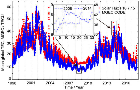
Figure 1.
The mean global total electron content (TEC) evolution (blue) derived from the Center for Orbit Determination in Europe (CODE) Global Ionosphere Maps (GIMs) versus the solar flux F10.7 index (red) from 1998 to 2016. Two datasets were selected indicating the low (2008) and high (2014) solar activity periods. MGEC—mean global TEC; TECU—TEC unit.
In our research, about 300 IGS stations [33] were selected to generate the daily GIM, and the stations distribution is shown in Figure 2. Most of the stations were installed in the Northern Hemisphere continents, and only a few of the stations were located on islands in the oceanic areas. It was expected that the precision of the VTEC map over the continents would be much higher than that over the oceans.
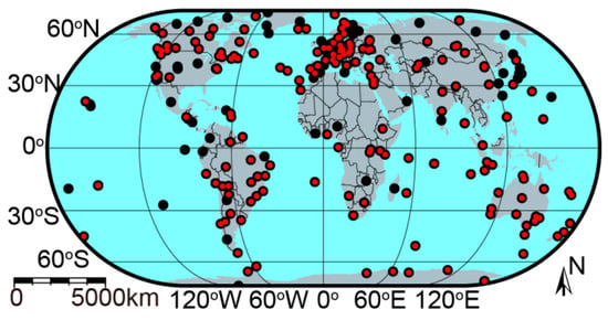
Figure 2.
Distribution of International GNSS (Global Navigation Satellite Systems) Service (IGS) tracking stations with GPS (black) or GPS/GLObalnaya NAvigatsionnaya Sputnikovaya Sistema (GLONASS) (red) data on the day of year (Doy) 050, 2014. The numbers of stations with GPS or GPS/GLONASS data are 299 and 195, respectively.
The experiments were supported with the GIMAS software, which was developed at the GRC of Wuhan University [25]. The core modules of the software were programmed by C++ language, and the automatic scripts were written by the Shell language that was working under the Linux system. To improve the computation efficiency, a parallel computing technique, called OpenMP, was incorporated into the software [25]. The software has currently been used for the daily ionosphere monitoring and analysis at the GRC. The flowchart of the software is shown in Figure 3. The yellow rectangles represent the parallel computing stages. The time for the daily GIM generation was only about 10–13 min, with 24 processors [25].
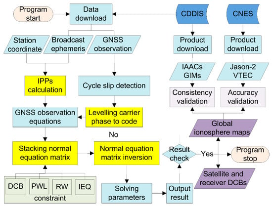
Figure 3.
The GNSS Ionosphere Monitoring and Analysis Software (GIMAS) software flowchart. CDDIS—Crustal Dynamics Data Information Center; CNES—Centre National d’Etudes Spatiales; VTEC—vertical total electron content; IPPs—ionosphere pierce points; DCB—differential code biases; PWL—Piecewise Linear; RW—Random Walk; IEQ—Inequality constraint.
4. GIMAS-Based GIMs Performance Validation
The daily GIM contained a 13 VTEC and root mean square (RMS) maps with a 2 h resolution. The latitude ranged from 87.5°N to 87.5°S, with a 2.5° resolution, and the longitude ranged from 180°W to 180°E, with a 5.0° resolution. Along with the VTEC maps, the GPS and GLONASS satellite and receiver DCBs were produced simultaneously. Firstly, the differences between the GIMAS-based VTEC maps and the IAACs VTEC maps were discussed. Then, the accuracy of GIMAS-based VTEC maps was analyzed in comparison to the Jason-2 VTEC measurements. Finally, the DCBs in the satellites and receivers were compared with the IAACs DCB products. The VTEC maps or DCBs from the four IAACs were denoted as CODE, JPL, ESA, and UPC, respectively, and the estimates that were derived from the GIMAS software were denoted as GRC.
4.1. VTEC Validation Compared with IAACs VTEC Maps
Although the VTEC maps were generated at different IAACs, with different techniques or implementations, the global VTEC maps could be represented with the standard IONEX format, which used 5183 grid points to describe the ionosphere at each session. As a result, it was very convenient to compare the products that were derived from different centers, and a combined IGS GIM product, named IGSG, could be generated by considering all of the advantages, as shown in Hernández-Pajares et al. [4]. In this section, the differences of VTEC maps, between the GRC and IAACs, were calculated with the bias and standard deviation (STD) indices in Equation (11).
where and are the VTEC derived from the GRC and IAACs, respectively; and denotes the average calculating operation.
Figure 4 shows the global VTEC snapshots that were determined by the GRC and IAACs for Doy 202, 2008 and Doy 050, 2014, taken at 06:00 Universal Time (UT). The models had expressed the global VTEC distribution well, both in longitude and latitude. The maximum VTEC was located around the longitude 90°E at 06:00 UT (the Earth rotates 15 degrees in one hour). The well-known ionospheric equatorial anomaly (a double-humped structure with a trough centered around the geomagnetic equator and two crests on either side of it, around 18° geomagnetic latitude) was very clear in the maps. On Doy 202, 2008, the maximum VTEC was only about 24 TECU, while it was about 120 TECU on Doy 050, 2014. Although the global ionosphere modeling methods were different, the VTEC differences between the GRC and IAACs were very small during both the low and high solar activity periods.
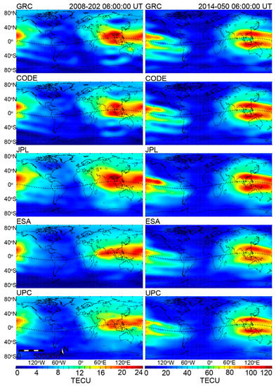
Figure 4.
VTEC maps at 06:00 UT, determined by the GRC and Ionosphere Associated Analysis Centers (IAACs) for Doy 202, 2008 (left panel) and Doy 050, 2014 (right panel). The legend for 2008 is from 0 to 24 TECU, and that for 2014 is from 0 to 120 TECU. The dotted line is the geomagnetic equator. GRC—GNSS Research Center; CODE—Center for Orbit Determination in Europe; JPL—Jet Propulsion Laboratory; ESA—European Space Agency; UPC—Universitat Politècnica de Catalunya.
Figure 5 shows the daily bias and STD of the GRC VTEC maps, relative to the IAACs. It was seen that the bias between the GRC and IAACs varied from −3.0 to 1.0 TECU. The biases of the GRC that was relative to the IAACs in 2008 showed less variability than that in 2014, as a result of the smaller ionospheric variations. The biases of the GRC relative to CODE and JPL did not change much from 2008 to 2014, while those that were relative to ESA and UPC showed considerable variations. In the low solar activity year, the STDs ranged from 0.7 to 1.9 TECU, however they changed from 2.0 to 8.0 TECU in the high solar activity year. Although the STDs in 2014 were significantly larger than those in 2008, the values were still within the accuracy range of 2–8 TECU for the IGS GIM products [4]. The evolution of the STD in 2014 agreed well with that of the MGEC in Figure 1. A rapid drop on Doy 059, 2014 was very evident in both the STD and MGEC. The difference between the GRC and CODE was the least with a mean bias less than 1.0 TECU, and the STD was about 0.7 and 2.0 TECU in 2008 and 2014, respectively.
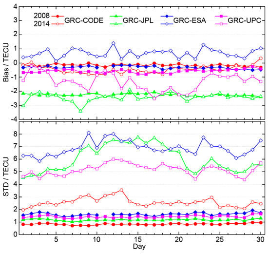
Figure 5.
GRC VTEC maps daily bias (top plot) and standard deviation (STD) (bottom plot), relative to the IAACs for Doy 202–231 in 2008 and Doy 050–079, in 2014.
Considering the ionospheric VTEC latitudinal gradients, the VTEC differences were divided into six geomagnetic latitude bands. The six bands were as follows: the northern high latitude (NHL) (from 87.5°N to 60°N), northern middle latitude (NML) (from 60°N to 30°N), northern low latitude (NLL) (from 30°N to 0°), southern high latitude (SHL) (from 87.5°S to 60°S), southern middle latitude (SML) (from 60°S to 30°S), and southern low latitude (SLL) (from 30°S to 0°). The bias and STD of GRC VTEC maps relative to the IAACs at different geomagnetic latitude bands are shown in Figure 6. The biases at different bands ranged from −4.0 to 2.0 TECU. The bias between the GRC and CODE showed the minimum discrepancies both in 2008 and 2014, mainly because of the same ionospheric models. Although the SH expansion was also used at the ESA, the positive biases were very clear between the GRC and ESA at the low latitude during the high solar activity period (2014). One possible reason was that the VTEC crests at the low latitude were decreased because of the influence of the previous normal equations, when the Kalman filter was used [15]. The VTEC estimates at SHL from the GRC were about 0.7 TECU larger than those from the CODE and ESA in 2008, because of the inequality-constrained least squares. The VTEC estimates from the GRC were 2–3 TECU smaller than those from the JPL. This was because the method that was used at the JPL considered the ionospheric local variation and the data gaps were interpolated with splines [2]. While the SH expansion considered the global variation, the VTEC that was estimated over the oceans might have been underestimated, especially in the Southern Hemisphere. Compared with the UPC, the biases were apparently negative the middle and high latitudes. Apart from the reason of the VTEC interpolation method, another important reason was the two-layer tomographic model [18] at the UPC against the one-layer SH expansion model at the GRC. The STDs ranged from 0.5 to 1.8 TECU in 2008 and from 0.9 to 8.6 TECU in 2014. The STDs at the low latitude were significantly larger than those at the middle and high latitudes, because of the strong ionosphere variation at the low latitude. The STDs in the Northern Hemisphere were smaller than those in the Southern Hemisphere, which might have been related to the denser distribution of stations. The STD differences between the IAACs were small in 2008, but they were very large in 2014, especially at the low latitude. This implied that it was more difficult to model the ionosphere during the high solar activity period. The STDs of the GRC–JPL and GRC–UPC were very large when compared with those of the GRC–CODE, because of the different ionosphere models that were used. However, the STDs of the GRC–ESA were at the maximum and were very different from those of the GRC–CODE, although the same SH expansions were used at the GRC, CODE, and ESA. This indicated that the strategies or constraints in the global ionosphere mapping should be carefully handled.
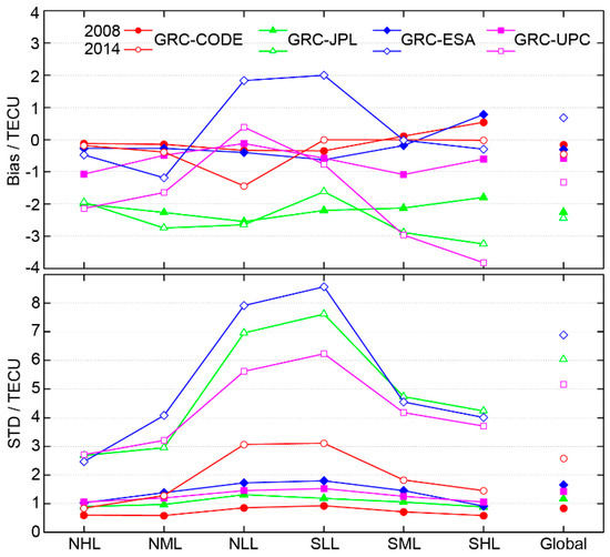
Figure 6.
The GRC VTEC map bias (top plot) and STD (bottom plot) relative to the IAACs at different geomagnetic latitude bands.
4.2. VTEC Validation Compared with Jason-2 Altimeter Data
The radar altimetry derived VTEC was a GNSS-independent data source that was used to validate the accuracy of the GNSS derived VTEC [5], despite the systematic bias to the order of a few TECU [34]. The satellite altimetry missions, such as the TOPEX/POSEIDON, and its follow-on missions Jason-1, Jason-2, and Jason-3, provided the VTEC measurements using the C-band (5.3 GHz) and Ku-band (13.6 GHz) observations since 1992 [35]. These radar altimetry observations were direct vertical measurements that were taken over the oceans with an altitude of 1336 km and an orbit inclination of 66.15°. It should be noted that the vertical measurements of the Jason-2 satellite did not contain the plasmaspheric electron content (PEC), which ranged from 1336 km (Jason-2 orbit altitude) to 20,200 km (GPS orbit altitude) [36].
Figure 7 shows the distribution of ionospheric IPPs of the Jason-2 satellite and the VTEC comparison between the GRC and Jason-2 on Doy 050 in 2014. It can be seen that the IPPs of the Jason-2 satellite ranged approximately from 66°N to 66°S, and only covered the oceans. The GRC VTEC was derived according to the time and footprint location of the Jason-2 satellite, which meant that the GRC VTEC was actually spatially extrapolated far away from the observing stations. There were about 26 passes across one day, and the VTEC gradients along the latitude could be well captured. The bottom left plot shows the full one-to-one comparison between the GRC and Jason-2 from one day. The result showed an overall agreement and a small TECU bias could be observed, which is also shown in Figure 8. For a clear comparison, an example of the GRC VTEC versus Jason-2 VTEC is shown in the bottom right plot. It should be noted that the Jason-2 VTEC was sampled at almost every second and was smoothed with a sliding window of 18 s, in order to reduce the noise [37].
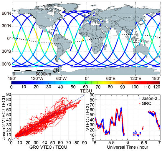
Figure 7.
Distribution of the ionospheric IPPs (top panel) of the Jason-2 satellite and VTEC comparison (bottom panel) between the GRC and Jason-2 on Doy 050 in 2014.
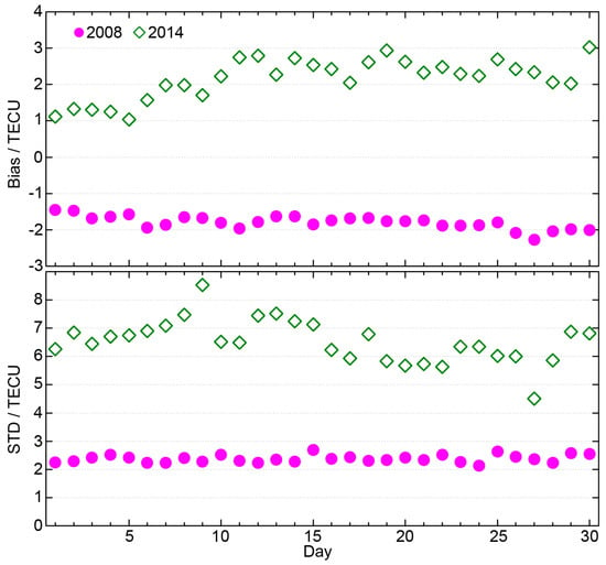
Figure 8.
The GRC VTEC daily bias (top plot) and STD (bottom plot), relative to the Jason-2 VTEC for Doy 202–231 in 2008 and Doy 050–079 in 2014.
The bias and STD indices of the VTEC differences between the GRC and Jason-2 were calculated for comparison. In this section, the VTEC differences denoted the GRC VTEC, minus the Jason-2 VTEC, which was emphasized here for a better understanding of the negative or positive bias that is discussed below. The daily bias and STD of the GRC VTEC, relative to the Jason-2 VTEC of the two datasets in 2008 and 2014, are presented in Figure 8. In the high solar activity year (2014), a positive bias of about +2.2 TECU was observed, while a negative bias of about −1.8 TECU was observed in the low solar activity year. An unexpected negative bias was also observed for the IAACs in both the Northern and Southern Hemisphere from 2003 to 2008 [21], where the negative differences were stronger in the Southern Hemisphere, especially in the southern winter [38]. The positive bias makes sense, given the existence of the PEC, but it was only observed in the high solar activity year (2014), as well as during 2001 and 2002 [36]. This suggested that either the VTEC that was derived from the GNSS was underestimated, or that the Jason-2 VTEC was overestimated during the low solar activity years. The STD was about 2.3 and 6.6 TECU in 2008 and 2014, respectively. The pattern of the GRC-Jason-2 STD also followed that of the MGEC, in Figure 1, where it rose on Doy 058 and dropped on Doy 076, in 2014.
Figure 9 shows the bias and STD of the GRC VTEC, relative to the Jason-2 VTEC at different geomagnetic latitude regions. In 2008, the biases ranged from −4.7 to 0.0 TECU, and the negative bias in the Southern Hemisphere was stronger than that in the Northern Hemisphere. In 2014, the bias at the low and middle latitudes was generally positive, and the value and shape, in terms of the latitude, were similar to the PEC value that was obtained from the TOPEX GPS dual-frequency observations in March 1993 [39]. The ionospheric equatorial anomaly was evident in both 2008 and 2014, where a trough in 2014 was around the equator, while it was around 18°N in the Northern Hemisphere in 2008. The STD in 2008 was about 2.0 TECU, while it ranged from 2.2 to 8.5 TECU, with respect to the latitude, in 2014. The STD at the low latitude was significantly larger than that at the middle latitude, and the value in the Northern Hemisphere was smaller than that in the Southern Hemisphere. The reason for this might have been the mismodeling of the ionospheric VTEC at low latitude, and the sparse distribution of the IGS stations in the Southern Hemisphere. At high latitude regions that were above 60 degrees in the Southern Hemisphere, an apparent bias was observed, especially in 2008. The most possible reason was the mismodeling of ionospheric VTEC at the high latitude in the low solar activity year, although the inequality-constrained least squares method was used to eliminate the negative values [23].
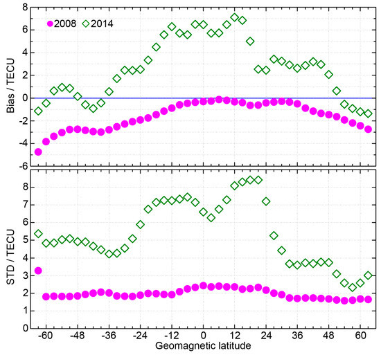
Figure 9.
The GRC VTEC bias (top plot) and STD (bottom plot), relative to the Jason-2 VTEC at different geomagnetic latitudes.
4.3. GPS and GLONASS Satellite DCBs Validation with IAACs DCBs
The inter-frequency satellite DCBs between the P1 and P2 code were estimated in our research. It was known that the satellite DCBs were very stable in a short period and could be considered as constant for one day [40]. The GPS and GLONASS satellites’ DCBs were compared with the IAAC DCBs in this section.
The monthly GPS satellite P1-P2 DCBs for Doy 050–079 in 2014, are presented in Figure 10. The individual satellites were labeled by their pseudo-random noise (PRN) number and were classified under five different blocks. It could be seen that the GPS satellite DCBs mainly varied between −9.0 and 8.0 ns, and that the estimates of the GRC and IAACs were very similar. The same block satellites showed nearly the same amount, which indicated that the characteristics of the DCBs were mainly related to the performance of the corresponding instruments.
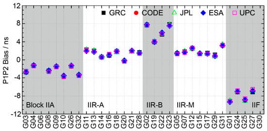
Figure 10.
GPS satellite P1-P2 DCB estimates of the GRC and IAACs for Doy 050–079 in 2014. The GPS satellites were classified under five blocks, namely, Block IIA, Block IIR-A, Block IIR-B, Block IIR-M, and Block IIF.
Figure 11 presents the monthly GLONASS for satellite P1-P2 DCBs for Doy 050–079 in 2014. Only the CODE and ESA had used both the GPS and GLONASS data in order to establish their global ionosphere models during this period. The GLONASS satellites were sorted by the frequency channel number. It is shown that the GLONASS satellite DCBs mainly varied between −9.0 and 6.0 ns. Unlike the GPS DCB estimates, the GLONASS estimates had a notable dependency on the frequency channel number, which might have been attributed to the inter-channel biases for GLONASS with the frequency division multiple access (FDMA) technique [41]. The estimates from the GRC, CODE, and ESA agreed well for most satellites, but the R10(−7), R13(−2), R16(−1), and R15(0) exhibited apparent discrepancies. These discrepancies might have been caused by the different types of receivers that had an impact on the satellite DCBs estimation [42].
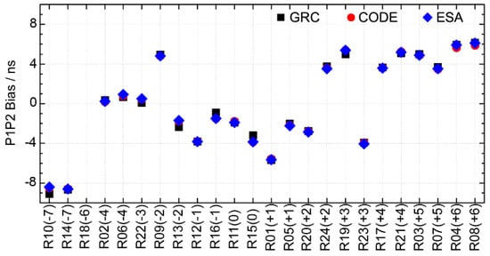
Figure 11.
The GLONASS satellite P1-P2 DCB estimates of the GRC, CODE, and ESA for Doy 050–079 in 2014. The GLONASS satellites were identified by the slot number followed by the frequency channel number in brackets.
Figure 12 shows the mean bias and STD of the GPS satellite P1-P2 DCB estimates for Doy 202–231 in 2008 and Doy 050–079 in 2014. The bias between the different IAACs in 2014 was larger than that in 2008. This might have been caused by the greater differences in the VTEC maps from the IAACs in 2014, which were estimated simultaneously with the DCBs. The DCBs at the UPC showed great discrepancies when compared with the others in both 2008 and 2014, because of the different DCBs estimation method [18]. The bias between the different satellites from the GRC that were relative to the IAACs, had a mean bias of about −0.4 to 0.5 ns in 2008, while the bias varied between −0.3 and 0.3 ns in 2014. The systematical change of the satellite DCB estimates might have been affected by the different tracking network and employed receivers [43]. The STD of the DCB differences was about 0.02–0.15 ns in 2008 and 0.05–0.24 ns in 2014. The STD increased significantly because of the higher variability of the ionosphere in the high solar activity year. The difference between the GRC and CODE was the least, because of the similar estimation method in both 2008 and 2014. The RMS of the DCB differences was about 0.03–0.46 ns in 2008 and 0.05–0.34 ns in 2014. The mean STDs and RMSs are presented in Table 2. The mean RMS for the GRC–ESA differences had a minimum of about 0.16 ns in 2008, however the minimum was only 0.13 ns between the GRC and CODE in 2014, because of a decrease in the bias.
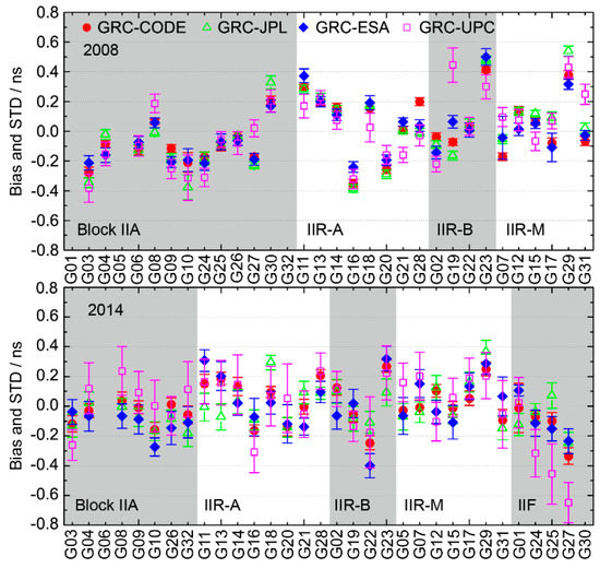
Figure 12.
The bias and STD of the GRC GPS satellite P1-P2 DCB estimates, relative to the IAACs for Doy 202–231 in 2008 (top plot) and Doy 050–079 in 2014 (bottom plot). The dots denote the mean of the differences of the corresponding satellite, and the length of the vertical lines denote the respective standard deviations.
Table 2.
The standard deviation (STD) (before the comma) and root mean square (RMS) (after the comma) of the GRC satellite P1-P2 DCB estimates, relative to the IAACs for Doy 202–231 in 2008 and Doy 050–079 in 2014 (unit: ns).
The mean bias and STD of the GLONASS satellite P1-P2 DCB estimates for Doy 050–079 in 2014, are shown in Figure 13. The difference in the GRC-CODE bias and GRC-ESA bias was very small for most satellites, except for the R04(+6) and R08(+6). This implied that the GLONASS satellite DCBs that were estimated at the GRC, were systematically biased when compared with the CODE and ESA. The reason for this was also believed to be related to the different tracking network and employed receivers [43]. Compared with the GPS, both the GLONASS bias and STD were larger for the GRC–CODE and GRC–ESA. The biases ranged from −0.7 to 0.7 ns, and the RMSs ranged from 0.08 to 0.68 ns in 2014. The mean STDs and RMSs are also presented in Table 2.
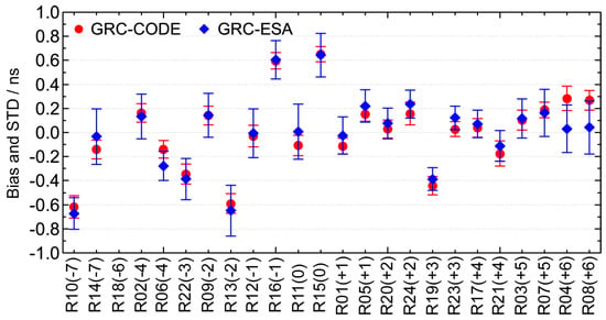
Figure 13.
The bias and STD of the GRC GLONASS satellite P1-P2 DCB estimates, relative to the CODE and ESA for Doy 050–079 in 2014.
The day-to-day scatter (or stability) was the day-to-day variation in the daily DCB estimates, with respect to the monthly mean DCB estimates [44]. The monthly stability of the GPS and GLONASS satellite DCBs, which were determined by the GRC and IAACs, was calculated. The statistics of the monthly stability for the IAACs are presented in Table 3. It was clear that the satellite stability indices were increased greatly in 2014, when compared with those in 2008, because of the increase of the ionosphere variability. The GRC GPS satellite stability was 0.04 ns in 2008 and 0.07 ns in 2014. The GRC GLONASS satellites were less stable than the GPS with a mean value of 0.09 ns in 2014. Although the same ionospheric models were adopted at the GRC, CODE, and ESA, the CODE had the best stability index because of the strategy of using three consecutive days of data, which had increased the smoothness of the DCB estimations [45]. The UPC had the maximum stability index in both 2008 and 2014. The most probable reason was that the DCBs were estimated from the ionospheric code post-fit residuals, after subtracting the slant TEC that was obtained from the GIMs [18]. It was easy to see that the satellite stability for the GRC was comparable to that of the CODE and JPL, and that it was better than the ESA and UPC during both the low and high solar activity periods.
Table 3.
The monthly stability of the GRC and IAACs satellite DCB estimates for Doy 202–231 in 2008 and Doy 050–079 in 2014 (unit: ns).
4.4. GPS and GLONASS Receiver DCBs Validation with IAACs DCBs
The GPS and GLONASS receiver P1-P2 DCBs were compared with the IAACs DCBs in this section. For each comparison experiment, 30 IGS stations with different receiver types were selected. Different from the comparison of the satellite DCB estimates, the receiver DCB estimates were also affected by the geographic latitude because of the ionospheric VTEC latitudinal gradients.
The monthly GPS receiver P1-P2 DCBs for Doy 050–079 in 2014 are presented in Figure 14. The stations with different receiver and antenna types are presented in Table 4. It can be seen that the GPS receiver P1-P2 DCBs ranged from −10.0 to 18.0 ns. The differences between the GRC and IAACs were very small. The receiver DCBs were very similar with the same receiver type, however they also varied with the different antenna types, such as the stations with the receiver ASHTECH UZ-12. The receiver DCBs were nearly the same for the same receiver and antenna type, such as stations SCH2 and CHUR.
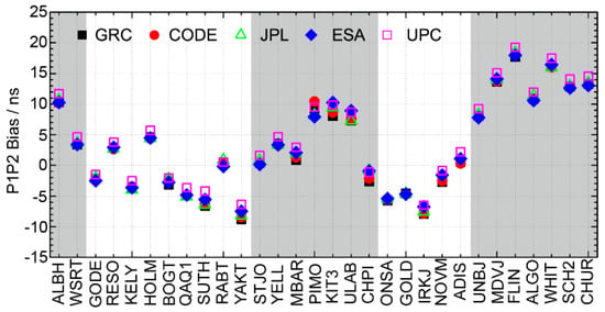
Figure 14.
The GPS receiver P1-P2 DCB estimates of the GRC and IAACs for Doy 050–079 in 2014. The GPS receivers were loosely classified into five types (AOA, ASHTECH, JAVAD, JPS, and TPS).
Table 4.
The stations selected for the GPS receivers’ DCBs comparison for Doy 050–079 in 2014.
Figure 15 shows the monthly GLONASS receiver P1-P2 DCBs for Doy 050–079 in 2014. The four types of receivers are presented in Table 5. Only the CODE and ESA provided the GLONASS receiver DCBs, and the DCBs for GRC agreed well with those for the CODE and ESA. The GLONASS receiver DCBs ranged from −28.0 to 18.0 ns. It was also very clear that the GLONASS receiver DCB estimates were strongly related with the receiver type and antenna type.
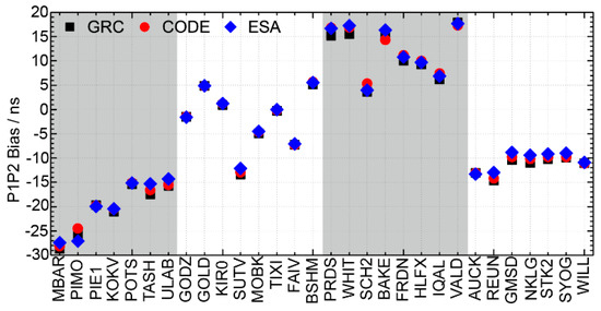
Figure 15.
GLONASS receiver P1-P2 DCB estimates of the GRC, CODE, and ESA for Doy 050–079 in 2014. The GLONASS receivers were classified into four types.
Table 5.
The stations selected for the GLONASS receivers DCBs comparison for Doy 050–079 in 2014.
The mean bias and STD of the GPS receiver P1-P2 DCB estimates for Doy 202–231 in 2008 and Doy 050–079 in 2014 are presented in Figure 16. The stations are listed in the order from the southern latitude to the northern latitude, instead of in the order of the receiver types. Some of the stations were located at low latitude regions, while most of the stations were located at the northern middle and high latitude. It can be seen that the receiver DCB estimates at the GRC were underestimated when compared with the IAACs for most of the stations, both in 2008 and 2014. The biases of the GRC GPS receiver DCB estimates, relative to the IAACs, were within 0.5 ns in 2008. It was increased to 1.0 ns for most of the stations in 2014, except for UPC. The mean biases are presented in Table 6. The STDs of the receiver DCBs differences ranged from 0.05 to 0.30 ns in 2008 and from 0.05 to 1.00 ns in 2014. The STDs increased significantly in 2014, in accordance with those for the satellite DCBs. The STDs at the low latitude were obviously larger than those at the middle and high latitudes. This agreed well with the VTEC STDs in Figure 6, because of the simultaneous estimation of the ionospheric parameters and DCBs. The RMSs of the receiver DCBs differences ranged from 0.06 to 0.76 ns in 2008 and from 0.13 to 2.23 ns in 2014. The mean RMSs were summarized in Table 6.
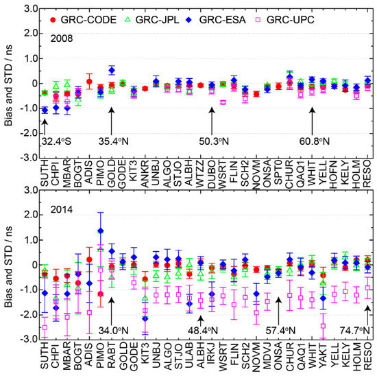
Figure 16.
The bias and STD of the GRC GPS receiver P1-P2 DCB estimates, relative to the IAACs for Doy 202–231 in 2008 (top plot) and Doy 050–079 in 2014 (bottom plot). The receivers are listed in the order of southern latitude to northern latitude.
Table 6.
The bias (before the comma) and RMS (after the comma) of the GRC receiver P1-P2 DCB estimates, relative to the IAACs for Doy 202–231 in 2008 and Doy 050–079 in 2014 (unit: ns).
Figure 17 shows the mean bias and STD of the GLONASS receiver P1-P2 DCB estimates for Doy 050–079, 2014. The GRC GLONASS receiver DCB estimates were also underestimated than the CODE and ESA for most stations. The biases ranged from −2.1 to 1.4 ns and the RMSs ranged from 0.15 to 1.72 ns in 2014. The mean biases and RMSs are also presented in Table 6.
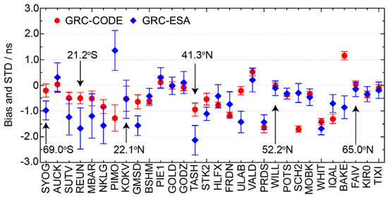
Figure 17.
The bias and STD of the GRC GLONASS receiver P1-P2 DCB estimates, relative to the CODE and ESA for Doy 050–079 in 2014. The receivers are listed in the order of southern latitude to northern latitude.
The monthly stability of the GPS and GLONASS receiver DCBs, which were determined by the GRC and IAACs, are presented in Table 7. The stability of the receiver DCBs was obviously larger than those of the satellite DCBs. The differences in stability between the IAACs were very small for both the GPS and GLONASS. The stability of the receiver DCB estimates, during the high solar activity period, were significantly larger than those during the low solar activity period, which was similar to those for satellite DCBs.
Table 7.
The monthly stability of the GRC and IAACs receiver DCB estimates for Doy 202–231 in 2008 and Doy 050–079 in 2014 (unit: ns).
5. Discussion
Through the above experiments and comparisons, it was demonstrated that the GIMs products that were obtained from the GIMAS software were comparable to those of the CODE, JPL, ESA/ESOC, and UPC. The different techniques and implementations between the GRC and the IAACs are presented in Table 1. The different ionospheric models would have led to great discrepancies at different latitude bands, such as the GRC, JPL, and UPC. However, the different ionospheric strategies had resulted in the maximum STDs at the low latitude, such as the GRC and ESA. However, the accuracies of the GRC VTEC maps were still within the accuracy range of 2–8 TECU for the IGS VTEC products. The systematic biases and STDs of the GRC VTEC maps, relative to the Jason-2 VTEC measurements, also showed similar accuracies to the previous studies. The combination of the ground GNSS data and the altimeter data is expected to improve the accuracies of the VTEC maps over the oceans and the results will be provided soon. The accuracies of the GPS and GLONASS satellite and receiver DCBs were at the same level as the IGS DCB products. The DCBs were mainly related to the performance of the corresponding instruments, of which the GPS satellite DCBs had nearly the same amount from the same block, and the receivers showed similar DCBs with the same receiver type and antenna type. The precisions of the DCBs were affected by the ionosphere models because of the simultaneous estimation method. Based on the GIMAS software, a more precise global ionosphere model was under the testing stage. As a new IAAC member, the GRC of Wuhan University would benefit from the IGS IAACs and would contribute to the global ionosphere mapping and analysis.
6. Conclusions
We modeled the global ionosphere maps and estimated the GPS and GLONASS satellite and receiver DCBs during the low (2008) and high (2014) solar activity periods. The experiments were supported by a new fast computing global ionosphere mapping software, GIMAS, which was developed at the GNSS Research Center of Wuhan University. The performance of the GIMAS-based GIMs was validated with the products of the legacy IGS IAACs (CODE, JPL, ESA/ESOC, and UPC) and the Jason-2 altimeter data.
The results showed that the biases of the GIMAS-based VTEC maps, relative to the IAACs, ranged from −3.0 to 1.0 TECU. The STDs ranged from 0.7 to 1.9 TECU in 2008 and from 2.0 to 8.0 TECU in 2014. Both the biases and STDs at different latitude bands indicated that the strong ionosphere variation at low latitude would increase the complexity of ionosphere modeling and that different ionosphere models or different strategies would lead to significant discrepancies. When the GIMAS-based VTEC maps were compared with the Jason-2 VTEC measurements, a positive systematic bias of about +2.2 TECU in 2014 and a negative systematic bias of about −1.8 TECU in 2008 were observed. The unexpected negative bias suggested that either the GNSS derived VTEC was underestimated or the Jason-2 VTEC was overestimated during the low solar activity period. The STDs was about 2.0 TECU in 2008 and ranged from 2.2 to 8.5 TECU, with respect to the geographic latitude in 2014. The STDs in the Northern Hemisphere were smaller than those in the Southern Hemisphere, because of the denser distribution of stations.
The GPS and GLONASS satellite and receiver P1-P2 DCBs were compared with the IAACs DCBs. The RMSs for the GPS satellites ranged from 0.16 to 0.20 ns in 2008 and from 0.13 to 0.25 ns in 2014, and the RMSs for the GLONASS satellites ranged from 0.26 to 0.31 ns in 2014. The monthly stability of the GPS satellite DCBs was about 0.04 ns (0.07 ns) in 2008 (2014) and that of the GLONASS satellite DCBs was about 0.09 ns in 2014. The GIMAS-based receiver DCBs were underestimated when compared with those of IAACs for most of the stations. The STDs at the low latitude were obviously larger than those at middle and high latitudes, because of the ionosphere variation. The RMSs were 0.21–0.42 ns in 2008 and 0.33–1.47 ns in 2014 for the GPS receivers, and 0.67–0.96 ns in 2014 for the GLONASS receivers. The monthly stability of the GPS receiver DCBs were about 0.16 ns (0.47 ns) in 2008 (2014) and of the GLONASS receiver, the DCBs were 0.48 ns in 2014.
Author Contributions
Q.Zhang and Q.Zhao conceived and designed the experiments; Q.Zhang programmed the GIMAS software and performed the experiments; Q.Zhang wrote the paper; and Q.Zhao provided great help for the revision and modification.
Acknowledgments
We are grateful to the editor and four anonymous reviewers for their helpful suggestions and valuable comments. The research was partially supported by the National Natural Science Foundation of China (Grant Nos. 41574030, 41774035, 41674004). The authors would like to acknowledge the IGS Global Data Center CDDIS for providing the GNSS data. We are thankful to the Center for Orbit Determination in Europe (CODE), the Jet Propulsion Laboratory (JPL), the European Space Operations Center (ESOC) of European Space Agency (ESA), and the Universitat Politècnica de Catalunya (UPC) for providing global ionosphere products. The Centre National d’Etudes Spatiales (CNES) is also greatly acknowledged for providing the Jason-2 products.
Conflicts of Interest
The authors declare no conflict of interest.
References
- Hernández-Pajares, M.; Roma-Dollase, D.; Krankowski, A.; García-Rigo, A.; Orús-Pérez, R. Methodology and consistency of slant and vertical assessments for ionospheric electron content models. J. Geodesy 2017, 91, 1405–1414. [Google Scholar] [CrossRef]
- Mannucci, A.J.; Wilson, B.D.; Yuan, D.N.; Ho, C.H.; Lindqwister, U.J.; Runge, T.F. A global mapping technique for GPS-derived ionospheric total electron content measurements. Radio Sci. 1998, 33, 565–582. [Google Scholar] [CrossRef]
- Feltens, J. The International GPS Service (IGS) Ionosphere Working Group. Adv. Space Res. 2003, 31, 635–644. [Google Scholar] [CrossRef]
- Hernández-Pajares, M.; Juan, J.M.; Sanz, J.; Orus, R.; Garcia-Rigo, A.; Feltens, J.; Komjathy, A.; Schaer, S.C.; Krankowski, A. The IGS VTEC maps: A reliable source of ionospheric information since 1998. J. Geodesy 2009, 83, 263–275. [Google Scholar] [CrossRef]
- Roma-Dollase, D.; Hernández-Pajares, M.; Krankowski, A.; Kotulak, K.; Ghoddousi-Fard, R.; Yuan, Y.; Li, Z.; Zhang, H.; Shi, C.; Wang, C.; et al. Consistency of seven different GNSS global ionospheric mapping techniques during one solar cycle. J. Geodesy 2017, in press. [Google Scholar] [CrossRef]
- Lanyi, G.E.; Roth, T. A comparison of mapped and measured total ionospheric electron content using global positioning system and beacon satellite observations. Radio Sci. 1988, 23, 483–492. [Google Scholar] [CrossRef]
- Davies, K.; Hartmann, G.K. Studying the ionosphere with the Global Positioning System. Radio Sci. 1997, 32, 1695–1703. [Google Scholar] [CrossRef]
- Hernández-Pajares, M.; Juan, J.M.; Sanz, J.; Aragón-Àngel, À.; García-Rigo, A.; Salazar, D.; Escudero, M. The ionosphere: Effects, GPS modeling and the benefits for space geodetic techniques. J. Geodesy 2011, 85, 887–907. [Google Scholar] [CrossRef]
- Liu, J.; Hernandez-Pajares, M.; Liang, X.; An, J.; Wang, Z.; Chen, R.; Sun, W.; Hyyppä, J. Temporal and spatial variations of global ionospheric total electron content under various solar conditions. J. Geodesy 2017, 91, 485–503. [Google Scholar] [CrossRef]
- Schaer, S.; Beutler, G.; Rothacher, M.; Springer, T.A. Daily global ionosphere maps based on GPS carrier phase data routinely produced by the CODE Analysis Center. In Proceedings of the IGS AC Workshop, Silver Spring, MD, USA, 19–21 March 1996; pp. 181–192. [Google Scholar]
- Schaer, S.; Gurtner, W.; Feltens, J. IONEX: The ionosphere map exchange format version 1. In Proceedings of the IGS AC Workshop, Darmstadt, Germany, 9–11 February 1998. [Google Scholar]
- Schaer, S. Mapping and Predicting the Earth’s Ionosphere Using the Global Positioning System; Astronomical Institute, University of Berne: Berne, Switzerland, 1999. [Google Scholar]
- Mannucci, A.J.; Wilson, B.D.; Edwards, C.D. A new method for monitoring the Earth’s ionospheric total electron content using the GPS global network. In Proceedings of the Institute of Navigation GPS-93, Salt Lake City, UT, USA, 22–24 September 1993. [Google Scholar]
- Komjathy, A.; Wilson, B.D.; Runge, T.F.; Boulat, B.M.; Maimucci, A.J.; Reyes, M.J.; Sparks, L.C. A new ionospheric model for wide area differential GPS: The multiple shell approach. In Proceedings of the National Technical Meeting of the Institute of Navigation, San Diego, CA, USA, 28–30 January 2002. [Google Scholar]
- Feltens, J. Development of a new three-dimensional mathematical ionosphere model at European Space Agency/European Space Operations Centre. Space Weather 2007, 5. [Google Scholar] [CrossRef]
- Juan, J.M.; Rius, A.; Hernández-Pajares, M.; Sanz, J. A two-layer model of the ionosphere using Global Positioning System data. Geophys. Res. Lett. 1997, 24, 393–396. [Google Scholar] [CrossRef]
- Hernández-Pajares, M.; Juan, J.M.; Sanz, J. Neural network modeling of the ionospheric electron content at global scale using GPS data. Radio Sci. 1997, 32, 1081–1089. [Google Scholar] [CrossRef]
- Hernández-Pajares, M.; Juan, J.M.; Sanz, J. New approaches in global ionospheric determination using ground GPS data. J. Atmos. Sol.-Terr. Phys. 1999, 61, 1237–1247. [Google Scholar] [CrossRef]
- Hernández-Pajares, M.; Juan, J.M.; Sanz, J.; Solé, J.G. Global observation of the ionospheric electronic response to solar events using ground and LEO GPS data. J. Geophys. Res. Space Phys. 1998, 103, 20789–20796. [Google Scholar] [CrossRef]
- Hernández-Pajares, M.; Juan, J.M.; Sanz, J. Improving the Abel inversion by adding ground GPS data to LEO radio occultations in ionospheric sounding. Geophys. Res Lett. 2000, 27, 2473–2476. [Google Scholar] [CrossRef]
- Li, Z.; Yuan, Y.; Wang, N.; Hernandez-Pajares, M.; Huo, X. SHPTS: Towards a new method for generating precise global ionospheric TEC map based on spherical harmonic and generalized trigonometric series functions. J. Geodesy 2015, 89, 331–345. [Google Scholar] [CrossRef]
- Zhang, H.; Han, W.; Huang, L.; Geng, C.J. Modeling global ionospheric delay with IGS ground-based GNSS observations. Geomat. Inf. Sci. Wuhan Univ. 2012, 37, 1186–1189. (In Chinese) [Google Scholar]
- Zhang, H.; Xu, P.; Han, W.; Ge, M.; Shi, C. Eliminating negative VTEC in global ionosphere maps using inequality-constrained least squares. Adv. Space Res. 2013, 51, 988–1000. [Google Scholar] [CrossRef]
- Dagum, L.; Menon, R. OpenMP: An industry-standard API for shared-memory programming. IEEE Comput. Sci. Eng. 1998, 5, 46–55. [Google Scholar] [CrossRef]
- Zhang, Q.; Zhao, Q.L. Application of parallel computing with OpenMP in global ionosphere mapping. Geomat. Inf. Sci. Wuhan Univ. 2018, 43, 227–233. (In Chinese) [Google Scholar]
- Blewitt, G. An automatic editing algorithm for GPS data. Geophys. Res. Lett. 1990, 17, 199–202. [Google Scholar] [CrossRef]
- Hadas, T.; Krypiak-Gregorczyk, A.; Hernández-Pajares, M.; Kaplon, J.; Paziewski, J.; Wielgosz, P.; Garcia-Rigo, A.; Kazmierski, K.; Sosnica, K.; Kwasniak, D. Impact and implementation of higher-order ionospheric effects on precise GNSS applications. J. Geophys. Res. Solid Earth 2017, 122, 9420–9436. [Google Scholar] [CrossRef]
- Schaer, S.; Beutler, G.; Mervart, L.; Rothacher, M.; Wild, U. Global and regional ionosphere models using the GPS double difference phase observable. In Proceedings of the IGS Workshop, Potsdam, Germany, 15–17 May 1995. [Google Scholar]
- Davies, K. Ionospheric Radio; The Institution of Engineering and Technology: London, UK, 1990. [Google Scholar]
- Mannucci, A.J.; Wilson, B.D.; Yuan, D.N.; Lindqwister, U.J.; Runge, T.F. Global monitoring of ionospheric total electron content using the IGS network. In Proceedings of the IGS Workshop, Potsdam, Germany, 15–17 May 1995. [Google Scholar]
- Emmert, J.T.; Mannucci, A.J.; Mcdonald, S.E.; Vergados, P. Attribution of interminimum changes in global and hemispheric total electron content. J. Geophys. Res. Space Phys. 2017, 122, 2424–2439. [Google Scholar] [CrossRef]
- Afraimovich, E.L.; Astafyeva, E.I.; Oinats, A.V.; Yasukevich, Y.V.; Zhivetiev, I.V. Global electron content: A new conception to track solar activity. Ann. Geophys. 2008, 26, 335–344. [Google Scholar] [CrossRef]
- Dow, J.M.; Neilan, R.E.; Rizos, C. The international GNSS service in a changing landscape of global navigation satellite systems. J. Geodesy 2009, 83, 191–198. [Google Scholar] [CrossRef]
- Azpilicueta, F.; Brunini, C. Analysis of the bias between TOPEX and GPS vTEC determinations. J. Geodesy 2009, 83, 121–127. [Google Scholar] [CrossRef]
- CNES. Jason-3 Products Handbook; SALP-MU-M-OP-16118-CN; CNES: Paris, France, 2016. [Google Scholar]
- Gulyaeva, T.L.; Arikan, F.; Delay, S.H. Scale factor mitigating non-compliance of double-frequency altimeter measurements of the ionospheric electron content over the oceans with GPS-TEC maps. Earth Planets Space 2009, 61, 1103–1109. [Google Scholar] [CrossRef]
- Jee, G.; Schunk, R.W.; Ludger, S. Analysis of TEC data from the TOPEX/Poseidon mission. J. Geophys. Res. Atmos. 2004, 109, A01301. [Google Scholar] [CrossRef]
- Jee, G.; Lee, H.B.; Kim, Y.H.; Chung, J.K.; Cho, J. Assessment of GPS global ionosphere maps (GIM) by comparison between CODE GIM and TOPEX/Jason TEC data: Ionospheric perspective. J. Geophys. Res. Space Phys. 2010, 115, 161–168. [Google Scholar] [CrossRef]
- Orús, R.; Hernández-Pajares, M.; Juan, J.M.; Sanz, J.; Garcıa-Fernández, M. Performance of different TEC models to provide GPS ionospheric corrections. J. Atmos. Sol.-Terr. Phys. 2002, 64, 2055–2062. [Google Scholar] [CrossRef]
- Wilson, B.D.; Mannucci, A.J. Instrumental biases in ionospheric measurements derived from GPS data. In Proceedings of the 6th International Technical Meeting of the Satellite Division of the Institute of Navigation (ION GPS 1993), Salt Lake City, UT, USA, 22–24 September 1993. [Google Scholar]
- Wang, N.; Yuan, Y.; Li, Z.; Montenbruck, O.; Tan, B. Determination of differential code biases with multi-GNSS observations. J. Geodesy 2016, 90, 209–228. [Google Scholar] [CrossRef]
- Hauschild, A.; Montenbruck, O. A study on the dependency of GNSS pseudorange biases on correlator spacing. GPS Solut. 2016, 20, 159–171. [Google Scholar] [CrossRef]
- Montenbruck, O.; Hauschild, A.; Steigenberger, P. Differential code bias estimation using multi-GNSS observations and global ionosphere maps. Navigation 2014, 61, 191–201. [Google Scholar] [CrossRef]
- Li, Z.; Yuan, Y.; Li, H.; Ou, J.; Huo, X. Two-step method for the determination of the differential code biases of COMPASS satellites. J. Geodesy 2012, 86, 1059–1076. [Google Scholar] [CrossRef]
- Dach, R.; Brockmann, E.; Schaer, S.; Beutler, G.; Meindl, M.; Prange, L.; Bock, H.; Jäggi, A.; Ostini, L. GNSS processing at CODE: Status report. J. Geodesy 2009, 83, 353–365. [Google Scholar] [CrossRef]
© 2018 by the authors. Licensee MDPI, Basel, Switzerland. This article is an open access article distributed under the terms and conditions of the Creative Commons Attribution (CC BY) license (http://creativecommons.org/licenses/by/4.0/).