Article

Sewer Inlet Localization in UAV Image Clouds: Improving Performance with Multiview Detection

by
Matthew Moy de Vitry
1,2,*,
Konrad Schindler
2,
Jörg Rieckermann
1 and
João P. Leitão
1
1
Eawag: Swiss Federal Institute of Aquatic Science and Technology, Überlandstrasse 133, 8600 Dübendorf, Switzerland
2
ETHZ: Swiss Federal Institute of Technology Zurich, Wolfgang-Pauli-Strasse 15, 8093 Zurich, Switzerland
*
Author to whom correspondence should be addressed.
Remote Sens. 2018, 10(5), 706; https://doi.org/10.3390/rs10050706
Submission received: 15 March 2018 / Revised: 17 April 2018 / Accepted: 30 April 2018 / Published: 4 May 2018
(This article belongs to the Section Remote Sensing Image Processing)

Abstract

:
Sewer and drainage infrastructure are often not as well catalogued as they should be, considering the immense investment they represent. In this work, we present a fully automatic framework for localizing sewer inlets from image clouds captured from an unmanned aerial vehicle (UAV). The framework exploits the high image overlap of UAV imaging surveys with a multiview approach to improve detection performance. The framework uses a Viola–Jones classifier trained to detect sewer inlets in aerial images with a ground sampling distance of 3–3.5 cm/pixel. The detections are then projected into three-dimensional space where they are clustered and reclassified to discard false positives. The method is evaluated by cross-validating results from an image cloud of 252 UAV images captured over a 0.57-km2 study area with 228 sewer inlets. Compared to an equivalent single-view detector, the multiview approach improves both recall and precision, increasing average precision from 0.65 to 0.73. The source code and case study data are publicly available for reuse.

1. Introduction

1.1. The Need for Urban Drainage Network Infrastructure Data

Urban drainage network infrastructure is foundational to public health and safety in urban areas. As such, great investments have been made into such infrastructure, especially in developed countries. In Switzerland, for example, the replacement value of all public sewer and drainage infrastructure is estimated at 66 billion Swiss francs [1], which corresponds to around 7000 euros per capita. To manage and maintain this infrastructure in the long term, it is essential to catalog the constituent assets and geographical layout of the networks. Comprehensive and detailed network layout information also plays a role when assessing flood risks. According to Hürter and Schmitt [2], the inclusion of sewer inlets in the model has a clear impact on the simulation results for urban pluvial floods caused by medium-sized rain events. This finding speaks against the common engineering practice of considering manholes as the sole interface between surface flows and the drainage network. Going a step further, Simões et al. [3] looked at the impact of capacity restriction of sewer inlets due to debris during flood events. Using a stochastic modeling approach, the authors showed that sewer inlet capacity does indeed have a large impact on flooding occurrence.
Despite these reasons, data pertaining to urban drainage networks are often found lacking, inaccurate, or hard to access. Again in Switzerland, a report from 2012 states that low data availability characterizes the whole water management sector [4]. While no international surveys on the topic are known of, authors from various European countries mention and address the issue of data scarcity in urban drainage [5,6,7]. The main causes for scarcity cited by the authors are a lack of data reporting standards, poor data management practice, lack of coordination between network operations, privacy concerns, and legal constraints. Given that these challenges are not specific to Europe, one can assume that drainage network data scarcity is a general problem in developed urban areas.

1.2. Remote Sensing of Urban Infrastructure

Remote sensing and computer vision offer an automated alternative to expensive and error-prone manual data collection. Most remote sensing methods for small infrastructure found on or near roads are based on data collected at street level. For example, mobile laser scanning has been used to map road inventory such as light poles or manholes [8,9,10], and street-level imagery has been used to map manholes, trees, and telecommunications infrastructure [11,12,13]. In contrast to aerial remote sensing, data collected at street level is often very high resolution and less affected by obstructions such as trees. Furthermore, street-level images are captured with considerable overlap and from multiple perspectives, which can improve detection performance [12,13]. However, precise geographic localization with street-level images can be challenging due to noise in the position and heading information of the images [11]. From the authors’ experience, the positional errors can be up to several meters, which is problematic for small objects like sewer inlets or manholes, which sometimes lie within meters of each other.
Aerial imaging, on the other hand, is very reliable in that respect: high resolution aerial imagery can normally be georeferenced and rectified with submeter accuracy. Though the accuracy of the rectification and georeferencing does depend on the quality of ground control points, this is not usually an issue in urban areas despite strong height relief. This is the case particularly for unmanned aerial vehicle (UAV) imagery, thanks to its very high ground sampling distance (GSD) and large image overlap. While there are no studies of sewer inlet detection in aerial imagery, there have been several that investigate manhole cover detection. From a remote sensing standpoint, manhole covers are similar to sewer inlets in terms of size and construction material. Additionally, the two are related in terms of frequency and location of occurrence. Therefore, it is of value to mention the latest studies in manhole cover detection. Pasquet et al. [14] combined detections from a geometric circle filter with detections from a linear support vector machine (SVM) fed with histogram of oriented gradient (HOG) features. Trained and tested on aerial imagery with a resolution of 4 cm/pixel, the method was able to detect up to 40% of manholes with a precision of 80%. More recently, Commandre et al. [15] implemented and customized a deep convolutional neural network to the task of manhole detection in aerial imagery with a resolution of 5 cm/pixel. Despite the lower resolution, a similar performance is attained. Additionally, they show that a recall of up to 50% can be attained with a precision of 69%. As common in most remote sensing applications, both studies perform detection in single images and do not use multiple views to enhance detection performance.

1.3. Unmanned Aerial Vehicles Enable Low-Cost Collection of Aerial Image Clouds

Unmanned aerial vehicles (UAVs) are natural contenders for multiview aerial detection applications: when UAVs are used for orthoimage creation, aerial images must be captured with a high overlap and processed because of the low flight height and consequently high perspective distortion. In practice, it is recommended to have between 60% and 80% overlap in both lateral and longitudinal directions [16]. To create the orthoimage, the UAV images are undistorted, reprojected with a digital surface model, and stitched together into a single orthoimage using a mosaicking approach. If the end goal is object detection, however, the individual images could also be used directly in a multiview detection framework, as has shown to be successful with ground-level imagery [11,13].

1.4. Scope and Novelty of the Present Study

In this work, we present a multiview framework for detecting small, static objects in UAV image clouds. The framework is applied to the detection of sewer inlets in a municipality near Zurich, Switzerland. The performance of multiview detection is compared to that of an equivalent single-view approach in which objects are detected in an orthoimage of similar resolution and geographical extent as the individual UAV images.
This study is (to the best of our knowledge) the first demonstration of multiview detection with UAV image clouds. From the standpoint of urban water management, while UAVs have been tested for surface imperviousness observation [17] and elevation model generation [18], this study is also the first investigation of UAVs for drainage system inventory mapping. Finally, the detection framework and data presented in this study have been published and free for anyone to reuse or build upon.

2. Methods

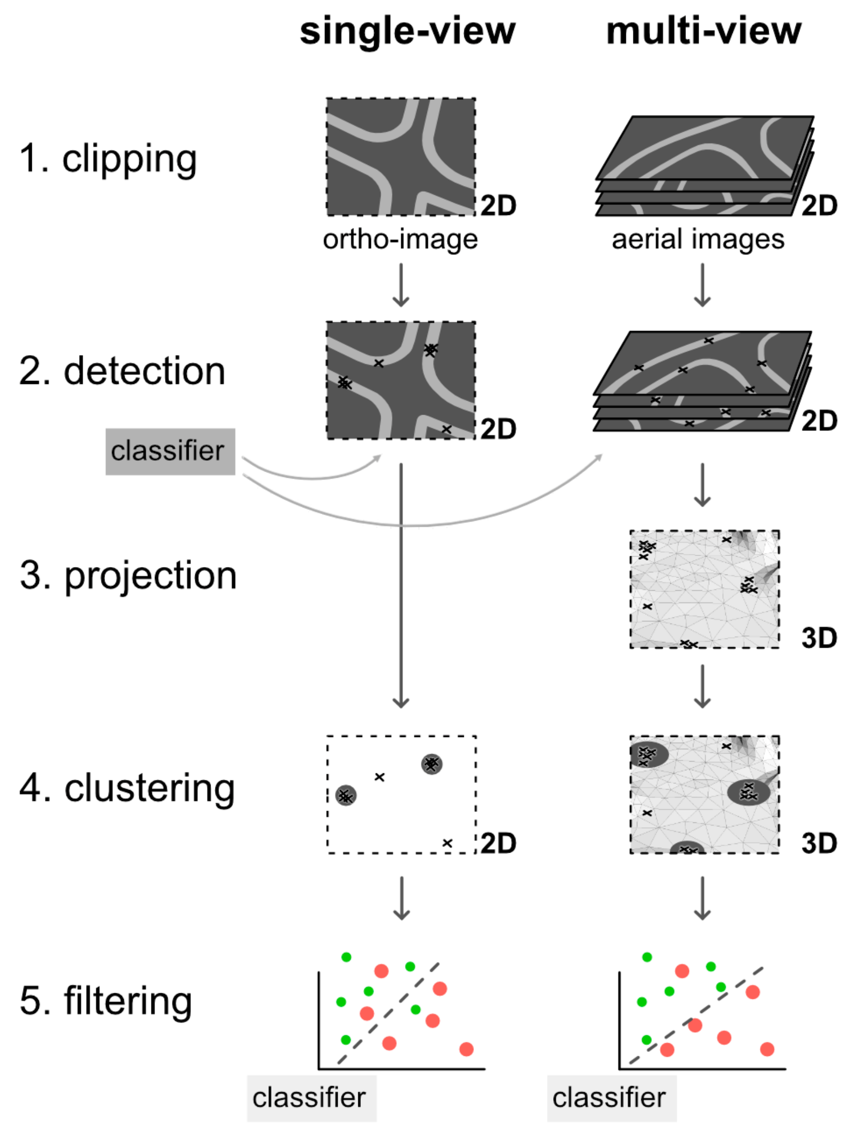
2.1. Single-View and Muliview Detection

The single- and multiview detection approaches compared in this work (Figure 1) differ in essence only in the image medium used for detection: in the first case, objects are detected within a single georeferenced and orthorectified aerial image whereas in the second, individual aerial images are used. There are three main advantages expected from using a multiview approach. Firstly, thanks to the multiple perspectives provided by the individual images, the issue of visual obstruction from trees and moving vehicles should be mitigated. Secondly, the additional information should increase detection accuracy (i.e., fewer false alerts). Finally, the individual UAV images are not processed as is the orthoimage, so a higher image quality and resolution can be expected.
The steps necessary for both approaches are detailed in the following sections and can be summarized follows, as illustrated in Figure 1. In step 1, images are clipped using road network information to limit the search area. In step 2, sewer inlets are detected in each image using a sliding window classifier. In step 3, which only applies to the multiview approach, detections are cast from each image into three-dimensional (3D) space. Overlapping detections are clustered together in step 4, and properties are computed for each cluster. In the final step, the clusters are classified and filtered based on their properties to remove false positives. The detection results are cross-validated in five folds of training and testing data.

2.2. Image Clipping

Sewer inlets are most often situated on the side of the road, and knowledge of this fact can be leveraged to dramatically restrict the area that needs to be searched when localizing sewer inlets, thereby also reducing the number of false positives. In this work, a mask (Figure 2b) was created from land use data, by adding an inner and outer buffer to road edge lines. Since sewer inlets in Switzerland are usually situated on the inner edge of the road and have a principal dimension of around 50 cm, an external buffer of 50 cm and an internal buffer of 100 cm were chosen for the mask. Thus, only image data from the roadsides are retained (Figure 2c) from the original orthoimage (Figure 2a).
While image clipping is trivial for the orthoimage, some processing is required to transform the mask into the projections of the individual (nonrectified) aerial images. First, the mask vertices were enhanced with elevation values extracted from a digital elevation model. Then, the 3D mask was back-projected into the 2D space of each image, using the known camera poses, by back-projecting polygon vertices according to:
v = K R X K R t ,
where v is the point coordinate vector in normalized image space, X is the point coordinate vector in the world coordinate system, K is the [3 × 3] camera lens distortion matrix, R is the [3 × 3] camera rotation matrix, and t is the [3 × 1] camera position vector in the world coordinate system. The K, R, and t camera parameters are determined prior to the detection process using photogrammetry software.
We used the Geospatial Data Abstraction Library (GDAL) and OGR Simple Features Library [19] for reading, writing, and processing geospatial raster and vector data. Numpy [20] was used for matrix operations. Pix4Dmapper [21] was used to estimate camera parameters.

2.3. Object Detection in Images

To detect objects in the images, a sliding window approach is used in conjunction with a cascaded boosted image classifier of the type presented by Viola and Jones [22]. The sliding window approach is a simple way of performing object detection for objects that do not fill the whole image frame. Conceptually, it consists in incrementally sliding a window across the image, classifying the content of the window at each step. The size of the window can be varied according to the range of expected object sized, but in the present work the window size was kept constant since all images are taken from a similar distance to the ground. The method proposed by Viola and Jones is characterized by (i) the concept of integral images, a preprocessing step that accelerates feature computation; (ii) a learning algorithm (Adaboost) that gives weight to discriminative image features among a large pool of candidates; and (iii) a structured decision cascade that discards negative images early in the detection process. The implementation is extremely efficient at detection time despite the sliding window approach because at each window location, features are computed stage by stage. Since the vast majority of proposals are discarded after the first stages, only a fraction of all features need to be computed. This aspect is relevant when many images must be processed, as is the case with multiview detection with hundreds of images. Certain developments have been made since the original implementation by Viola and Jones [22], some of which were found useful for the present work: instead of the originally used features based on Haar basis functions [23], an extended feature set with rotated Haar-like features [24] was used to improve the detection of rotated objects. Also, Gentle Adaboost [25] was used to train the classifier, which is reportedly of greater numerical stability, more resistant to over-fitting and less sensitive to outliers. The same classifier was used for both multiview and single-view approaches.
A feature of sliding window classifiers is that the window slides over the image with a step that is much smaller than the width of the window. Therefore, as the window passes over an object, multiple neighboring detections of the object are documented (Figure 3a–c). Often, these are aggregated directly after detection but in the present study they are aggregated in step 4, after they have been projected into 3D space along with detections from the other images.
OpenCV [26] and specifically the CascadeClassifier class was used as the framework for training and executing the classifier. This class allows the use of different feature sets and boosting methods. The main settings used for training the boosted classifier are listed in Table 1. The number of stages corresponds to the number of successive “strong” classifiers by which an image sample must pass in order to be classified as an object. If any one of the strong classifiers rejects the sample, it is immediately discarded and not evaluated by the following classifiers. This architecture makes it acceptable for each stage to have a moderate false alarm rate, but requires a high hit rate, since the overall performance is estimated as the performance of each stage to the power of the number of stages. Each strong classifier is composed of a number of weak classifiers, which in this study are decision trees of unit depth computed with Extended Haar-like features. The boosting algorithm serves to prioritize training samples from one stage to the next, to help the algorithm identify the most discriminating features for classification. Apart from the feature and boosting type, which were chosen for the reasons explained previously, the other settings were chosen by trial and error as an acceptable compromise between performance and training time.

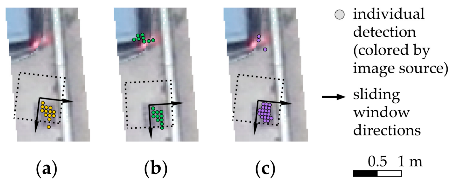
2.4. Projection of Proposals into Three-Dimensional Space

Objects detected in individual UAV images are projected back into world coordinates by casting a ray from the camera projection center into 3D space, i.e.:
X = ( K R ) 1 ( v + K R t )
and intersecting the ray with a digital mesh model of the terrain surface. Because UAV images are captured with a high overlap, each sewer inlet can be detected in multiple images, which leads to clusters of points around the actual sewer inlet locations (Figure 4a). This is accentuated by the fact that in each image, sewer inlets are detected multiple times due to the sliding window. Intersections are computed with the Visualization Toolkit (VTK) Library [28] that internally implements OBBTree [29], a data structure for efficiently detecting interference between geometries.

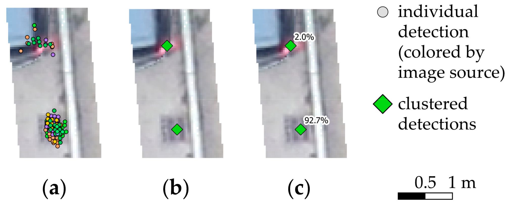
2.5. Clustering Proposals

We use the Density-Based Spatial Clustering for Applications with Noise (DBSCAN) algorithm [30] for identifying clusters (Figure 4b). The algorithm identifies clusters based on a minimum density threshold set by the user, where the density threshold is roughly defined by a minimum number of points within a given area. DBSCAN is well-suited to the sewer inlet detection problem because it scales well with large numbers of points and clusters. Additionally, the points are clustered in 3D space, which is useful if elevation needs to be accounted for. However, the algorithm is sensitive to the density threshold set by the user. In this work, the threshold was adjusted with a simple grid search, based on the typical sewer inlet area of around 0.25 m2 and the expected image overlap. Different clustering parameters were used for single-view detection. The clustering is performed with the scikit-learn Python package [31].

2.6. Removal of False Positives Based on Cluster Properties

The clusters of individual detections are characterized and classified in order to remove false positives. For each cluster, the following properties are computed:
  • Detection count: the number of detections that are part of the cluster.
  • Image count: the number of images contributing detections to the cluster.
  • Maximum, average, and summed detection scores: each of the detections comes with a score from last stage of the Viola–Jones classifier. For the ensemble of detections belonging to a cluster, the maximum score is found, and the arithmetic average and the sum of the scores are computed.
  • Surface area: the surface area of the bounding box containing the detections is computed in map units. This property informs on how spread out the detections are.
  • Density: the density is computed as the number of detections divided by the surface area.
  • Histogram of detections per image: a vector x, with each element x i containing the number of UAV images contributing i detections to the cluster, with i varying from 1 to 49. The vector is generally quite sparse.
  • Average and maximum detections per image: for images contributing detections to the cluster, the average and maximum number of detections is computed.
These properties are used as features to predict whether the object candidate actually corresponded to a sewer inlet. This is a typical two-class classification problem for which we tested three established classification algorithms: Linear SVM, Logistic Regression (LR), and Artificial Neural Network (ANN). With SVM, a hyperplane is fitted in between the two classes of data such that the margin between the data and hyperplane are maximized. SVM are not well suited to nonseparable classes of data and by default do not provide confidence scores for predictions. However, it is possible to estimate confidence scores using Platt scaling [32], with n-fold cross-validation to avoid overfitting the scaling parameters. With LR, a logistic curve is fitted to the data by maximizing the likelihood of observing the data. In contrast to SVM, LR does not assume that the classes are separable and the predictions provided by LR have a direct probabilistic interpretation. In this work, the ANN used is a multilayer perceptron (MLP) with a single hidden layer with 100 neurons. The MLP is trained by adjusting the connection weights between neurons to minimize prediction error. ANN are valuable when the boundary between classes is non-linear. As with LR, the output of ANN is given in terms of confidence scores. Thanks to these classification methods, each cluster can be assigned a confidence scores0F, as illustrated in Figure 4c. For the details of these methods, we refer to standard textbooks such as [33,34]. Since multiview clusters have fundamentally different properties due to the additional information they contain, the cluster classifier must be trained for single-view and multiview clusters separately. In all cases, classification was performed with the scikit-learn Python package [31].

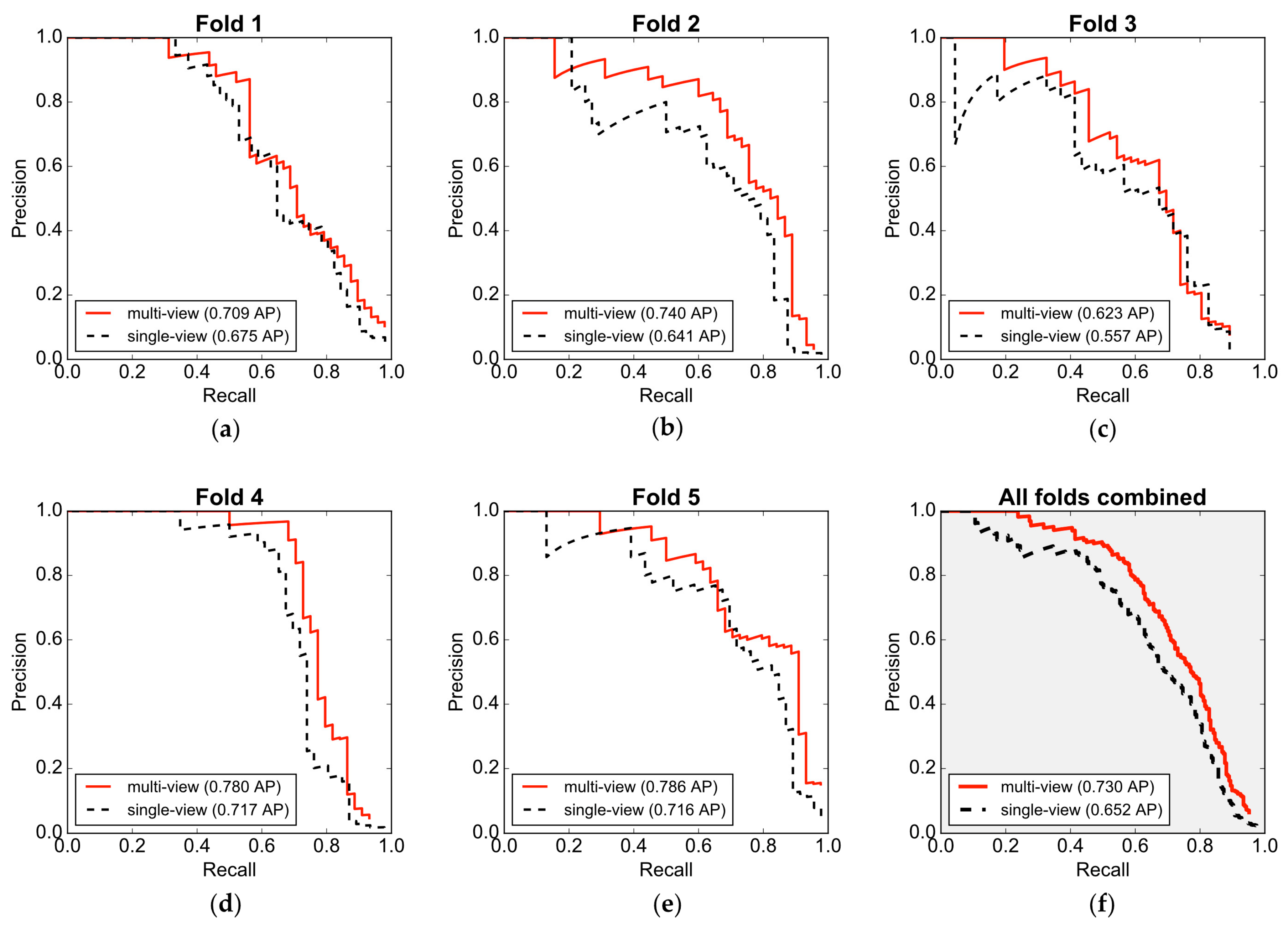
2.7. Assessing Detection Performance

Both the multiview and the single-view detection methods that were implemented provide point detections and not bounding boxes, as is otherwise often the case for object detection. It was therefore not possible to use, for example, the intersection-over-union ratio to evaluate whether an object was matched. Instead, since the representative object size is assumed to be of around 50 cm, an object was considered matched to a cluster if the centers of the two are situated within 50 cm of each other.
The cluster classification step described in the previous section assigns to each cluster a confidence score based on the cluster’s properties. By increasing the confidence threshold for accepting a cluster as an object, the classification is made more conservative (fewer false positives but also fewer true positives). To measure this tradeoff, we use the well-known precision and recall metrics:
P r e c i s i o n = t r u e   p o s i t i v e s t r u e   p o s i t i v e s + f a l s e   p o s i t i v e s
R e c a l l = t r u e   p o s i t i v e s t r u e   p o s i t i v e s + t r u e   n e g a t i v e s
Both precision and recall can take values between 0 and 1, where a low precision means many false positives and a low recall means many objects were missed. Precision and recall are often computed for a range of confidence intervals between 0 and 1, and plotted against each other in a precision-recall curve. The shape of the precision-recall curve can be summarized by the average precision (AP), which corresponds to the area below the curve:
A P = n ( R e c a l l n R e c a l l n 1 ) * P r e c i s i o n n
where n designates the n-th probability threshold for which precision and recall are computed. Perfect classification yields an AP of 1, and the chance level is an AP of 0.5, given a balanced number of positive and negative samples. Object detection problems, however, are not balanced since there are practically infinite negative samples, therefore the actual chance level is much closer to zero.
To assess whether the performance of the multiview localization is statistically different from that of the single-view localization, we perform a paired difference t-test on the AP of the cross-validation folds. Student’s t-test is a statistical test commonly used to verify whether two sets of data are significantly different. It assumes that both sets of data follow a normal distribution of unknown standard deviations. The pairing eliminates confounding effects due to differences between folds, thereby increasing the statistical power of the test. First, we must compute the difference A P i between the multiview and single-view AP of each fold:
A P i =   A P i m u l t i v i e w A P i s i n g l e v i e w
where i stands for the fold index, taking values between 1 and the number of folds n . Under these conditions, the test value t is then computed as:
t =   X ¯ D μ 0 s D n
where X ¯ D and s D are the mean and standard deviation of the differences A P i , n is the number of folds, and μ 0 is equal to zero under the null hypothesis that the multi- and single-view deliver the same performance.

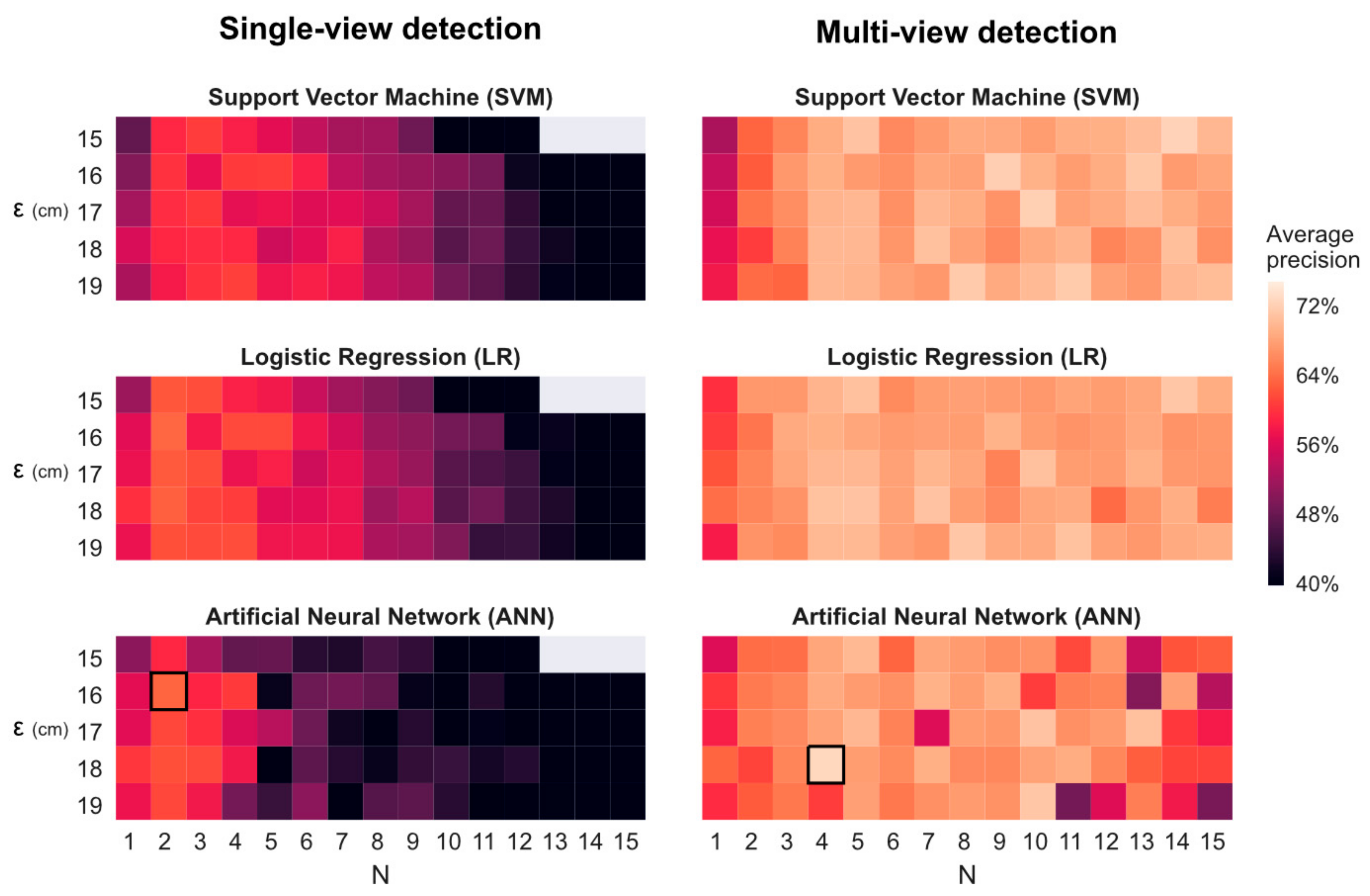
2.8. Analyzing Sensitivity to Clustering Parameters

The clustering algorithm used in this work, DBSCAN [30], is known to be sensitive to the two parameters that define minimum cluster core density. To elucidate the influence of these parameters, we conducted a sensitivity analysis by varying the two parameters: (i) ε is the maximum cluster core size and should be chosen according to object size and localization accuracy, and (ii) N is the minimum number of points that should be found within the cluster core. N depends on how the sliding window iterates over the images and on the number UAV images in which each object is visible. These two parameters ε and N were varied on a grid between values of 0.15–0.25 m and 1–15 samples, respectively1F. These ranges were selected based on a preliminary sensitivity analysis that was broader and coarser than the one presented in the results.
For each combination of parameter values, both the single-view and multiview detections were clustered and classified using the three classifiers (SVM, LR and ANN). The quality of the resulting clusters is measured by means of the average precision (AP), and differentiated by the cluster classification algorithm used.

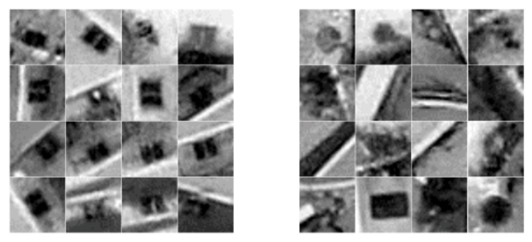
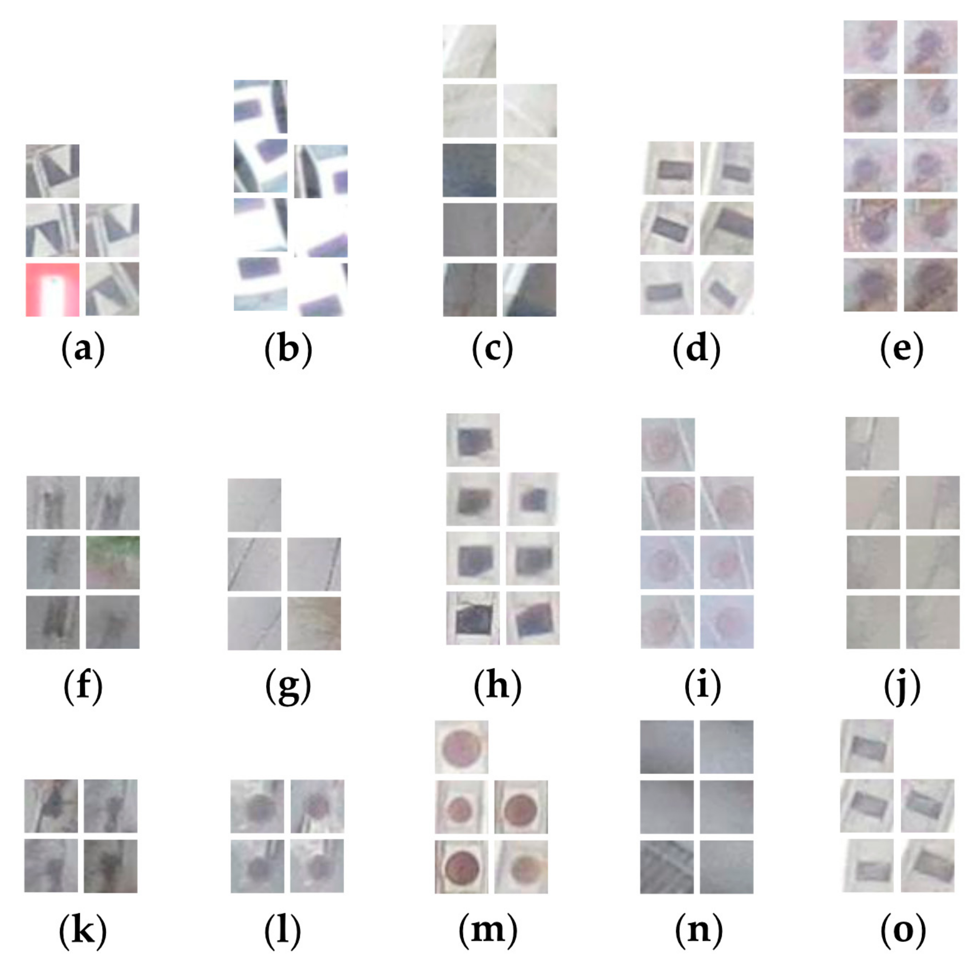
2.9. Analyzing Hard Negatives

Hard negatives, which are detection errors committed with high confidence by the classifier, offer insight into the shortcomings of the method and potential paths for improvement. However, such an analysis remains fundamentally qualitative since the actual underlying causes of detection errors can only be presumed based on visual inspection of the images. In the present analysis, the 15 highest-scoring false positives and 15 lowest-scoring false negatives are extracted and their causes for misclassification are hypothesized. The causes are then ranked according to frequency of occurrence.

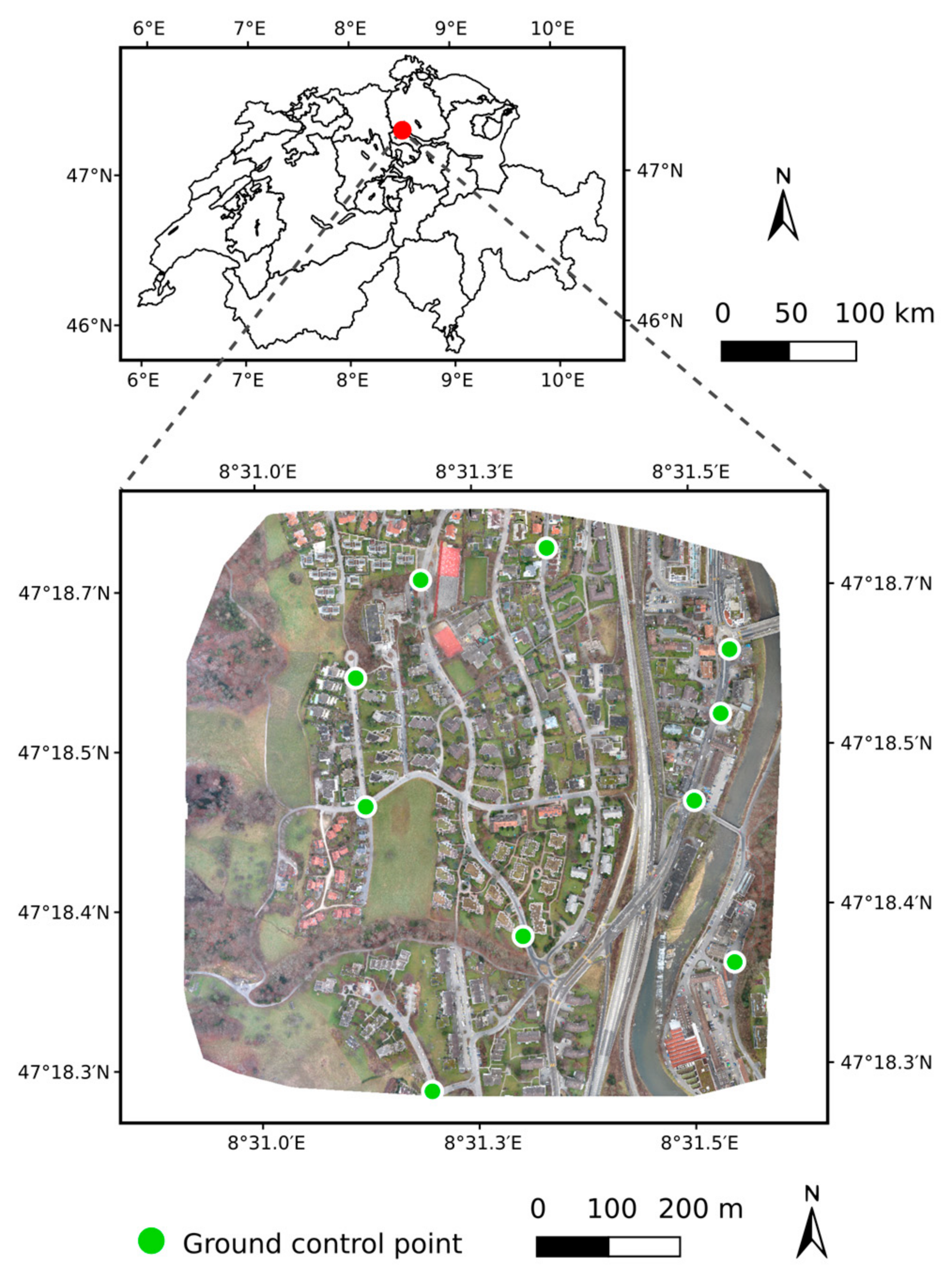
3. Study Area and Data Sets

3.1. Data Collection and Preprocessing

The UAV used to collect data in this study is a fully autonomous electric fixed-wing UAV, the eBee (1st generation) produced by senseFly SA (Cheseaux-sur-Lausanne, Switzerland). With a foam body, a wingspan just under one meter, and a rear-facing propeller, it is safe and well-suited to urban or suburban areas. The UAV carries a 16 MP Canon IXUS 125 HS compact digital camera that is controlled by the UAV autopilot. At typical cruise heights of 100 to 300 m, GSD of the images is between 3 and 10 cm/pixel. The UAV was flown over a residential area near Zurich, Switzerland, in conformity to the Swiss regulations for special category aircraft [35]. These regulations allow autonomous flight without a special license or permit under the following conditions: manual, line-of-sight flight override must be possible at all times; flight must be specified distances away from certain protected nature areas, military facilities, gatherings of people, airports, landing strips, and heliports; for airplanes heavier than 500 grams, a liability insurance of at least 1 million Swiss francs is needed; privacy and data protection laws must be respected. In total, 252 images were taken at a flight height of 90 m, giving a GSD of 3–3.5 cm/pixel (due to variations in perspective and topography). In the study area, 228 sewer inlets were identified manually in the UAV images (Table 2).
The UAV images were processed with Pix4Dmapper [21] to estimate internal and external camera parameters and generate an orthoimage (Figure 5) as well as a digital surface model (DSM) for the case study. The orthoimage is created by making a mosaic from projections of the UAV images, during which resolution is slightly reduced. While minimal loss of image quality is experienced for flat horizontal surfaces (like roads), objects with sharp or complex edges (like buildings) can suffer from distortions and artefacts. These issues are generally of no concern for sewer inlet detection, unless such an object is situated over or right next to a sewer inlet. Ten ground control points were used to georeference the project (placement shown in Figure 5, registration error documented in Table A1). The processing time for estimating camera parameters was 7 min, and the subsequent processing time for generating the orthoimage and DSM was 3 h (using an Intel i7-4790K CPU @ 4 GHz, with 16 GB RAM and a 12 GB NVIDIA GeForce GTX TITAN X graphics card).

3.2. Training and Testing Data

The same case study area was used both for training and testing the detection methods. Because of the limited number of objects contained within the area, we cross-validate the results with five folds of train (80%) and test (20%) data. In each fold, the objects labeled for training were used to extract positive training images from the UAV images (resulting in multiple images/views per object). Negative training images were extracted from locations taken from the highest scoring hard negatives from previous detection runs. The positive and negative sample images were then transformed to greyscale and augmented with random rotations and reflections (positive samples were augmented by a factor 3 and negative samples by a factor 2). The final images were of 32 × 32 pixel resolution, some of which are shown in Figure 6. To train the Viola–Jones classifier, 2661 positive and 3936 negative samples were used.
For training the cluster classifier, the clusters were first divided into three categories: (i) clusters that match to objects labeled for training (training positives); (ii) clusters that match to objects labeled for testing (testing positives); and (iii) clusters that do not match to an object (false positives). Of the false positives, 80% were randomly selected to be used for classifier training, along with the training positives. The remaining 20% were combined with the testing positives to form a test set.

4. Results

4.1. Multiview Significantlys Outperforms Single-View Detection

In Figure 7, the precision-recall curves of the best multiview detector (red) are compared with those of the best single-view detector (black). Both detectors use ANN for cluster classification, but are optimal with different clustering parameters, as illustrated in Figure 8. The comparison is made for each fold of test data (Figure 7a–e), as well as for all test data combined (Figure 7f). The results show that in terms of average precision, the multiview approach precision is improved consistently across all folds of data. Using the paired t-test described in Section 2.7, we obtain a t score of 7.2 standard errors, corresponding to a p-value of 0.002 for a two-tailed test, which is significant at p < 0.01. Overall, average precision for the combined test data is increased from 0.652 to 0.730 (Figure 7f), which is a relative increase of about 12%.

4.2. Sensitivity to Clustering Algorithm Parameters

The results of the clustering parameter sensitivity analysis (Figure 8) show that overall, multiview detection performs better than single-view detection regardless of the cluster classification algorithm. Additionally, multiview detection is less sensitive to clustering parameters than single-view detection, as can be seen in the broad color gradient of the single-view results. While SVM, LR, and ANN all perform comparably, ANN was able to produce detections with the highest average precision for both approaches.
For single-view detection (Figure 8), optimal clustering parameter values are situated around N = 2 and ε = 16. The low value of N is expected, since there is only one image in which objects can be detected. For multiview detection, performance is best for N values above N = 3, after which there is no clear dependency on clustering parameters except for the ANN, for which performance begins to degrade at N = 11.

4.3. Analysis of Nature of Hard Negatives

In Figure 9, the 15 highest-scoring locations falsely classified as sewer inlets are shown. In this sample, the main reasons for false detection are apparently (i) geometric patterns on the ground with high contrast (7 cases); (ii) manholes or round sewer inlets (4 cases). For the remaining four cases, no clear reason can be identified.
In Figure 10, the 15 sewer inlets with the lowest detection scores are shown. The following reasons may have caused them to not detected: (i) insufficient image quality or obstruction (6 cases); (ii) too few images in which the sewer inlet is visible (5 cases); (iii) they are visually different from typical inlets used for training (5 cases); (iv) the object surroundings are complex or unusual (2 cases); or (v) the image pose or DSM is imprecise (1 case).

5. Discussion

5.1. Comparison to Previous Work

As stated earlier, there are no studies to our knowledge investigating sewer inlet identification in aerial images, let alone in UAV image clouds. If compared to recent work on manhole cover detection in aerial imagery, which is a similar problem, our results are 15–20 percentage points better in terms of precision. At 40% recall, Pasquet et al. [14] report 80% precision (we achieve 95% precision) and at 50% recall, Commandre et al. [15] report 69% precision (we achieve 90% precision). Besides the use of a multiview approach, there are two other aspects of our study that could give an edge, namely the slightly higher image resolution used and the preliminary image-clipping step. The differences between the two detection subjects must also be stated: sewer inlets are smaller than manholes, but they also have visual patterns with higher contrast than manholes.

5.2. Advantages of Multiview Detection

While the performance increase thanks to multiview detection is significant, it is not exceptionally large as compared to single-view detection (Figure 7). One could have expected the multiview approach to greatly improve detection performance, especially for difficult-to-detect objects (e.g., partially hidden by nearby obstacles) since the multiview approach provides information from many angles of view as compared to the single-view approach. However, this phenomenon, which would translate to higher performance on the right side of the precision-recall curve, is not marked. One possible explanation is that since the images were taken vertically (configured to 0° from nadir), the difference in perspective was not sufficient to make a strong difference for detection. Another explanation is that there were simply not many objects hidden from view in such a way (e.g., vegetation is not a major issue because of the winter season of the flights).

5.3. Sensitivity to Clustering Parameters

The sensitivity analysis (Figure 8) reveals another advantage of multiview detection, which is that it is less sensitive to clustering parameters than single-view detection. Thus, when applying the method to new locations, there is a greater chance that the clustering parameters identified in this study function well, despite inevitable differences in the data.
For both approaches, there is some noise in the performance level, particularly for the ANN cluster classifiers. This noise can be explained by the stochastic and iterative nature of classifier optimization algorithms, which due to high class overlap sometimes fail to reach the global optimum. In practice, the noise may be a disadvantage if one desires to identify optimal parameter values.

5.4. Role of Digital Surface Model Accuracy

While not investigated in this work, the accuracy of the DSM used to project detections into 3D space can affect detection results. Indeed, if the surface model is inaccurate in the proximity of a sewer inlet, then the projected detections (as in Figure 3) will be erroneous and cause the resulting cluster of points (as in Figure 4) to be more dispersed and possibly shifted. Due to the fact that road surfaces are relatively flat and can be well-described with UAV photogrammetry [18], DSM accuracy is not expected to be a major factor of error in the present study. Indeed, in the analysis of hard negatives, only one of 15 sewer inlets appeared to suffer from localization issues (Figure 10f).

5.5. Improvement Potential and Directions for Future Work

The results presented in this work could possibly be improved upon if certain changes were made to the data collection and methodology. The analysis of hard negatives revealed that some of the main reasons for error, namely high contrast patterns on the ground and unusual sewer inlet shapes, could be solved by increasing the amount and diversity of training data. Other causes of error, namely differentiating manholes from round sewer inlets and low image quality, could be solved by increasing image quality (e.g., by flying lower or using a better camera). The problem of obstruction by vegetation could be mitigated by increasing the tilt angle at which images are taken. In terms of the method, improvements could be made by applying deep convolutional neural networks (DCNN) instead of Viola–Jones. DCNNs, such as Faster R-CNN [36] (a combined region proposal and convolutional neural network), are currently state-of-the-art for most object detection challenges, although they are computationally expensive and require much training data. It is also questionable whether current DCNNs are well suited to small objects like sewer inlets, which have little internal structure [37]. Another change that could be made to the methodology can be illustrated by the failure cases in Figure 10k–o. In these examples, which are probably at the edges of the study area, only one to four images are able to see the sewer inlets. However, the current cluster properties do not account for the visibility of a sewer inlet—thereby penalizing objects in areas where images are less frequent or where obstructions block the view. Finally, sewer inlets, like most public infrastructure objects, have typical distributions (e.g., one manhole every 20 m and rarely two manholes next to each other). While these patterns are regional, they are often known a priori and could be taken into account in the cluster classification process.

5.6. Inherent Limitations of Aerial Sewer Inlet Mapping

Despite the many possibilities for improvement, there are two main limitations that are intrinsic to the approach of automated aerial sewer inlet localization. First, there is an unavoidable risk that a portion of the objects are not visible in aerial images because they are momentarily covered by vehicles or debris. This risk can be partially mitigated by performing multiple flights, at different times of day and different seasons in the year. Second, there is a large variety in the form and situation of sewer inlets, with some being integrated into the curbstone. To accommodate for this variety, one must not only increase the variety within the training data, but also adapt how images are captured, e.g., by further increasing camera tilt. Therefore, depending on the completeness required of the data and the relevance of the aforementioned limitations, it may be necessary to adjust the detection method or to manually verify the detection results.

5.7. Practical Considerations for Urban Water Management

As stated in the introduction, we understand the scarcity of urban drainage infrastructure to be widespread. Even when urban drainage asset managers hold a catalog of assets, it is common that this catalog is incomplete or outdated when it comes to sewer inlets. Based on our experience with establishing the case study ground truth for the present study, for which no reliable ground truth was originally available, having a pool of proposals greatly improves the speed and accuracy of manual object localization. In this context, the primary application of the UAV-sourced data would be to suggest likely sewer inlet locations, and therefore the classifier confidence threshold should be selected to favor data completeness (i.e., recall) over precision. The proposals can then be manually validated to update the inventory. In practice, this can be done in the form of a dedicated field survey or integrated into the routine tasks of municipal workers (e.g., street sweeping or sewer inlet cleaning). In cases where street-level imagery is available, objects can also be validated remotely.
Thanks to the flexibility of UAV-based data collection, such an inventory update would probably benefit from multiple data collection campaigns, e.g., in winter (low vegetation cover), under different lighting conditions, and to randomize the visibility of obstructions such as parked cars). In the context of operational urban water management, regular UAV flights would also be of value for detecting blockages and scheduling maintenance. Based on the results of [38], such an application would reduce the risk of urban pluvial flooding.

5.8. Reusability and Generality of the Multiview Methodology

Although the methodology described in this work is presented in the context of urban drainage infrastructure mapping, using sewer inlets as a case study and a UAV as a platform for image capture, it is in fact of general applicability. Still within the context of infrastructure mapping, one could apply the methodology to manhole covers, rainwater tanks, or power transformers. In the realm of environmental research, it is applicable to the detection of plant species or animal nests. Even in the context of medical science and dermatology, with only slight adaptation it could be turned into a tool for identifying birth marks and moles.

6. Conclusions

This work demonstrates that the use of a multiview framework significantly improves the detection performance for sewer inlets from UAV imagery. With a cross-validated case study with 228 sewer inlets, we show that the use of additional image information increases average precision from 0.652 to 0.730 as compared to an equivalently trained single-view detector. The gain is attributed not only to the additional perspectives made available, but also to the ability to exploit the full resolution of the raw UAV images. The multiview approach is further able to identify 60% of the sewer inlets with a precision of 80% and localize them in three dimensions. Both precision and recall are substantially better than the latest reported results for the comparable problem of manhole cover detection. For urban water practitioners seeking to create or update their inventory, the value added by multiview detection is more than the incremental improvement that is usually gained by tuning the image classification method. Thus, this sewer inlet detection solution can be used to address the frequently mentioned scarcity of urban drainage infrastructure data. The methodology, for which the code has been released, can easily be adapted for reuse within other infrastructure or environmental mapping projects.

Supplementary Materials

The data used in this paper is available online at https://zenodo.org/record/1197592, and the code is available online at https://github.com/Eawag-SWW/raycast.

Author Contributions

M.M.d.V. collected the data, processed the data, and drafted the manuscript. K.S. provided essential support for designing and implementing the object detection methods. J.P.L. and J.R were principle investigators of the project, providing valuable support in the orientation and coordination of project execution, and paper drafting. All authors were involved in editing and reviewing the manuscript.

Acknowledgments

This project was financed by the Swiss National Science Foundation under grant #169630. We thank Peter M. Bach for proofreading the manuscript. We thank the anonymous reviewers for their insightful comments and suggestions, which helped improve the paper.

Conflicts of Interest

The authors declare no conflicts of interest. The founding sponsors had no role in the design of the study; in the collection, analyses, or interpretation of data; in the writing of the manuscript, and in the decision to publish the results.

Appendix

Table A1. Coregistration error of orthoimage and DSM estimated at ground control points.
GCP NameError X (m)Error Y (m)Error Z (m)
E0.006−0.025−0.029
F0.0230.016−0.007
H−0.0170.033−0.003
G0.0100.0270.013
D0.014−0.000−0.024
J−0.0190.0130.000
C0.0010.004−0.064
A−0.008−0.009−0.006
I−0.011−0.0240.002
B0.004−0.0220.059
Mean (m)0.0003320.001385−0.005928
Sigma (m)0.0132050.0199850.029818
RMS Error (m)0.0132090.0200330.030401

References

  1. Verband der Schweizerischen Abwasser- und Gewässerschutzfachleute (VSA). Kosten und Leistungen der Abwasserentsorgung—Erhebung 2010; VSA: Glattbrugg, Switzerland, 2011. (In German) [Google Scholar]
  2. Hürter, H.; Schmitt, T.G. Die bunte Welt der Gefahrenkarten bei Starkregen—Ein Methodenvergleich. Proceedings of Aqua Urbanica 2016, Rigi-Kaltbad, Switzerland, 26–27 September 2016; pp. 1–5. (In German). [Google Scholar]
  3. Simões, N.E.; Ochoa-Rodríguez, S.; Wang, L.-P.; Pina, R.D.; Marques, A.S.; Onof, C.; Leitão, J.P. Stochastic Urban Pluvial Flood Hazard Maps Based upon a Spatial-Temporal Rainfall Generator. Water 2015, 7, 3396–3406. [Google Scholar] [CrossRef] [Green Version]
  4. Maurer, M.; Chawla, F.; von Horn, J.; Staufer, P. Abwasserentsorgung 2025 in der Schweiz; Schriftenreihe der Eawag: Dübendorf, Switzerland, 2012. (In German) [Google Scholar]
  5. Mair, M.; Zischg, J.; Rauch, W.; Sitzenfrei, R. Where to Find Water Pipes and Sewers?—On the Correlation of Infrastructure Networks in the Urban Environment. Water 2017, 9, 146. [Google Scholar] [CrossRef]
  6. Blumensaat, F.; Wolfram, M.; Krebs, P. Sewer model development under minimum data requirements. Environ. Earth Sci. 2012, 65, 1427–1437. [Google Scholar] [CrossRef]
  7. Commandré, B.; Chahinian, N.; Bailly, J.S.; Chaumont, M.; Subsol, G.; Rodriguez, F.; Derras, M.; Deruelle, L.; Delenne, C. Automatic reconstruction of urban wastewater and stormwater networks based on uncertain manhole cover locations. In Proceedings of the 14th IWA/IAHR International Conference on Urban Drainage (ICUD 2017), Prague, Czech Republic, 10–15 September 2017. [Google Scholar]
  8. Yu, Y.; Li, J.; Guan, H.; Wang, C.; Yu, J. Automated detection of road manhole and sewer well covers from mobile LiDAR point clouds. IEEE Geosci. Remote Sens. Lett. 2014, 11, 1549–1553. [Google Scholar] [CrossRef]
  9. Yu, Y.; Li, J.; Guan, H.; Wang, C.; Yu, J. Semiautomated Extraction of Street Light Poles From Mobile LiDAR Point-Clouds. IEEE Trans. Geosci. Remote Sens. 2015, 53, 1374–1386. [Google Scholar] [CrossRef]
  10. Pu, S.; Rutzinger, M.; Vosselman, G.; Oude Elberink, S. Recognizing basic structures from mobile laser scanning data for road inventory studies. ISPRS J. Photogramm. Remote Sens. 2011, 66, S28–S39. [Google Scholar] [CrossRef]
  11. Wegner, J.D.; Branson, S.; Hall, D.; Schindler, K.; Perona, P. Cataloging Public Objects Using Aerial and Street-Level Images—Urban Trees. In Proceedings of the 2016 IEEE Conference on Computer Vision and Pattern Recognition (CVPR), Las Vegas, NV, 26 June–1 July 2016; IEEE: New York, NY, USA, 2016; pp. 6014–6023. [Google Scholar]
  12. Hebbalaguppe, R.; Garg, G.; Hassan, E.; Ghosh, H.; Verma, A. Telecom Inventory Management via Object Recognition and Localisation on Google Street View Images. In Proceedings of the 2017 IEEE Winter Conference on Applications of Computer Vision (WACV), Santa Rosa, CA, USA, 24–31 March 2017; IEEE: New York, NY, USA, 2017; pp. 725–733. [Google Scholar]
  13. Timofte, R.; Van Gool, L. Multi-view manhole detection, recognition, and 3D localisation. In Proceedings of the 2011 IEEE International Conference on Computer Vision Workshops (ICCV Workshops), Barcelona, Spain, 6–13 November 2011; IEEE: New York, NY, USA, 2011; pp. 188–195. [Google Scholar]
  14. Pasquet, J.; Desert, T.; Bartoli, O.; Chaumont, M.; Delenne, C.; Subsol, G.; Derras, M.; Chahinian, N. Detection of Manhole Covers in High-Resolution Aerial Images of Urban Areas by Combining Two Methods. IEEE J. Sel. Top. Appl. Earth Obs. Remote Sens. 2016, 9, 1802–1807. [Google Scholar] [CrossRef]
  15. Commandre, B.; En-Nejjary, D.; Pibre, L.; Chaumont, M.; Delenne, C.; Chahinian, N. Manhole Cover Localization in Aerial Images with a Deep Learning Approach. ISPRS Int. Arch. Photogramm. Remote Sens. Spat. Inf. Sci. 2017, 42, 333–338. [Google Scholar] [CrossRef]
  16. Ortega, M.; Jesse, J.; Gkintzou, C. Pix4D Support Team Pix4D Knowledge Base. Available online: https://support.pix4d.com/entries/26825498 (accessed on 18 June 2014).
  17. Tokarczyk, P.; Leitao, J.P.; Rieckermann, J.; Schindler, K.; Blumensaat, F. High-quality observation of surface imperviousness for urban runoff modelling using UAV imagery. Hydrol. Earth Syst. Sci. 2015, 19, 4215–4228. [Google Scholar] [CrossRef]
  18. Leitão, J.P.; Moy De Vitry, M.; Scheidegger, A.; Rieckermann, J. Assessing the quality of digital elevation models obtained from mini unmanned aerial vehicles for overland flow modelling in urban areas. Hydrol. Earth Syst. Sci. 2016, 20, 1637–1653. [Google Scholar] [CrossRef]
  19. Warmerdam, F. The Geospatial Data Abstraction Library. In Open Source Approaches in Spatial Data Handling; Hall, G.B., Leahy, M.G., Eds.; Springer: Berlin/Heidelberg, Germany, 2008; Volume 2, pp. 87–104. [Google Scholar]
  20. Van der Walt, S.; Colbert, S.C.; Varoquaux, G. The NumPy Array: A Struture for Efficient Numerical Computation. Comput. Sci. Eng. 2011, 13, 22–30. [Google Scholar] [CrossRef]
  21. Pix4D Developers Pix4Dmapper Software Manual. Available online: https://support.pix4d.com/entries/28216826 (accessed on 17 June 2014).
  22. Viola, P.; Jones, M. Rapid object detection using a boosted cascade of simple features. In Proceedings of the 2001 IEEE Computer Society Conference on Computer Vision and Pattern Recognition (CVPR 2001), Kauai, HI, USA, 8–14 December 2001; IEEE: New York, NY, USA, 2001; Volume 1, pp. I:511–I:518. [Google Scholar]
  23. Mallat, S.G. A Theory for Multiresolution Signal Decomposition: The Wavelet Representation. IEEE Trans. Pattern Anal. Mach. Intell. 1989, 11, 674–693. [Google Scholar] [CrossRef]
  24. Lienhart, R.; Maydt, J. An extended set of Haar-like features for rapid object detection. In Proceedings of the International Conference on Image Processing, Rochester, NY, USA, 22–25 September 2002; IEEE: New York, NY, USA, 2002; Volume 1, pp. I:900–I:903. [Google Scholar]
  25. Friedman, J.; Hastie, T.; Tibshirani, R. Additive logistic regression: A statistical view of boosting. Ann. Stat. 2000, 28, 337–407. [Google Scholar] [CrossRef]
  26. Bradski, G. The OpenCV Library. Dr. Dobbs J. Softw. Tools 2000, 25, 120–125. [Google Scholar] [CrossRef]
  27. Torralba, A.; Murphy, K.P.; Freeman, W.T. Sharing features: Efficient boosting procedures for multiclass object detection. In Proceedings of the 2004 IEEE Computer Society Conference on Computer Vision and Pattern Recognition, Washington, DC, USA, 27 June–2 July 2004; Volume 3, pp. 762–769. [Google Scholar]
  28. Schroeder, W.J.; Martin, K.M. The visualization toolkit. In Visualization Handbook; Hansen, C., Johnson, C.R., Eds.; Academic Press: Cambridge, MA, USA, 2004; pp. 593–614. [Google Scholar]
  29. Gottschalk, S.; Lin, M.C.; Manocha, D.; Hill, C. OBBTree: A Hierarchical Structure for Rapid Interference Detection. In Proceedings of the 23rd Annual Conference on Computer Graphics and Interactive Techniques, New Orleans, LA, USA, 4–9 August 1996; pp. 171–180. [Google Scholar]
  30. Ester, M.; Kriegel, H.-P.; Sander, J.; Xu, X. A Density-Based Algorithm for Discovering Clusters in Large Spatial Databases with Noise. In Proceedings of the Second International Conference on Knowledge Discovery and Data Mining (KDD-96), Portland, OR, USA, 2–4 August 1996; pp. 226–231. [Google Scholar]
  31. Pedregosa, F.; Varoquaux, G. Scikit-Learn: Machine Learning in Python. J. Mach. Learn. Res. 2011, 12, 2825–2830. [Google Scholar]
  32. Platt, J. Probabilistic outputs for support vector machines and comparisons to regularized likelihood methods. Adv. Large Margin Classif. 1999, 10, 61–74. [Google Scholar]
  33. Bishop, C.M. Pattern Recognition and Machine Learning; Springer: Berlin/Heidelberg, Germany, 2006. [Google Scholar]
  34. Hastie, T.; Tibshirani, R.; Friedman, J.H. The Elements of Statistical Learning: Data Mining, Inference, and Prediction; Springer: Berlin/Heidelberg, Germany, 2009. [Google Scholar]
  35. Swiss Federal Department of the Environment, Transport, Energy and Communications (DETEC). Ordinance on Special Category Aircraft; DETEC: Bern, Switzerland; Available online: https://www.admin.ch/opc/en/classified-compilation/19940351/index.html (accessed on 16 April 2018).
  36. Ren, S.; He, K.; Girshick, R.; Sun, J. Faster R-CNN: Towards Real-Time Object Detection with Region Proposal Networks. Nips 2015, 1–10. [Google Scholar] [CrossRef] [PubMed]
  37. Huang, J.; Rathod, V.; Sun, C.; Zhu, M.; Korattikara, A.; Fathi, A.; Fischer, I.; Wojna, Z.; Song, Y.; Guadarrama, S.; et al. Speed/Accuracy Trade-Offs for Modern Convolutional Object Detectors. In Proceedings of the 2017 IEEE Conference on Computer Vision and Pattern Recognition (CVPR), Honolulu, HI, USA, 21–26 July 2017; IEEE: New York, NY, USA, 2017; pp. 3296–3297. [Google Scholar]
  38. Leitão, J.P.; Simões, N.E.; Pina, R.D.; Ochoa-Rodriguez, S.; Onof, C.; Sá Marques, A. Stochastic evaluation of the impact of sewer inlets’ hydraulic capacity on urban pluvial flooding. Stoch. Environ. Res. Risk Assess. 2016, 1–16. [Google Scholar] [CrossRef]
Figure 1. Single-view and multiview detection approaches. The multiview approach uses all available image information for detection and performs clustering in three-dimensional (3D) space.
Remotesensing 10 00706 g001
Figure 2. (a) A small part of an unclipped orthoimage. The object in the upper left is part of a car and the object in the lower middle is a sewer inlet; (b) the clipping mask overlaid on the orthoimage; (c) the clipped orthoimage.
Remotesensing 10 00706 g002
Figure 3. (ac) Results of the moving window classification for 3 of 10 unmanned aerial vehicle (UAV) images in which the sewer inlet was detected. The points represent individual detections as the moving window moved across the original image, with the orientation of the detections reflecting the images’ orientation. The outline of the sliding window (square with dotted border) is to scale.
Remotesensing 10 00706 g003
Figure 4. (a) The combined detections from all ten images in which the sewer inlet was detected, forming an obvious cluster around the object; (b) Cluster centers identified from the combined detections; (c) Cluster centers with associated confidence scores, as computed by the cluster classifier.
Remotesensing 10 00706 g004
Figure 5. Study area near Zurich, Switzerland used as a case study for this work. The orthoimage shown was generated from UAV images. Taken during winter, the image reflects a situation with little vegetation to obstruct sewer inlet visibility.
Remotesensing 10 00706 g005
Figure 6. Examples of positive (left) and negative (right) training images used to train the Viola–Jones classifier. Despite the small resolution (32 × 32 pixels), sewer inlets are easily identifiable to the trained human eye—given adequate image quality.
Remotesensing 10 00706 g006
Figure 7. Precision-recall curves for the best-performing multiview and single-view detectors. (ae) Precision-recall curves for individual folds of test data; (f) Precision-recall curves for all folds combined. In terms of average precision, the multiview approach is consistently better than the single-view approach. When the folds are combined, the multiview approach outperforms single-view for the whole reach of the curve.
Remotesensing 10 00706 g007
Figure 8. Average precision of detection for different cluster classifiers, as a function of clustering parameters. Multiview outperforms single-view for any given combination of clustering parameters. The optimal clustering parameter configurations are highlighted with a black outline. Grey areas indicate where clustering parameters were too exclusive for classification to succeed.
Remotesensing 10 00706 g008
Figure 9. Examples of locations falsely classified as sewer inlets. Each subplot shows all views available for a given location. The apparent main causes for false classification are: (a,b,d,f,h,k,o) patterns on ground with high contrast and/or strong geometric patterns; (e,i,l,m) manholes or possibly round sewer inlets. (c,g,j,n) were falsely classified as sewer inlets for unknown reasons.
Remotesensing 10 00706 g009
Figure 10. Examples of sewer inlets missed by the multiview classifier. Each subplot shows all views available for a given sewer inlet. The apparent main causes for nondetection are: (ko) too few images in which the sewer inlet is visible; (a,c,d,e,g,) insufficient image quality or obstruction by vegetation; (f,o) the object surroundings are complex or unusual; (b,e,h,i,j) they are visually different from typical inlets (compare to example training data in Figure 6); (f) the image poses are imprecisely determined or imprecise DSM.
Remotesensing 10 00706 g010
Table 1. Settings used for the storm drain classifier used in this study. Explanations for the settings can be found in the OpenCV user manual [26].
Number of stages15
Minimum hit rate for each stage99%
Maximum false alarm rate for each stage40%
Maximum number of weak classifiers per stage20
Weak classifier typeDecision tree
Maximum depth1
Feature typeExtended Haar-like features [24]
Boosting typeGentle AdaBoost [27]
Table 2. Characteristics of the study area, UAV flight, and images.
LocationZurich, CH
Date of data collection30 January 2014
WeatherOvercast
Surface area0.57 km2
Flight height90 m above ground
Lateral image overlap70%
Frontal image overlap60%
Number of UAV images252
UAV Flight duration2 × 30 min
Image GSD3–3.5 cm/pixel
Orthoimage GSD3.5 cm/pixel
Image resolution4608 × 3456 pixels
Number of sewer inlets228
Ground control points10

