A Statistical Modeling Framework for Characterising Uncertainty in Large Datasets: Application to Ocean Colour

Abstract

Uncertainty estimation is crucial to establishing confidence in any data analysis, and this is especially true for Essential Climate Variables, including ocean colour. Methods for deriving uncertainty vary greatly across data types, so a generic statistics-based approach applicable to multiple data types is an advantage to simplify the use and understanding of uncertainty data. Progress towards rigorous uncertainty analysis of ocean colour has been slow, in part because of the complexity of ocean colour processing. Here, we present a general approach to uncertainty characterisation, using a database of satellite-in situ matchups to generate a statistical model of satellite uncertainty as a function of its contributing variables. With an example NASA MODIS-Aqua chlorophyll-a matchups database mostly covering the north Atlantic, we demonstrate a model that explains 67% of the squared error in log(chlorophyll-a) as a potentially correctable bias, with the remaining uncertainty being characterised as standard deviation and standard error at each pixel. The method is quite general, depending only on the existence of a suitable database of matchups or reference values, and can be applied to other sensors and data types such as other satellite observed Essential Climate Variables, empirical algorithms derived from in situ data, or even model data.

1. Introduction

1.1. The Problem: Remote Sensing Uncertainty Accounting

The Global Climate Observing System has identified fifty Essential Climate Variables [1], the characterisation and monitoring of which is considered critical for the understanding of the Earth System, including characterisation of uncertainty. Amongst these, aspects of ocean colour including surface chlorophyll concentration were included as important indicators of the biology and physics within the surface ocean.

The current standard method of ocean colour processing used by NASA and ESA [2] has an uncertainty that is known to depend on factors such as sun-sensor geometry, atmospheric aerosol load, and cloud contamination. These sources of uncertainty are dealt with by the use of per-pixel flags known as Level 2 flags. For instance, a pixel with near-infrared albedo above a threshold is flagged as probably contaminated with clouds or ice, and is masked, i.e., excluded from further ocean colour processing. In this way, many outliers (e.g., implausibly high chlorophyll values) are removed from ocean colour products such as daily or monthly composites. Different masks are applied at level 2 (geophysical products from a given satellite overpass) and level 3 (spatially and temporally binned data, or composites, often combining data from more than one overpass). At level 2, the default NASA processing masks land pixels and those with the CLDICE (suspected cloud or ice contamination) or HILT (high light, saturating one or more visible channels) flags set, while at level 3, it also masks pixels with the following flags set: HIGLINT (strong sun glint), HISATZEN (high satellite view zenith angle), HISOLZEN (high solar zenith angle), and STLIGHT (stray light from nearby bright pixels), amongst others. Each of these flags is based on a threshold of a continuous variable, such as solar zenith angle. See [3] for a complete list of MODIS flag definitions and their use in masking.

A problem with this approach is that it takes no account of the accumulation of uncertainty. For instance, a pixel might be surrounded by cloud-affected pixels but be just cloud-free enough not to be flagged, have solar and view zenith angles just below their thresholds, sun glint contamination just below its threshold, and so on. Thus, it would pass all flag criteria, but the accumulated uncertainty due to the pixel conditions being close to all flag decision boundaries is not accounted for or captured. The pixel will be processed and given equal weight in composites to a ‘perfect’ pixel with optimal conditions, but the resulting products are actually highly uncertain. Conversely, an otherwise exemplary pixel with view zenith angle slightly over its threshold will be discarded, though its uncertainty will be far lower than that of the previous pixel and insignificantly greater than that of a similar neighbouring pixel with a view zenith angle slightly lower than the threshold.

Other approaches to ocean colour uncertainty have been attempted. One is to propagate uncertainties due to digitisation and sensor noise through the processing chain to obtain the uncertainty in each product due to uncertainty in the top-of-atmosphere radiance [4,5]. Another is the Optical Water Type method, which classifies pixels according to their remote sensing reflectance (R_rs) spectrum, assigning a bias and standard deviation (SD) to each class [6]. A promising approach that is emerging across many branches of remote sensing uses metrological methods [7] to model contributions to uncertainty at each stage of processing and propagate it to the next stage [8]. This approach is highly rigorous, but application to fields with a complex processing chain such as ocean colour is a huge task that is likely to proceed gradually.

In this paper we describe a general method of creating a statistical model of the difference between the output of a candidate algorithm (in this case satellite chlorophyll-a, chl_SAT) and reference or validation data (in this case in situ chlorophyll-a, chl_IS), trained using a database of matchups (co-locations in time and space) between the two (in this case covering mostly the eastern North Atlantic and neighbouring seas). It should be noted here that we are presenting the method rather than the specific results, which are only intended to illustrate the method and are far from general. However, we present this example in detail in order to give the reader an idea of the issues involved in a practical application of the method. This method is purely statistical, with no attempt at error propagation. It can be seen as a final stage of processing—after all efforts to explicitly model a parameter (and possibly its uncertainty), this method estimates the residual uncertainty and its dependencies, and hence gives an indication of where the explicit models can be improved.

1.2. Statistical Modeling

The approach we use is to describe the statistical parameters of the distribution of the variable of interest (henceforth the response variable, e.g., the difference between satellite and in situ chlorophyll-a) as functions of a set of explanatory variables (e.g., solar and view zenith angles). The parameters can include measures of:

• location or central tendency (e.g., the mean);
• scale or range of variation (e.g., the SD);
• shape (e.g., skewness or kurtosis).

The most commonly assumed error distribution is a Gaussian with a mean of zero and a fixed SD. However, non-Gaussian functional forms and variable parameter descriptions are possible.

In this work, we use the R (version 3.2.2) software package GAMLSS (Generalised Additive Models for Location, Scale and Shape, version 5.0.0) [9], which includes a tool called gamlss that models the distribution of statistical data using penalised maximum likelihood optimisation. The gamlss tool allows many different functional forms for the distribution, and different smoothing functions for modeling the components due to each explanatory variable. For example, we may choose to model the response variable as a normally distributed function of explanatory variables v₁ and v₂, with a mean described as the sum of a polynomial term in v₁ and an exponential term in v₂, and a standard deviation described as the sum of a linear term in v₁ and a nonlinear term in v₂ characterised using cubic splines. The gamlss smoothing functions of most relevance to this work are pb, ps, and pbc, which respectively fit beta splines, cubic splines, and cyclic beta splines to the data, with the option of determining the number of degrees of freedom of the spline from the data. The pb function tends to produce more curved splines that follow variations in the data more closely, while ps produces smoother splines. gamlss finds the optimal parameters of the distribution by minimising the global deviance GD

$$GD=-\sum \ln P$$

(1)

in which P is the likelihood of a data point coming from the proposed distribution. Hence, GD is a measure of the unlikelihood of all the observed data coming from the proposed distribution. Henceforth, we will state the mean deviance, which is the global deviance divided by the number of data.

The GAMLSS package also provides a tool called stepGAIC that sifts through a set of candidate explanatory variables and uses gamlss to test how well each combination of explanatory variables models the distribution of the response variable, using the Generalised Akaike Information Criterion, which is the global deviance modified to penalise models with more degrees of freedom [10]. This allows the user to explore a range of variables that are thought to influence the response variable, and eliminate those that have insufficient predictive power accounting for their complexity. This can be done for each parameter of the distribution, e.g., there could be a model of the mean and a separate model of the SD.

A problem with stepGAIC is that it is difficult to determine whether a model is over-fitted, such that variations in the model that reduce the deviance from the fit data increase the deviance from independent data from the same distribution. A simple example of this is four data points with a noisy linear relationship. A cubic model will perfectly fit the four points, but the resulting oscillations away from the four points will generally result in a poorer fit to independent data than a linear model, particularly if the independent data fall outside the range of the training data. GAMLSS contains a tool called gamlssCV that addresses this issue by using V-fold cross-validation [11], dividing the data into a number of subsets and training a candidate model with all but one of these, then calculating the deviance of the remaining subset for validation. By repeating this in turn for all validation subsets, the candidate model is independently validated against the entire dataset, and an independent global deviance is obtained. In this work we use the gamlssCV default of 10 subsets.

The final GAMLSS tool we will use is the predict function that can evaluate a model using new explanatory data. This will be of use in constructing uncertainty maps from satellite data.

2. Materials and Methods

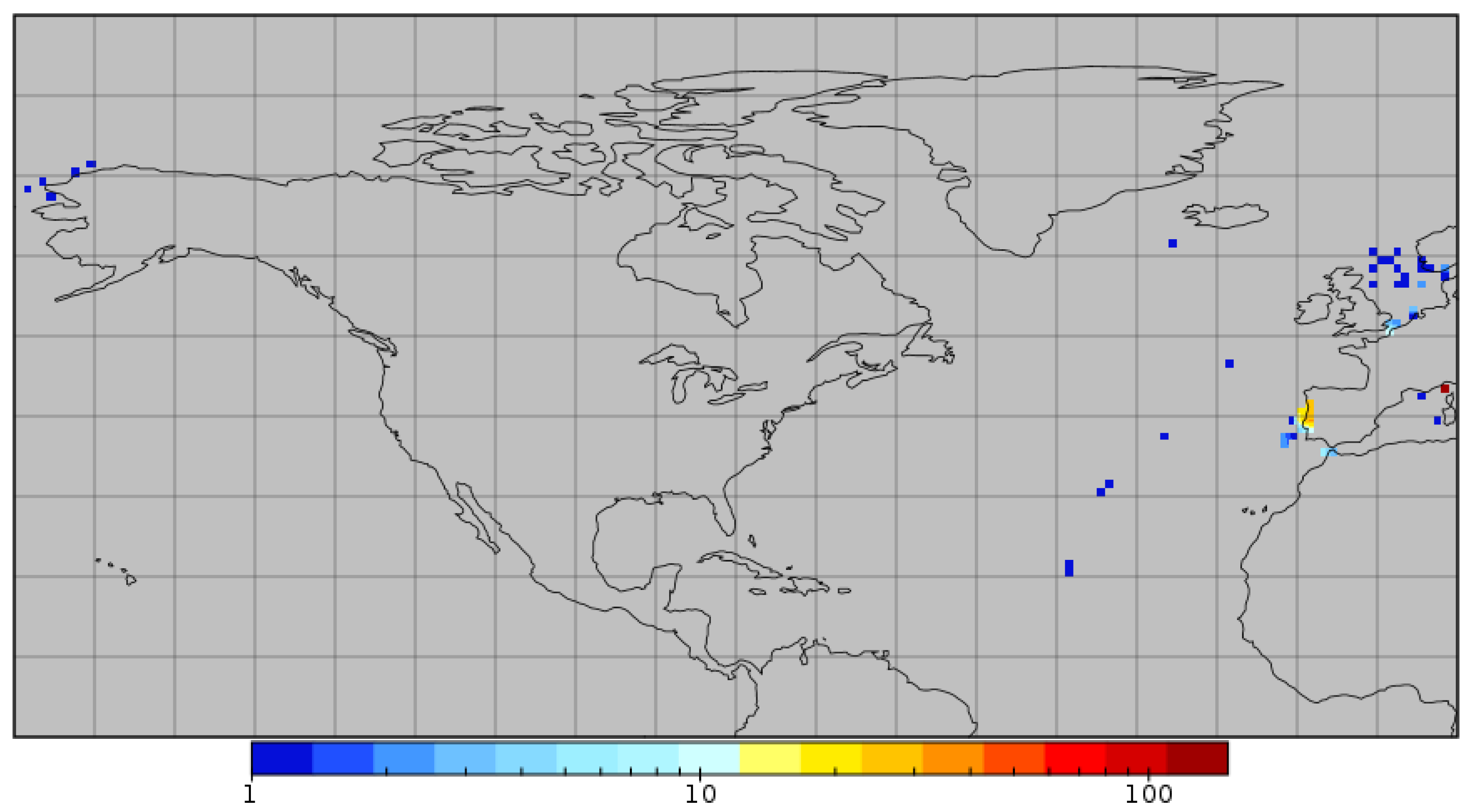
2.1. Data—The Matchups Database

The starting point for this work was a dataset of 359 in situ High Performance Liquid Chromatography (HPLC) surface ocean chlorophyll-a (chl) measurements from 2002 to 2011, mostly from European shelf seas but including some data from the open North Atlantic, the Mediterranean, and the North Pacific (Figure 1). We created a database of matchups between these in situ data and chl estimates from NASA’s MODerate resolution Imaging Spectrometer sensor on the Aqua satellite (MODIS-Aqua), V2012.0 reprocessing [12] using the standard OC3 chl algorithm [13]. Henceforth, we will refer to in situ chl as chl_IS and satellite observed chl as chl_SAT.

For each chl_IS measurement, we searched for all overlapping MODIS-Aqua overpasses within ±12 h. This is a larger range than normally used for matchups, allowing us to investigate the effect of time difference on matchup uncertainty. For each overlapping overpass, we formed a 3 × 3 pixel grid of the nearest pixels to the in situ measurement, treating each pixel as an independent matchup. Note that due to the unusual geometry of the MODIS-Aqua sensor [14], these may not be from adjacent MODIS-Aqua scan lines. This gave a total of 2951 satellite-in situ comparisons (matchups), consisting of up to nine satellite pixels for each in situ measurement. Each pixel was stored as a separate line of the matchups database, recording the in situ date, time, latitude, longitude, and chl_IS, and the satellite granule ID, time difference, chl_SAT, sun and view zenith angles, wind speed, glint radiance at 869 nm, aerosol optical depth at 869 nm, R_rs in all visible and near infrared bands (see

Table A1. Explanatory variables investigated with gamlssCV, functional forms in the mean and SD models, order of addition (1 = first) and SD_PRED. Variables with blank lines were not chosen by gamlssCV.

Variable	Functional form in Mean Model	Order of Addition to Mean Model	SDpred	Functional form in SD Model
ln(chlSAT)	pb	1	0.79
Day of year	pbc	4	0.28
Day length	ps	2	0.32
Satellite age	ps	5	0.14
1/cos(solar zenith angle)
1/cos(view zenith angle)	ps	10	0.30
Airmass	ps	9	0.27
Wind speed
Aerosol optical depth at 869 nm
Glint radiance at 869 nm
Rrs(412)	ps	3	0.78
Rrs(443)
Rrs(469)	ps	6	1.21
Rrs(488)
Rrs(531)	ps	7	0.65
Rrs(547)	ps	11	0.76
Rrs(555)	ps	12	0.66
Rrs(645)				ps
Rrs(667)
Rrs(678)
Time difference	ps	8	0.11

), and all Level 2 flags.

Note that the satellite data corresponding to each in situ measurement are spatially very close and so are very unlikely to be independent, but we did not expect this to be a serious problem for the statistics, since our aim is to predict the response variable as a function of the explanatory variables rather than to establish causative relationships. We also considered that the differences between satellite pixels compared to the same in situ measurement could give us insight into the sources of uncertainty in the satellite measurement. Reducing to 359 matchups, e.g., by choosing only the closest valid satellite pixel, would not have allowed us to demonstrate the potential of the method. See Section 2.3 and Section 3.1 for unexpected consequences of this decision.

2.2. Candidate Explanatory Variables

We considered the following variables as candidates to explain satellite chl errors (see Table A1 for a full list of variables investigated in GAMLSS):

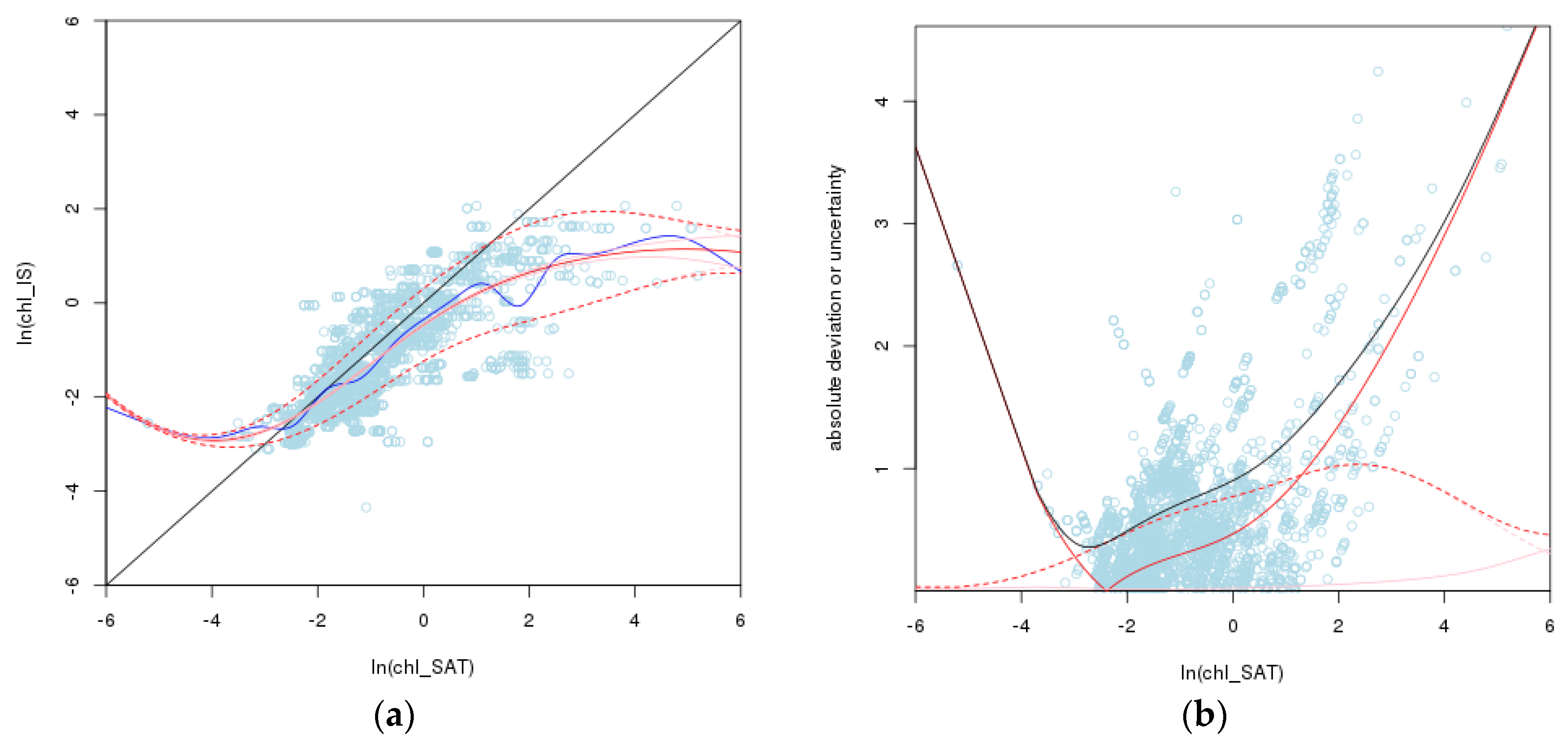
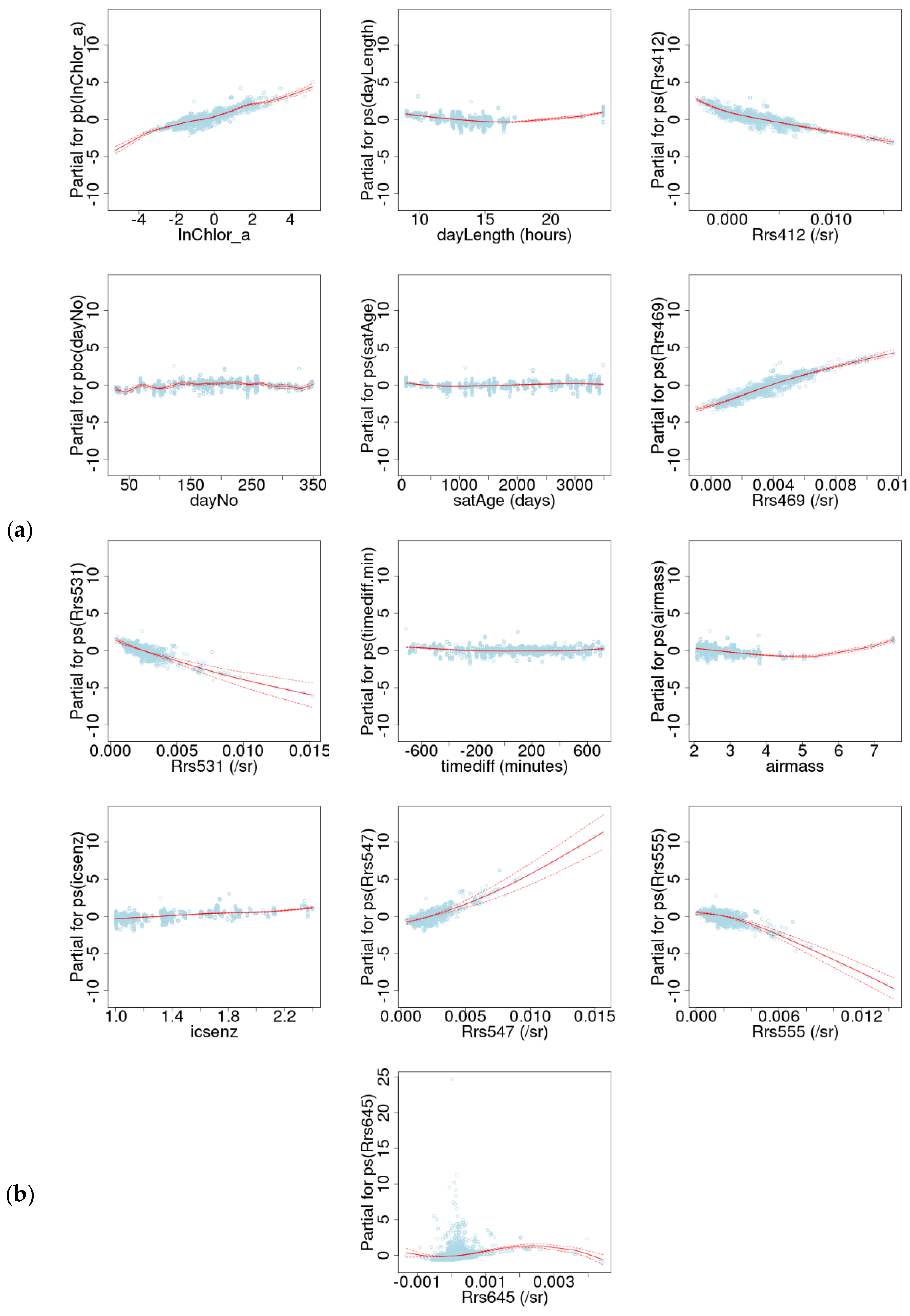
• We expect chl_SAT itself to be related to chl errors. The first indication that the chl retrieval has failed is usually the presence of outliers, or implausible values of chl_SAT. Also, the task of retrieving chl in oligotrophic waters is very different from that in highly eutrophic waters, so we expect retrieval uncertainty to vary with chl [15]. We therefore included ln(chl_SAT) as a candidate explanatory variable. Other derived geophysical products that could give insight into the performance of the chl algorithm, such as inherent optical properties, could also be used.
• The standard OC3 MODIS-Aqua chl algorithm is based on ratios of R_rs [13], so we expect R_rs at different wavelengths to affect errors in different ways. The R_rs spectrum is also indicative of water type [6], with different water types having different effects on atmospheric correction (e.g., highly scattering waters are bright in the near infrared) and on the quality of chl retrievals (e.g., highly absorbing waters can give erroneously high chl values) [15]. Here, we represented the R_rs spectrum by simply including all visible wavelength spectral bands of R_rs, though many other combinations such as R_rs ratios may also be useful. See Table A1 for a list of spectral bands used.
• The solar and view zenith angles affect retrievals through atmospheric and surface effects. When light passes obliquely through the atmosphere, it is attenuated more than a vertical beam, and it also becomes harder to predict the effect of interaction of the light with the atmosphere and the sea surface; hence, atmospheric correction uncertainty is expected to increase [16]. The solar zenith angle also affects the amount of light available to phytoplankton at the time of measurement. We represented solar and view zenith angles with 1/cos(zenith angle), a measure of how much atmosphere light has to pass through without being absorbed or scattered. We also represented the airmass as 1/cos(solar zenith angle) + 1/cos(view zenith angle), a measure of the total atmospheric path length from sun to satellite via the sea surface.
• Wind speed affects retrievals through disturbance of the sea surface, making it more difficult to predict its effect on incident light, particularly at high zenith angles [17]. Wind can also create wave breaking and surface foam, which appears bright in the near infrared, potentially causing problems for atmospheric correction [18].
• Sun glint is bright in the near infrared and can cause problems for atmospheric correction. It can be modeled as a function of wind speed, view geometry, and wavelength [17], and we would like to represent sun glint with the modeled glint at 869 nm. However, in the matchups database there were many pixels for which this product was missing, and we could find no satisfactory way of including an explanatory variable with so much missing data, so this variable was excluded from analysis.
• Aerosol haze makes retrieval of chl more difficult by scattering and absorbing light [19]. Thin or sub-pixel cloud that does not trigger the CLDICE flag is also interpreted as aerosol in MODIS-Aqua processing [20]. We would like to represent aerosol with the retrieved aerosol optical depth at 869 nm, but again there were many pixels for which this product was missing, so it was excluded. Although sun glint and aerosol are not used in this analysis, they are mentioned because they are likely to be important sources of uncertainty in satellite ocean colour.
• The date could influence chl uncertainty in two ways, through long-term changes and through seasonal variations. Long-term changes could be due to sensor degradation with time [21], or to climatological ecosystem changes, which could affect the quality of chl retrievals from space. We represented long-term changes with the satellite age in days to try to detect sensor degradation effects, since here we are only dealing with one satellite. If multiple sensors were used, we could try to distinguish changes due to sensor degradation from those due to ecosystem changes by looking for sensor-specific changes. Seasonal variations could be due to the seasonal cycle of phytoplankton, or to optical changes, the most obvious of which is the change in sun zenith angle. We represented this with the day of year, which should be represented as a cyclic function with a 365-day cycle. Our data are all in the northern hemisphere, but if data from both hemispheres are used, it may be necessary to create an interaction term between latitude and day of year.
• Latitude (together with day of year) determines the day length, a fundamental influence on phytoplankton ecology, as well as the solar zenith angle. Ocean circulation patterns also tend to segregate the oceans into zonal provinces (e.g., [22]). Our in situ data are geographically too sparse to reliably distinguish provinces, so instead of using latitude directly, we used day length calculated from latitude and day of year, as well as solar zenith angle (see above).
• The time difference between satellite and in situ measurements obviously has a potential impact on the quality of the retrieval, and this is traditionally accounted for by imposing a maximum time difference on matchups, e.g., ±6 h. This approach has the same drawback as the Level 2 flags: that a measurement slightly less than 6 h away from the in situ measurement, that almost exceeds several other mask thresholds, is given full weight in calibration or validation exercises, while one slightly more than 6 h away that is otherwise exemplary is given zero weight. We included time difference as an explanatory variable in order to try to quantify its effect. This might shed light on the choice of maximum time difference, as well as allowing us to weigh calibration or validation measurements according to time differences. We would actually expect this uncertainty to be dependent on how rapidly chl is changing at the point of measurement. Given sufficient data, it may be possible to distinguish different weightings or maximum time differences in different regions. Another possible way that time differences could influence retrieval quality is through diurnal changes in chl. Since a sun-synchronous satellite measures at approximately the same time of day everywhere, this effect would be seen as a bias due to time difference for a given satellite orbit, while we might expect differences due to non-diurnal changes to occur as often in one direction as the other, and so appear as an increase in SD.
• Level 2 flags are intended to inform users of the circumstances surrounding the pixel measurement. Some are simply informative (e.g., this is a land or shallow water pixel), some are warnings (e.g., suspected sun glint), and some denote errors (e.g., atmospheric correction or chl algorithm failure). The aim of this work is to replace flag-based approaches with continuously varying uncertainties, so we did not include Level 2 flags. However, we did examine the effectiveness of level 3 masking in eliminating pixels with large errors, and the results were not as expected. Histograms of δln(chl) = ln(chl_SAT) − ln(chl_IS) for both the whole dataset and only pixels masked at level 3 showed that the pixels masked at level 3 had a consistently lower bias, with a root mean squared δln(chl) of 0.871 for the whole dataset and 0.714 for the pixels masked (i.e., rejected as suspected low quality) at level 3. This is the opposite of the intended effect of masking.
• Chlorophyll can exhibit high variability on many spatiotemporal scales, and we would expect high variability on the scale of the satellite-in situ comparison (up to a few km and hours) or smaller to result in increased chl discrepancies. We represented spatial variability with the SD of the ln(chl_SAT) associated with each chl_IS, of which there can be up to nine. This combines two possible effects, spatial variability in chl, and effects causing changes in chl_SAT such as stray light. MODIS-Aqua data generally recur in a given location once a day at best except at high latitudes, so representation of temporal variability is not possible using these data. HPLC is time consuming and expensive, so in situ HPLC data with high spatiotemporal resolution are rare. However, if this analysis were repeated using in situ data with the appropriate resolution, such as fluorometric chl from autonomous sensors, the effect of in situ chl variability could be studied.
• The number of valid chl values in the 3 × 3 grid, either at level 2 or 3, is an indication of the presence or absence of features such as clouds or land that may increase uncertainty in the remaining values. Here, we used the number of valid chl values at level 2.
• If a more analytic uncertainty model is available, then the outputs of this (e.g., bias and SD, or just overall uncertainty) may be used as inputs to this model. If the prior model is perfectly successful, then, e.g., output bias will equal input bias with no other dependencies. It is far more likely that other dependencies exist, giving insight into how the prior model can be improved.

There are many other plausible explanatory variables than those described above, and the most challenging part of applying this method is to find the set of explanatory variables that best describes the behaviour of the response variable. This set is the best we have found so far for this dataset, and serves to illustrate the concept.

2.3. Statistical Modeling

In this work we take our measure of chl_SAT uncertainty to be δln(chl), which we assume to be normally distributed, neglecting chl_IS uncertainties [23]. Initial work focused on [δln(chl)]² as a measure of the overall uncertainty, but this loses the distinction between bias and SD, and between positive and negative bias. Plotting δln(chl) or ln(chl_IS) as a function of ln(chl_SAT) shows the expected clear positive bias at high chl_SAT and a slight negative bias at low chl_SAT (Figure 2a, small circles and solid grey 1:1 line). Applying a traditional simple error analysis with globally constant bias and SD, δln(chl) has mean (bias) 0.37 and SD 0.79, with a root mean square deviation (RMSD = $\sqrt{\overline{\mathsf{\delta }\ln {\left(\mathrm{chl}\right)}^2}}$) of 0.87 in natural log space. Simple subtraction of the global bias would reduce the RMSD to 0.79, explaining 18% of the squared deviation, though it is clear from Figure 2a that significant biases would remain in the data, and this may increase bias at intermediate chl values.

The GAMLSS tools gamlss and gamlssCV represent this as a model (mean or SD) containing only a constant term, which is adjusted to minimise the global deviance. The mean deviance for this model found by gamlss is 2.362, and that found by gamlssCV is 2.377; the small difference (0.016) shows, as expected, that this model is not significantly over-fitted.

As an illustration of the use of the GAMLSS package, we will explore a simple model of δln(chl) as a function of ln(chl_SAT) (see

Table A2. Models of δln(chl) as a function of ln(chl_SAT), their mean deviance using gamlss and gamlssCV, and the percentage of squared deviation explained by the mean model.

Model or Change from Previous Model	Mean Deviance (Improvement over Previous Best Model)		gamlssCV-Gamlss	RMSD	Percentage of Squared Deviation Explained
	Gamlss	GamlssCV
Original data	-	-	-	0.87	-
Constant mean and SD	2.362	2.377	0.016	0.79	17%
Linear mean	2.095(0.266)	2.121(0.256)	0.025	0.70	37%
ps mean	2.027(0.068)	2.077(0.044)	0.05	0.682	39%
pb mean	1.964(0.063)	2.065(0.012)	0.101	0.68	40%
ps SD	1.841(0.123)	1.993(0.072)	0.152	0.68	40%

for detailed results). When we replace the basic model above with the simple but implausible choice of a linear mean model, i.e., modeling the mean of δln(chl) as a linear function of ln(chl_SAT) with a constant SD, the mean deviance reduces by 0.266 with gamlss and 0.256 with gamlssCV, and the difference between the two increases to 0.025. Using the GAMLSS ps (cubic spline) function for the mean but still with a constant SD, the mean deviance is reduced by 0.068 with gamlss and 0.044 with gamlssCV, and the difference increases to 0.05. This model is shown in Figure 2a as a solid red line. If we replace the ps function with the more responsive pb (beta spline) function, shown in Figure 2a as a solid blue line, the mean deviance is reduced by 0.063 with gamlss and 0.012 with gamlssCV, with a difference of 0.101. In this example, the pb function is not over-fitted in comparison to ps, but the improvement in mean deviance (0.012) is much less than that suggested by gamlss (0.063).

The GAMLSS package is also able to model the SD (actually ln(SD) to give it an infinite range) as a function of the explanatory variables. For instance, adding a model of ln(SD) as ps(ln(chl_SAT)) to the ps mean model reduced the mean deviance by 0.123 with gamlss and 0.072 with gamlssCV, with a difference of 0.152. The increasing difference from simple to more complex models highlights the increased need for independent checking as the model complexity increases, but the gamlssCV mean deviance of the final model is the lowest found so far (by 0.017), so the new model is not over-fitted in comparison to the previous models. The final model has a RMSD of 0.68, explaining 40% of the deviation as bias. By investigating changes to the best model and choosing those changes that decrease the gamlssCV mean (or global) deviance most, we optimise our model.

The gamlss tool also estimates the standard error (SE, an estimate of the uncertainty of the mean model) as a function of the explanatory variables, so we have bias, SD, and SE as three separate measures of the uncertainty in ln(chl_SAT). Note that SE as used here is not the same as the SE of a dataset, commonly evaluated as SD/$\sqrt{N}$. To evaluate the overall uncertainty, we use the square root of the sum of the squares of bias, SD, and SE (the root squared sum, henceforth RSS), i.e., we assume them to be uncorrelated. A more rigorous treatment would account for covariance between them, which could be calculated from the training data, but this approximation is sufficient to illustrate the method. This uncertainty can be evaluated for any combination of explanatory variables, allowing us to produce uncertainty maps for arbitrary satellite data. If the mean is subtracted from ln(chl_SAT) to give a bias-corrected estimate of ln(chl_IS), the remaining uncertainty is the RSS of SD and SE.

Figure 2a shows the results of this process for ps models of the mean and SD of δln(chl), with the pb model of the mean shown in blue for comparison, and Figure 2b shows the contributions to uncertainty. Figure 2 shows a curious effect, that SD reduces towards zero at the extremes of the distribution, most markedly at low δln(chl). On investigation, it was found that the point in Figure 2 with the lowest δln(chl) is actually two points from the same matchup (hence with the same ln(chl_IS)) that also both have the same ln(chl_SAT). This can happen because the satellite product is stored digitally, so two pixels with the same digital number will be ascribed exactly the same chl value. The calculation of the mean is robust with respect to such duplication, but the calculation of SD is not. In the absence of other points nearby, the presence of two identical values implies a local SD of zero, forcing a responsive model of SD towards zero. When these points are at the tail of the distribution, as in this case, the result is that the model SD tends strongly towards zero as the tail is approached.

Next, we used the GAMLSS package to find more complex models with a better fit to the data. First, we scaled all potential explanatory variables in the matchups database to have a mean of 0 and a SD of 1, keeping a record of the original mean and SD. We then applied the methodology of stepGAIC to gamlssCV to find the combination of explanatory variables that minimised the cross-validated global deviance. This methodology is as follows [9]:

• Start with a basic model (we used constant mean and SD);
• Try adding each explanatory variable in turn to the mean and keep only the one with the lowest global deviance;
• Repeat 2, adding further variables to the mean until no variable improves the global deviance;
• Repeat 2–3, adding variables to the SD;
• Try removing each variable in turn from the SD and keep only the removal that results in the lowest global deviance. Repeat until no variable removal improves the global deviance;
• Repeat 5, removing variables from the mean.

For each variable, we tried both the pb and ps functions (only pbc in the case of the day number), each with a number of degrees of freedom derived from the data [9]. In steps 5 and 6, we tried replacing pb with ps or vice versa, as well as removing the variable entirely.

2.4. Application to Satellite Data

The aim of this example was not to create a model to describe the behaviour of in situ-satellite matchups, but to present a method for quantifying the uncertainty in arbitrary satellite data. Hence, the model needed to be further developed to allow this to happen. At each pixel of a satellite overpass, all the explanatory variables used in the model (with the exception of the time difference, which we set to zero) are available, either from the satellite measurements or from ancillary data such as wind speed. After normalising each variable using its mean and SD from the training data, the predict function from the GAMLSS package can be used to create maps of model predicted bias, SD, and SE of ln(chl) at each pixel. In GAMLSS 5.0.0, the predict function can only predict SE for the training data, not for new data, so we linearly interpolated and extrapolated ln(SE) from the training data to the new data for each explanatory variable, then estimated the overall SE as the RSS of its components.

In principle, the bias can be subtracted from the satellite retrieval to give an improved estimate of chl_IS, but it is possible that information is lost or distorted in this process. For example, if the spatial noise in the bias image is greater than its magnitude, bias subtraction will result in increased noise without meaningful improvement and could potentially obscure features visible in the uncorrected image.

Explanatory variables that are crude representations of the actual errors may also add artefacts. For instance, the representation of errors as a function of latitude or day length could introduce zonal striping to the bias-corrected image, or the use of low radiometric resolution bands to characterise bias could lead to a bias-corrected image with degraded radiometric resolution. Hence, we recommend that, where possible, bias-corrected images should be used in conjunction with the uncorrected images (the former to remove artefacts due to bias and the latter to visualise or analyse features that are not affected by bias). If a feature in the original image is weaker or not present in the bias-corrected image, the feature is likely to be due to bias. Conversely, if a feature is present in the corrected image but absent in the original image, the feature may be due to model artefacts. This problem can be mitigated by careful choice of explanatory variables, e.g., if chl errors are a function of latitude, but the main underlying reason is changes in solar zenith angle, a model using solar zenith angle is less likely to produce artefacts than one using latitude.

When creating composites (e.g., monthly) of overlapping satellite overpasses, overpass pixels contributing to a given composite pixel may be weighted according to their model uncertainties. As with each overpass, this could be done with the original chl_SAT with uncertainty equal to the combined bias, SD, and SE, or with bias corrected chl_SAT with uncertainty equal to combined SD and SE. If the uncertainty model is sufficiently accurate and comprehensive, this should result in a reduced incidence of outliers in composites, as well as giving per-pixel composite uncertainties and reducing, or perhaps even eliminating, the need for masking of suspect data.

3. Results

3.1. Model Dependencies

The best model found for the mean in steps 2–3 (Section 2.3), with terms listed in order of addition, was pb(ln(chl_SAT)) + ps(day length) + ps(R_rs(412)) + pbc(day of year) + ps(satellite age) + ps(R_rs(469)) + ps(R_rs(531)) + ps(time difference) + ps(airmass) + ps(1/cos(view zenith angle)) + ps(R_rs(547)) + ps(R_rs(555)). The best model found for the SD in step 4 consisted only of ps(R_rs(645)), noting that the failures of the gamlss function referred to in Section 2.3 mean that this is probably not an optimal SD model. It also exhibits the problem described in Section 2.3, that the SD tends to zero at extreme values, in this case high values. There were no changes made in steps 5–6. The apparent mean deviance using gamlss was 0.98, accounting for 76% of the squared deviation as bias, and the actual mean deviance using gamlssCV was 1.49, accounting for 67% of the squared deviation as bias. This model performs significantly better than the best model found using ln(chl_SAT) alone (mean deviances 1.84 and 1.99, actual squared deviation explained 40%).

The final model dependencies are shown in Figure 3. The SD of the model predictions at the matchup points (SD_PRED) is used as a measure of the magnitude of the impact of the explanatory variable on the bias, and is shown in Table A1. Care should be taken to distinguish SD_PRED from the model prediction of the SD of δln(chl), and to distinguish the order of these impact values from the order in which variables were added to the model, which is a measure of the impact of inclusion of the variable on the model’s ability to represent the residual (defined as (measured value − mean)/SD) as normally distributed with mean 0 and SD 1. This is not the same as the model explaining the variance of the data, for example, and selection of a new explanatory variable can change the impact of the previously selected variables, so there is no guarantee that the impacts will decrease with order of selection.

The mean (bias) in the final model is determined primarily by R_rs(469) (SD_PRED = 1.21), with lesser effects from ln(chl_SAT) (0.79), R_rs(412) (0.78), R_rs(547) (0.76), R_rs(555) (0.66), and R_rs(531) (0.65), and much lesser effects from day length (0.32), 1/cos(view zenith angle) (0.30), day of year (0.28), airmass (0.27), satellite age (0.14), and time difference (0.11). The explanations for these explanatory variables can be found in Table A1. It is interesting that R_rs(547) and R_rs(555) were the last to be selected but have among the highest impact on the bias, and that the two wavelengths are very close together but have opposite impacts, suggesting that the ratio of the two is an important factor in determining satellite chl bias. R_rs(547) is an important part of the MODIS-Aqua OC3 chl algorithm, forming the denominator of the band ratios used to calculate chl, but R_rs(555) is not used in the OC3 algorithm, because it has lower sensitivity than R_rs(547).

With this dataset, we found that when trying to add variables to the SD in step 4, the call to the gamlss function would frequently fail for certain gamlssCV subsets while returning the best global deviance for others, excluding the model from further analysis but implying that the candidate model would have been the best so far had the failure not happened. We suspect that this is due to the presence of the duplicate values mentioned in Section 2.3, as it does not occur for other similar datasets without such duplicates.

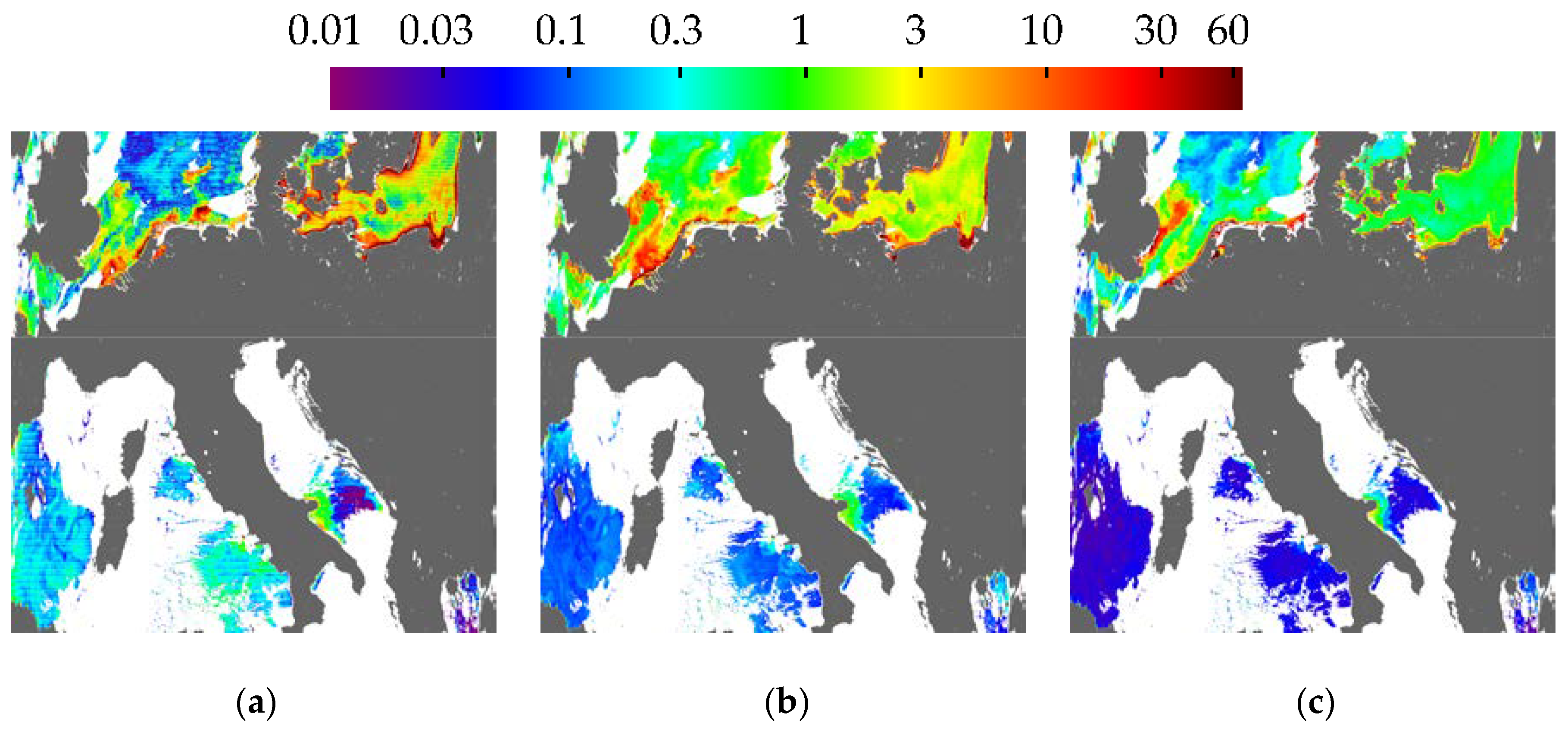
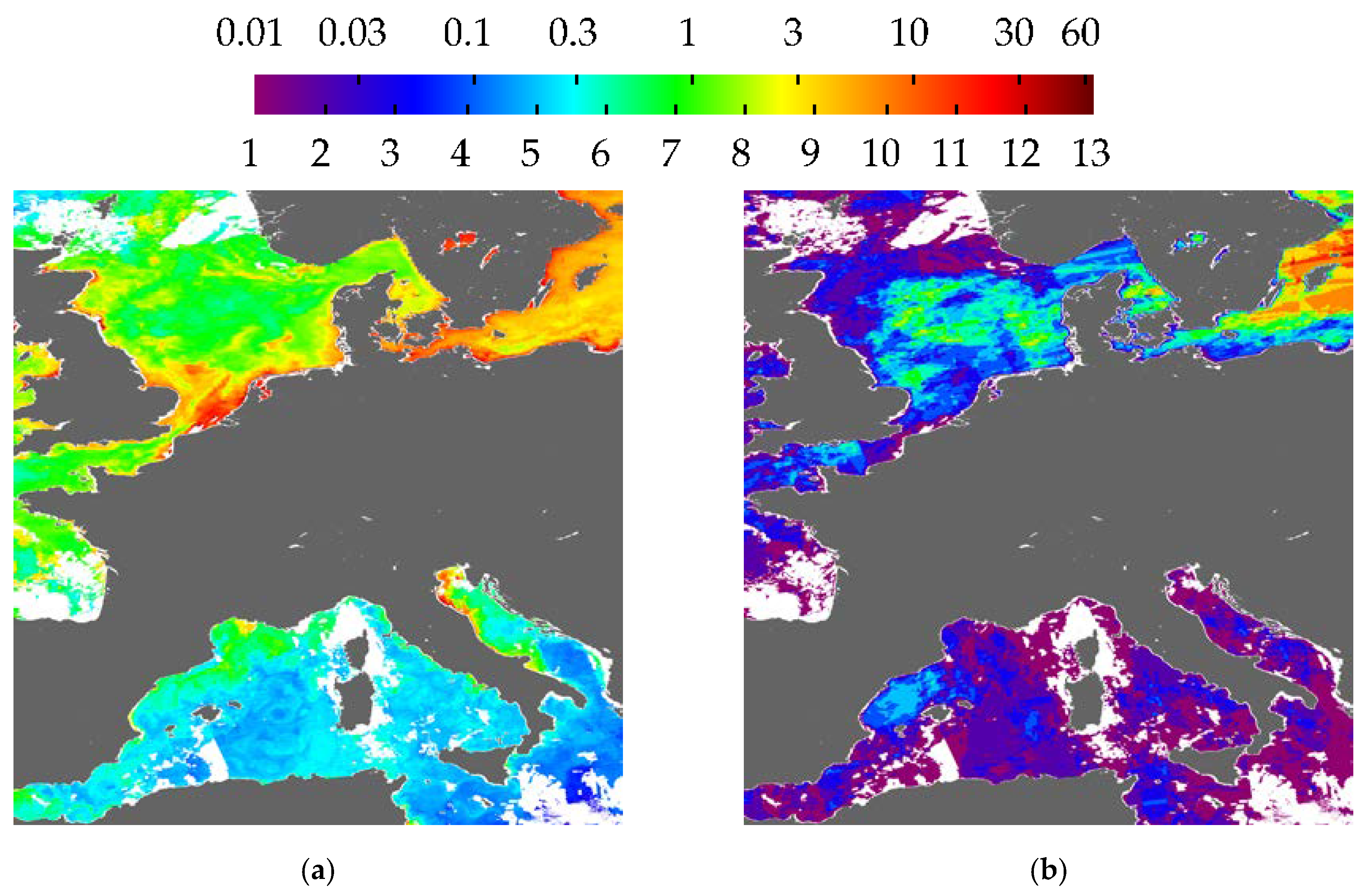
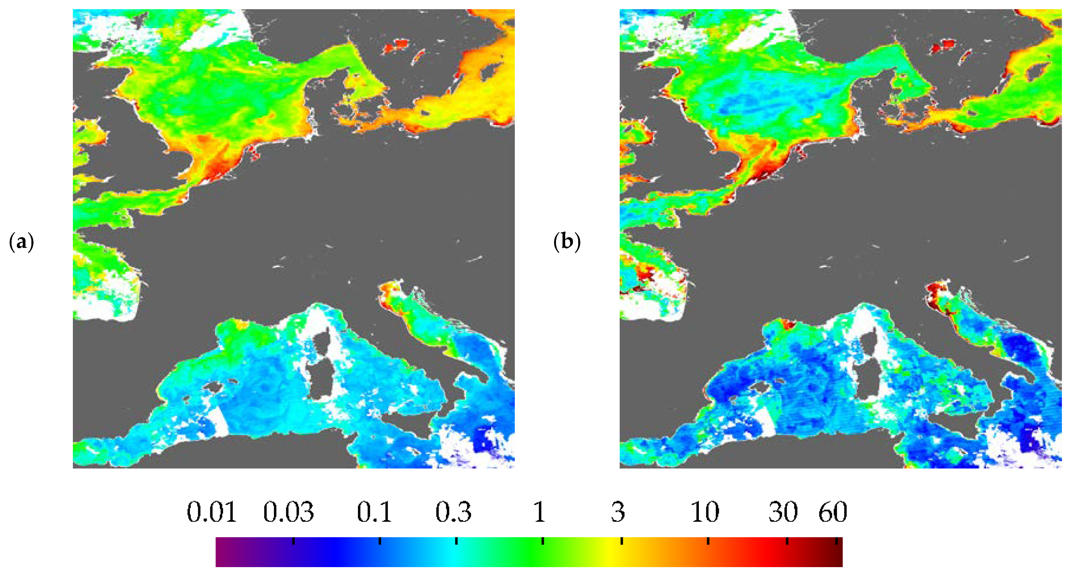
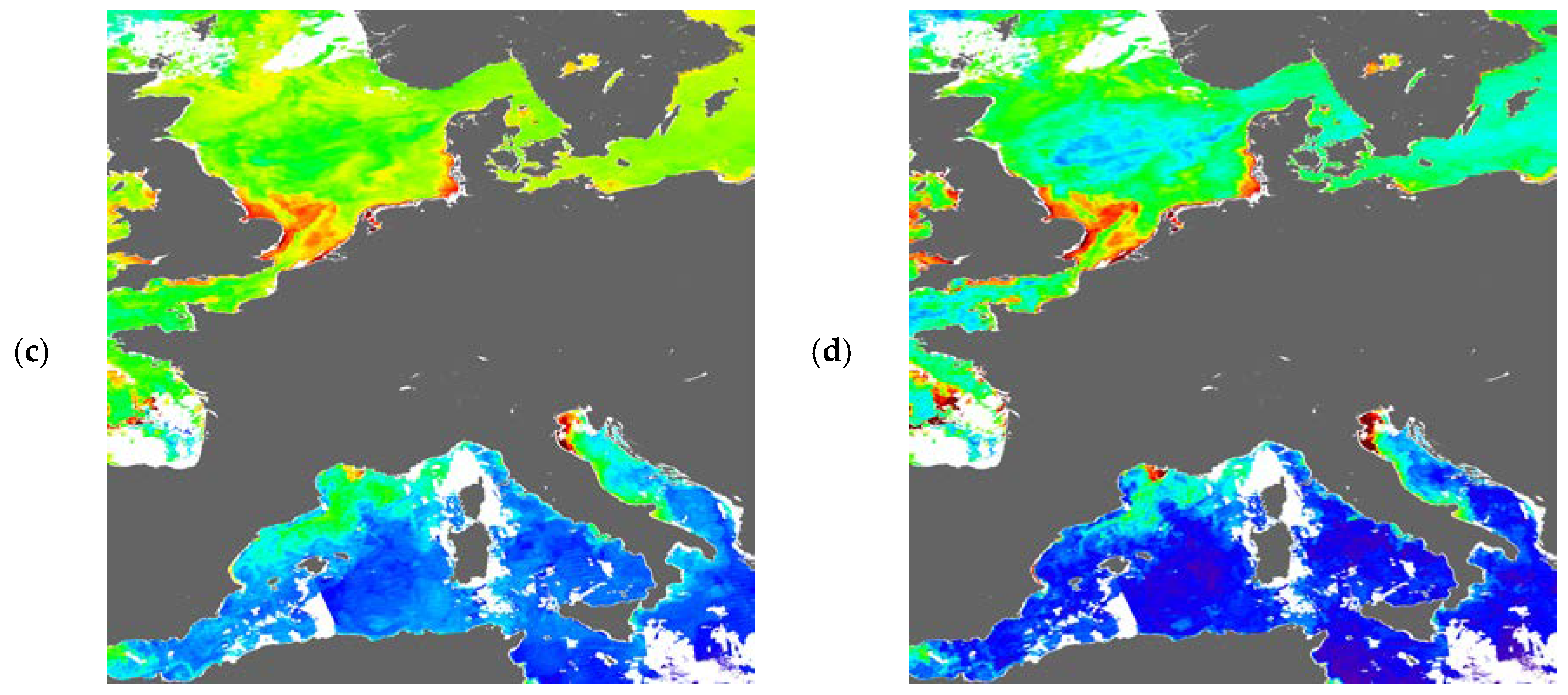
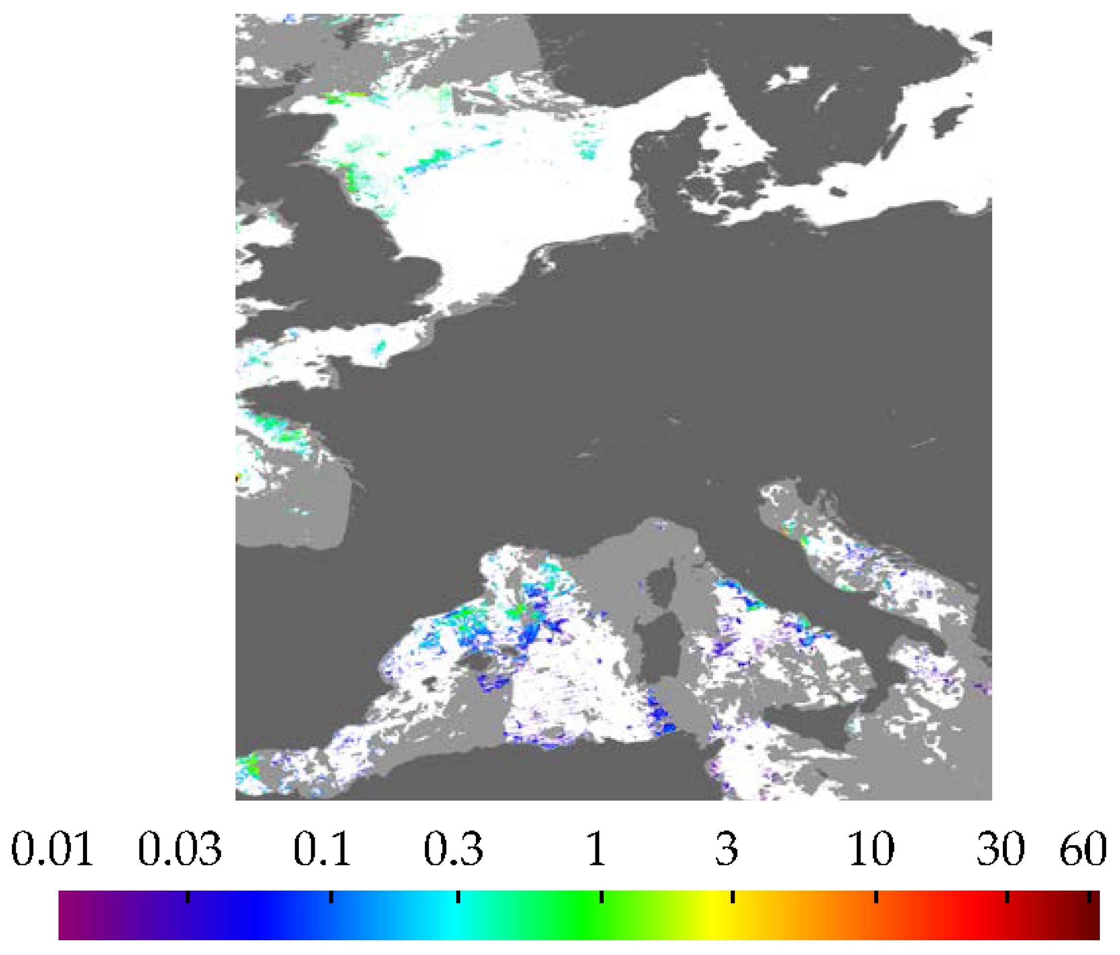
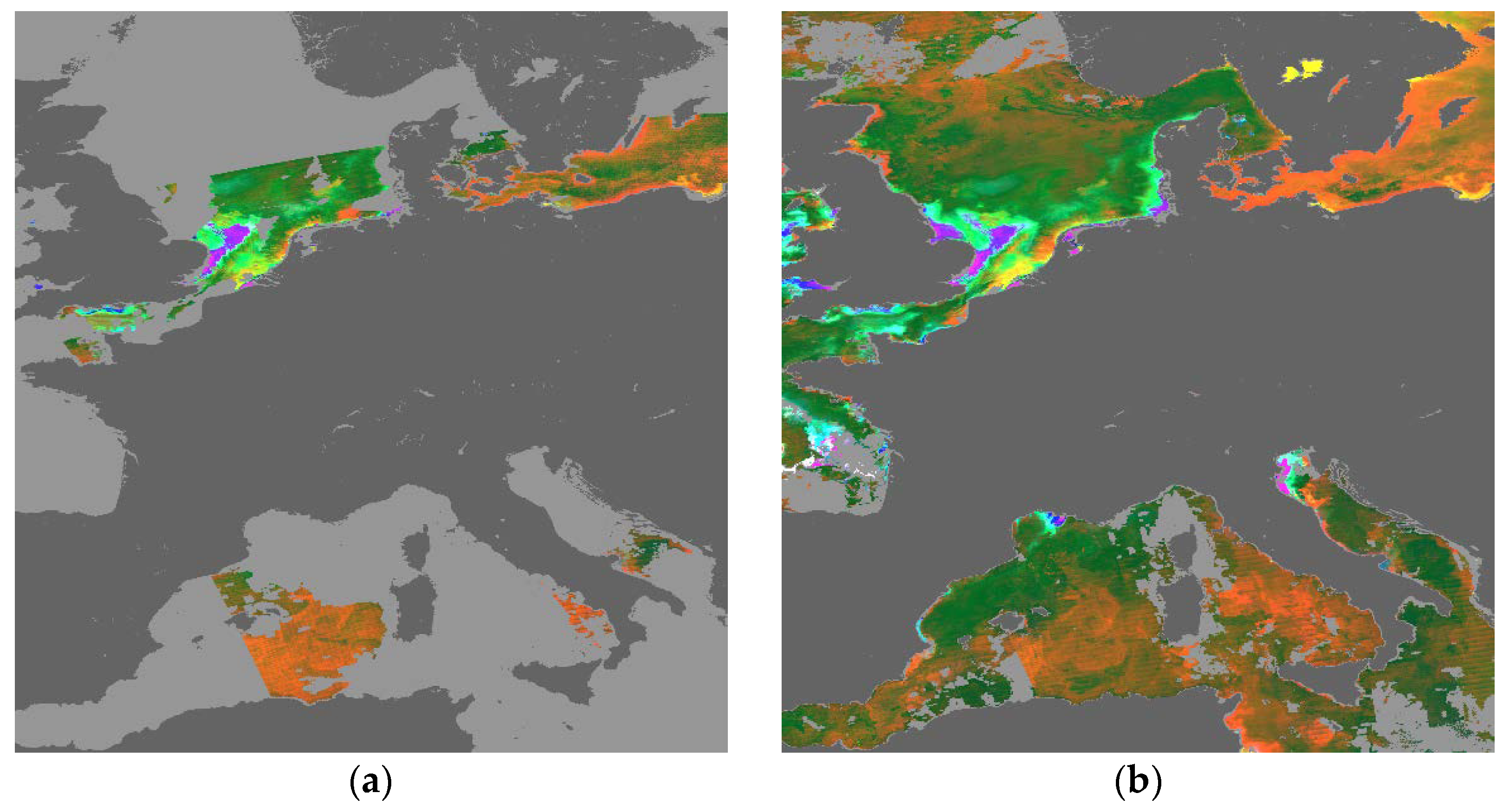
3.2. Visualisation of Uncertainties

Armed with the best model we could find to account for the differences in ln(chl) in the matchups dataset, we then used this model to produce chl uncertainty maps for some sample MODIS-Aqua data. Since most of our matchups occurred in European waters, we chose a relatively clear MODIS-Aqua scene covering the North Sea and western Mediterranean, on 5 May 2013 at 12:10 (Figure 4a), processed using version 7.0.2 of the SeaDAS processing package [24]. This is the version corresponding to the MODIS-Aqua V2012.0 reprocessing used for the matchups database [12].

We used the predict function from the GAMLSS package together with the explanatory variables taken from the MODIS data to calculate the mean, SD, and SE of δln(chl), shown in Figure 5a–c and Figure A1. To prevent SD tending to zero for very large values of R_rs(645) (see Figure 3b), SD values lower than those found by applying the SD model to the training data are set to the minimum of these values. To convert these to an estimate of overall uncertainty in chl, we multiplied their RSS by chl_SAT (Figure 4b). Comparison of Figure 4a,b shows high uncertainty in coastal zones, river plumes, and the Baltic Sea, all areas where satellite chl algorithms are known to have problems, especially where chl_SAT is implausibly high, so this initial uncertainty map looks plausible and has no obvious model artefacts such as banding or noise.

Next, we subtracted the bias from ln(chl), shown in Figure 4c, and calculated the bias-corrected uncertainty as the RSS of SD and SE, shown multiplied by chl_SAT in Figure 4d. The distribution of chl shown in Figure 4c looks much more plausible than that in Figure 4a, and areas where it remains implausibly high, e.g., North Sea river plumes and the Baltic, have correspondingly high residual uncertainty in Figure 4d.

3.3. Effect on Composites

We chose a region from 35 to 61°N, 5°W to 20°E, encompassing the North Sea, the western Mediterranean, and parts of the Baltic Sea and the Bay of Biscay in a simple 0.01° (1.1 km North-South) nearest-neighbour geographic projection, and formed an 8-day composite from 48 MODIS-Aqua overpasses from 1 to 8 May 2013 processed as described above, applying Level 3 masks as in the standard NASA compositing approach and taking the mean of ln(chl) where a composite pixel was formed from multiple overpasses. The resulting composite is shown in Figure 6a, and the number of passes used to create the mean at each pixel is shown in Figure 6b.

We then mapped the bias, SD, and SE of ln(chl) for each overpass to the same grid, and used them to generate weighted composites. We formed uncorrected and bias corrected composites using a weighted mean with weight equal to uncertainty⁻². It would also be desirable to generate maps of the composite uncertainty and produce combined maps similar to those in Figure 4. If only one overpass contributes to a map grid cell, the uncertainty is the same as in Figure 4. With more than one overpass, simple error propagation assuming uncorrelated errors gives us a composite uncertainty equal to $\sqrt{\sum {\left(w\sigma \right)}^2}/\sum w$, in which w is the weight of each overpass in the grid cell and σ is its uncertainty. Applying w = σ⁻² gives composite uncertainty equal to $1/\sqrt{\sum w}$. Note, however, that uncertainties are very likely to be correlated in this case.

If we assume that all overpasses at a given grid cell are samples of a constant underlying ln(chl) equal to μ_c, the uncertainty model predicts that each bias-corrected ln(chl) measurement would be distributed with measurement-independent mean μ_c and a measurement-dependent standard deviation σ_c equal to $\sqrt{{\mathrm{SD}}^2+{\mathrm{SE}}^2}$, assuming uncorrelated errors. If we assume μ_c to equal the bias-corrected weighted mean calculated above, we can subtract this from all measurements and divide each measurement by its σ_c to give a ‘model residual’, which should be distributed with mean 0 and standard deviation 1. However, there may also be natural variation in ln(chl) between measurements, a further source of composite uncertainty not included in the model.

For composite grid cells with more than one pass, we can calculate the actual sample standard deviation σ_r of [ln(chl) − bias − weighted mean]/σ_c and, if this is greater than 1, attribute the excess to natural variation in ln(chl) between measurements with a standard deviation of σ_n. Assuming all terms to be uncorrelated, ${\sigma }_c^2$ then becomes ${\mathrm{SD}}^2+{\mathrm{SE}}^2+{\sigma }_n^2$. At each grid cell with σ_r greater than 1, we assume that σ_n is constant across overpasses, i.e., we allow it to vary spatially across the image but not temporally over the time range of the composite. We used Newton-Raphson root finding to estimate σ_n, at each iteration recalculating the weighted mean and all σ_c until σ_r converges to 1. The resulting uncorrected composite is shown in Figure 7a and its uncertainty $\sqrt{{\mathrm{bias}}^2+{\sigma }_c^2}$ in Figure 7b. The bias-corrected composite is shown in Figure 7c, with uncertainty σ_c shown in Figure 7d. σ_n is shown in Figure 8.

Comparison of Figure 6a and Figure 7a shows little change due to weighting for the unmasked pixels, suggesting that unmasked uncertainties are dominated by geographical location rather than variation between passes in a given grid cell. An exception is the southern Baltic, where the number of passes per grid cell is highest, uncertainties are large, and weighted chl appears to be more realistic than unweighted [25].

Inspection of Figure 7 shows that the anomalously high chl in the Baltic and the Swedish great lakes becomes comparable to that in the open North Sea after bias correction, while chl in the open Mediterranean is reduced to values typical of the oligotrophic eastern basin (southeast of Italy and Sicily), though it is unclear whether the low values in the western basin are more or less realistic than the uncorrected values. The uncertainty maps appear to successfully highlight regions of implausibly high chl such as North Sea river plumes.

Figure 8 shows that it is rarely necessary to invoke natural variation to explain the variability between passes. This suggests that the model is overestimating uncertainty in this case, since even with no natural variation we expect the sample standard deviation to exceed that of the underlying distribution about 50% of the time. This is despite the assumption of uncorrelated errors, which causes overall uncertainty to be underestimated if correlations are positive. This observation could, in principle, be used to adjust model uncertainties to be consistent with the observed variations.

4. Discussion

The above results, though they appear very promising, should be seen as preliminary. The matchups database has sparse spatial coverage, and improvements in MODIS-Aqua processing since reprocessing V2012.0 are likely to improve the overall uncertainties illustrated here. There were also issues with the GAMLSS modeling of the standard deviation and standard error (see Section 2.3 and Section 2.4). However, the purpose of this paper is to use these preliminary data to present the generic method and give an example of its application rather than to produce a definitive model of MODIS-Aqua chlorophyll uncertainty.

This model could be further developed in many ways. One would be to include R_rs band ratios as explanatory variables, particularly R_rs(547)/R_rs(555). Another would be to try to circumvent the problem of duplicate measurements causing problems for SD modeling by adding a random offset to each ln(chl_SAT) value with a range equal to the ln(chl_SAT) digitisation increment, which might allow a more complex and realistic SD model. A third would be to try creating weighted composites without applying Level 3 masks to test the extent to which outliers are de-weighted. However, our pursuit of this limited dataset and model thus far is sufficient to show the potential of the method and the types of issues that may arise in its application, so we leave these avenues unexplored for now.

The method could be extended to many other types of data, for instance, models could be created for other satellite ocean colour sensors, or a combined model of chl uncertainty could be created using chl data from several ocean colour sensors [26]. Models could also be created for other chl algorithms and ocean colour products, for example, R_rs. It makes sense to start by creating models of R_rs uncertainty in different bands (and possibly band ratios); then, the R_rs uncertainties can be propagated into products that use R_rs or band ratios of R_rs, such as chl. This error propagation could be done explicitly, using standard error propagation methods, or implicitly, for instance, by including R_rs uncertainties as explanatory variables in a model of chl uncertainty.

Non-ocean-colour satellite data such as land or atmospheric products or sea surface temperature could also be modeled in a similar way. As with R_rs, even if a theoretical error model exists, this method could still be of use in identifying limitations of the error model, with the theoretical uncertainties being used as inputs to a statistical model of actual uncertainties. The main requirement for the creation of a model of the uncertainty in a satellite product is the existence or creation of a database of matchups of the satellite product with corresponding validation measurements, along with values of all the candidate explanatory variables.

As with all empirical approaches, the success of the method is dependent on the matchups database being sufficiently representative of the regions to which it is applied. Hence, a model trained on a database of oceanic matchups may perform poorly in eutrophic lakes, where quite different sources of uncertainty are likely to dominate.

A further, more stringent requirement if this method is to completely replace a flag-based approach is that the method be at least as successful as flag-based approaches in eliminating (i.e., assigning very high uncertainty to) situations in which the processing fails badly, for example, when giving extreme chl values. The uncertainty only needs to be accurate if it is being used quantitatively, e.g., in bias correction; otherwise, it is sufficient for most purposes that highly uncertain pixels are correctly identified as such. A simple way to achieve this would be to use a matchups database that contains sufficient examples of such situations to allow the model to account for them. However, these situations may be very rare, e.g., affecting one pixel in a scene comprising several million pixels. If left within the analysis, the outlying pixel has a disproportionate effect on composites, but we would need a database of many millions of matchups to include enough examples of this situation to be well represented by the model.

A more satisfactory solution would be to understand the factors contributing to outliers sufficiently to either include them explicitly in the uncertainty model or to find ways to correct them. For example, it may be that high solar zenith angle and stray light both normally result in low uncertainty, but a low sun (hence low water-leaving radiance) in the presence of nearby clouds that reflect the near-horizontal sunlight onto the water surface results in an apparent increase in water-leaving radiance much larger than its actual value, hence resulting in a large increase in R_rs and consequently large chl errors. Improving our understanding of scenarios like this might prompt the inclusion of an interaction term between solar zenith angle and cloud proximity in the model, or an attempt to correct for stray light at high solar zenith angle. This is a further example of the generic nature of this approach and how new knowledge can easily be built into the uncertainty model.

In practice, such an approach is likely to take significant resources to develop, and may never succeed in identifying all outliers. Hence, we propose a hybrid scheme including uncertainty modeling and masking. Once we have an uncertainty model, we can apply it to a large number of scenes globally to generate a distribution of bias-corrected chl weighted by its modeled uncertainty. This could be compared with the global distribution of in situ chl, and deviations from this distribution modeled as a function of candidate mask variables. In this way, we select a set of mask variables that has been established to cause significant failures of the particular combination of satellite data processing and uncertainty modeling, rather than identifying mask variables on the basis of ad hoc observations of their effect on processing and then continuing to apply the same masks irrespective of processing improvements. As described above, the current set of masks then gives guidance in the improvement of both the processing and the uncertainty model.

Uncertainty models could also be formed for numerical model products, or for algorithms to predict in situ data, e.g., algorithms for deriving total alkalinity, which is rarely measured, from salinity and temperature, which are more commonly measured (e.g., [27]). A similar approach could also be used in the construction of such algorithms, for example, modeling total alkalinity itself as a function of a set of input variables, rather than the uncertainty in an existing total alkalinity algorithm.

The problem of the uncertainty of data used for bias correction mentioned in Section 2.4 is an interesting one. We can use standard statistical methods for subtracting datasets if the uncertainty of each measurement and the covariance are known. Unfortunately, the standard error calculated by GAMLSS is not an accurate measure of the uncertainty in the bias. For a standalone model such as the current ln(chl) model, existing methods (e.g., [4]) can be used to estimate the uncertainty of each variable contributing to the bias, which could be assumed to be mutually independent with the exception of ln(chl), or their covariance with ln(chl) could be calculated. A more consistent approach might be to create uncertainty models of all the variables contributing to bias. Having thus estimated the uncertainty in the bias-corrected ln(chl), we could then calculate the weighted mean of this and the original ln(chl), hence minimising overall uncertainty by favouring the original ln(chl) where the bias correction is consistent with zero, but correcting for significant bias.

The averaging method we used to create composites in Section 3.3 (taking the mean of ln(chl), i.e., the geometric mean of chl) is not the default method used by SeaDAS, which takes the arithmetic mean of chl. A rationale for taking the arithmetic mean might be if we are interested in a quantity that scales with chl rather than ln(chl), such as biomass. However, the geometric mean is more robust, assuming that the chl distribution can be approximated as log-normal [23] and is recommended for quality control by the International Ocean-Colour Coordinating Group [28]. It is also not obvious how to weight values in an arithmetic mean. To illustrate, consider a composite pixel straddling an oceanic front, consisting of one overpass pixel from one side of the front with chl 10 mg m⁻³ and another from the other side with chl 0.1 mg m⁻³, with the two pixels having similar uncertainties in ln(chl). In this extreme case, the geometric mean is 1 mg m⁻³, and the unweighted arithmetic mean is ~5 mg m⁻³. Since the uncertainty of chl is 100 times greater for the larger value, and weight is divided by the square of uncertainty, in this extreme example a straightforwardly weighted arithmetic mean would be very close to 0.1 mg m⁻³.

Rather than assuming that the observations are drawn from a distribution and estimating the central value, an alternative interpretation is to assume (using the example above) that the composite pixel contains an equal mixture of places and times with 0.1 and 10 mg m⁻³. In this case, the unweighted arithmetic mean is an unbiased estimate of chl in the composite pixel, even if the uncertainties in chl or ln(chl) are different. Hence, it is not clear how to calculate a weighted arithmetic mean that behaves like the unweighted mean when uncertainties in ln(chl) are uniform but reduces the weight of values with larger uncertainty. Weighting chl using the uncertainty in ln(chl) appears to have no statistical justification.

We see this method as having two main uses. One is operational, for instance, a standard satellite product would have an associated uncertainty model that would be updated whenever new validation data were included in the matchups database, the processing path was updated, or new sensors came online. In the case of a processing sequence, such as atmospheric correction of ocean colour to retrieve R_rs followed by application of a chl algorithm, each step in the sequence would have its own uncertainty model that would be informed by the previous step. At each step, there would be the option of bias correction if such a correction were considered to be advantageous.

The second use is as a research tool. If the current state of understanding of a field produces a ‘working model’ of a variable such as chl, with a theoretical idea of what factors might be introducing errors in the model, creation of an uncertainty model including these factors can elucidate the relative importance of each factor and quantify its effect, providing an indication of how the working model can be improved. This could proceed in two stages. In the first stage, we could use all available data to try to understand what affects uncertainty in the working model. In the second stage, we could use the insight from the first stage to create an uncertainty model applicable to new data, using as inputs only those data that could be associated with the new data. For example, in situ HPLC measurements include many other pigments as well as chl, but these are not generally detectable from space, so could not be used to create uncertainty maps from satellite data. In the first stage, we might create a model of chl uncertainty as a function of the concentrations of the other pigments. If this shows the chl uncertainty to be dominated by a particular pigment, we might use this information to define parameters that could be detected from space, such as a band ratio that correlated with the pigment in question. We might also find that this relationship only applies in specific circumstances, e.g., in the Mediterranean spring bloom, which could further inform our choice of explanatory variables.

This work has explicitly neglected in situ uncertainty, ascribing all uncertainties either to chl_SAT or to the time difference between satellite and in situ measurements. In practice, we know that in situ measurements are also uncertain, and this method could be extended to account for these. For instance, validation of satellite data commonly starts with quality control of both satellite and in situ datasets and criteria for comparison of the two, e.g., time and space separation, after which the two are compared. Here, we have described a method of modeling satellite errors instead of discarding uncertain data, but a similar approach could be taken with the in situ data. So, rather than discarding all in situ data with more than a threshold of some quality control measure, the measure could be included in the model of the satellite-in situ difference along with measures of satellite and comparison uncertainties.

5. Conclusions

We have presented a generic method of modeling uncertainty in large datasets and illustrated the method with an example, generating a database of matchups between satellite and in situ chl and using it to create a statistical model of the uncertainty of satellite chl as a function of multiple explanatory variables, explaining 67% of the squared error in ln(chl) as potentially correctable bias, with the remaining uncertainty being characterised as standard deviation and standard error at each pixel.

The model is then applied to example satellite overpass data, and the data combined into an eight-day weighted composite, using the uncertainty model to improve characterisation of both the overpass data and the composites. If the uncertainty model is sufficiently accurate and comprehensive, this should result in a reduced incidence of outliers in composites, give per-pixel composite uncertainties, and perhaps obviate or reduce the need for masking of suspect data.

Further applications of this highly versatile method are discussed, including application to other sensors and data types, e.g., in situ algorithms or model data.

The software and data used to produce the results shown are included in Supplementary Materials. Processed MODIS data will be provided at www.neodaas.ac.uk in the near future.

References

1. Global Climate Observing System (GCOS). Systematic Observation Requirements for Satellite-Based Products for Climate 2011 Update, WMO GCOS Report 154; World Meteorological Organization (WMO): Geneva, Switzerland, 2011; p. 127. [Google Scholar]
2. O’Reilly, J.E.; Maritorena, S.; Mitchell, B.G.; Siegel, D.A.; Carder, K.L.; Garver, S.A.; Kahru, M.; McClain, C. Ocean color chlorophyll algorithms for SeaWiFS. J. Geophys. Res. Oceans 1998, 103, 24937–24953. [Google Scholar] [CrossRef]
3. Level 2 Ocean Color Flags. Available online: https://oceancolor.gsfc.nasa.gov/atbd/ocl2flags/ (accessed on 20 February 2018).
4. Hu, C.; Carder, K.L.; Muller-Karger, F.E. How precise are SeaWiFS ocean color estimates? Implications of digitization-noise errors. Remote Sens. Environ. 2001, 76, 239–249. [Google Scholar] [CrossRef]
5. Hu, C.; Feng, L.; Lee, Z.; Davis, C.O.; Mannino, A.; McClain, C.R.; Franz, B.A. Dynamic range and sensitivity requirements of satellite ocean color sensors: Learning from the past. Appl. Opt. 2012, 51, 6045–6062. [Google Scholar] [CrossRef] [PubMed]
6. Moore, T.S.; Campbell, J.W.; Dowell, M.D. A class-based approach to characterizing and mapping the uncertainty of the MODIS ocean chlorophyll product. Remote Sens. Environ. 2009, 113, 2424–2430. [Google Scholar] [CrossRef]
7. Joint Committee for Guides in Metrology. Evaluation of Measurement Data—Guide to the Expression of Uncertainty in Measurement; Joint Committee for Guides in Metrology: Paris, France, 2008. [Google Scholar]
8. Merchant, C.J.; Paul, F.; Popp, T.; Ablain, M.; Bontemps, S.; Defourny, P.; Hollmann, R.; Lavergne, T.; Laeng, A.; de Leeuw, G. Uncertainty information in climate data records from Earth observation. Earth Syst. Sci. Data Discuss. 2017. [Google Scholar] [CrossRef]
9. Stasinopoulos, D.M.; Rigby, R.A. Generalized Additive Models for Location Scale and Shape (GAMLSS) in R. J. Stat. Softw. 2008, 23. [Google Scholar] [CrossRef]
10. Akaike, H. Likelihood of a model and information criteria. J. Econom. 1981, 16, 3–14. [Google Scholar] [CrossRef]
11. Geisser, S. The predictive sample reuse method with applications. J. Am. Stat. Assoc. 1975, 70, 320–328. [Google Scholar] [CrossRef]
12. MODIS-Aqua Reprocessing 2012. Available online: https://oceancolor.gsfc.nasa.gov/reprocessing/r2012/aqua/ (accessed on 13 February 2018).
13. O’Reilly, J.E.; Maritorena, S.; Siegel, D.A.; O’Brien, M.C.; Toole, D.; Mitchell, B.G.; Kahru, M.; Chavez, F.P.; Strutton, P.; Cota, G.F. Ocean color chlorophyll a algorithms for SeaWiFS, OC2, and OC4: Version 4. In SeaWiFS Postlaunch Calibration and Validation Analyses Part 3; NASA: Washington DC, USA, 2000; pp. 9–23. [Google Scholar]
14. Wolfe, R.E.; Roy, D.P.; Vermote, E. MODIS land data storage, gridding, and compositing methodology: Level 2 grid. IEEE Trans. Geosci. Remote Sens. 1998, 36, 1324–1338. [Google Scholar] [CrossRef]
15. International Ocean-Colour Coordinating Group. Remote Sensing of Ocean Colour in Coastal, and Other Optically-Complex, Waters; IOCCG: Dartmouth, NS, Canada, 2000. [Google Scholar]
16. Yang, H.; Gordon, H.R. Remote sensing of ocean color: Assessment of water-leaving radiance bidirectional effects on atmospheric diffuse transmittance. Appl. Opt. 1997, 36, 7887–7897. [Google Scholar] [CrossRef] [PubMed]
17. Wang, M.; Bailey, S.W. Correction of sun glint contamination on the SeaWiFS ocean and atmosphere products. Appl. Opt. 2001, 40, 4790–4798. [Google Scholar] [CrossRef] [PubMed]
18. Gordon, H.R.; Wang, M. Influence of oceanic whitecaps on atmospheric correction of ocean-color sensors. Appl. Opt. 1994, 33, 7754–7763. [Google Scholar] [CrossRef] [PubMed]
19. Gordon, H.R.; Wang, M. Retrieval of water-leaving radiance and aerosol optical thickness over the oceans with SeaWiFS: A preliminary algorithm. Appl. Opt. 1994, 33, 443–452. [Google Scholar] [CrossRef] [PubMed]
20. Wang, M.; Shi, W. Cloud masking for ocean color data processing in the coastal regions. IEEE Trans. Geosci. Remote Sens. 2006, 44, 3196–3205. [Google Scholar] [CrossRef]
21. Xiong, X.; Sun, J.; Xie, X.; Barnes, W.L.; Salomonson, V.V. On-orbit calibration and performance of Aqua MODIS reflective solar bands. IEEE Trans. Geosci. Remote Sens. 2010, 48, 535–546. [Google Scholar] [CrossRef]
22. Longhurst, A.; Sathyendranath, S.; Platt, T.; Caverhill, C. An estimate of global primary production in the ocean from satellite radiometer data. J. Plankton Res. 1995, 17, 1245–1271. [Google Scholar] [CrossRef]
23. Campbell, J.W. The lognormal distribution as a model for bio-optical variability in the sea. J. Geophys. Res. Oceans 1995, 100, 13237–13254. [Google Scholar] [CrossRef]
24. SeaDAS. Available online: https://seadas.gsfc.nasa.gov (accessed on 26 February 2018).
25. Andersen, J.H.; Carstensen, J.; Conley, D.J.; Dromph, K.; Fleming-Lehtinen, V.; Gustafsson, B.G.; Josefson, A.B.; Norkko, A.; Villnäs, A.; Murray, C. Long-term temporal and spatial trends in eutrophication status of the Baltic Sea. Biol. Rev. 2017, 92, 135–149. [Google Scholar] [CrossRef] [PubMed] [Green Version]
26. Brewin, R.J.W.; Sathyendranath, S.; Müeller, D.; Brockmann, C.; Deschamps, P.Y.; Devred, E.; Doerffer, R.; Fomferra, N.; Franz, B.; Grant, M. The ocean colour climate change initiative: A round-robin comparison of in-water bio-optical algorithms. Remote Sens. Environ. 2012. [Google Scholar] [CrossRef]
27. Lee, K.; Tong, L.T.; Millero, F.J.; Sabine, C.L.; Dickson, A.G.; Goyet, C.; Park, G.H.; Wanninkhof, R.; Feely, R.A.; Key, R.M. Global relationships of total alkalinity with salinity and temperature in surface waters of the world’s oceans. Geophys. Res. Lett. 2006, 33. [Google Scholar] [CrossRef]
28. International Ocean-Colour Coordinating Group. Guide to the Creation and Use of Ocean-Colour, Level-3, Binned Data Products; Antoine, D., Ed.; IOCCG: Dartmouth, NS, Canada, 2004; Volume 4. [Google Scholar]
Figure 1. The distribution of data used in the matchups database. The map shows the number of matchups in each 1° × 1° cell.
Remotesensing 10 00695 g001
Figure 2. A simple uncertainty model in which ln(chlSAT) is the only explanatory variable. (a) The points are ln(chlIS) plotted against ln(chlSAT), and the black line is the 1:1 line. The blue line shows the best fitting pb(ln(chlSAT)) mean model, and the solid red line shows the best fitting ps(ln(chlSAT)) mean model. The remaining lines are offset above and below the latter. The solid pink line is offset by the standard error, the dashed pink line (almost overlapping with the dashed red line) by the best fitting ps(ln(chlSAT)) standard deviation model, and the dashed red line by the square root of the sum of squares of standard error and standard deviation. (b) Contributions to absolute uncertainty using the ps(ln(chlSAT)) mean model. The points are the absolute difference between ln(chlSAT) and ln(chlIS); the solid red line is the absolute bias; the solid pink line is the standard error; the dashed pink line is the standard deviation; the dashed red line is the square root of the sum of squares of standard error and standard deviation; and the solid black line is the square root of the sum of squares of bias, standard error, and standard deviation.
Remotesensing 10 00695 g002
Figure 3. Dependencies of the best fitting model. Each graph shows the dependency of a model parameter (mean or standard deviation) on a single explanatory variable (the ‘partial dependency’), all others being held constant. The red line is the model prediction, the pink lines are one standard error either side of this, and the pale blue circles are the prediction plus the model residual at each data point. (a) Mean model dependencies, in the order that they were added by gamlss: (top row) pb(ln(chlSAT)), ps(day length), and ps(Rrs(412)); (second row) pbc(day of year), ps(satellite age), and ps(Rrs(469)); (third row) ps(Rrs(531)), ps(time difference), ps(airmass); (bottom row) ps(1/cos(view zenith angle)), ps(Rrs(547)), and ps(Rrs(555)). All graphs have the same scale on the vertical axis. (b) Dependency of ln(standard deviation) on ps(Rrs(645)).
Remotesensing 10 00695 g003
Figure 4. (a) ChlSAT (mg m−3) from a MODIS-Aqua overpass on 5 May 2013 at 12:10 (original satellite projection at ~1 km resolution, central section removed); (b) overall uncertainty in chlSAT, chlSAT × (bias2 + standard deviation2 + standard error2), estimated using GAMLSS; (c) chlSAT with bias subtracted; (d) uncertainty in bias-subtracted chlSAT, chlSAT × (standard deviation2 + standard error2).
Remotesensing 10 00695 g004
Figure 5. (a) Mean δln(chl), or bias; (b) standard deviation; (c) standard error.
Remotesensing 10 00695 g005
Figure 6. (a) Unweighted composite of chl from 1 to 8 May 2013 using the mean of ln(chl), shown at the top of the scale bar in mg m−3; (b) number of chl values contributing to each pixel, shown at the bottom of the scale bar.
Remotesensing 10 00695 g006
Figure 7. Weighted composites and their uncertainty. (a) Uncorrected weighted composite of chl in mg m−3 from 1 to 8 May 2013 using the mean of ln(chl); (b) uncertainty in the uncorrected composite due to bias, standard deviation, standard error, and estimated natural variability of ln(chl); (c) bias corrected weighted chl composite; (d) uncertainty in the corrected composite due to standard deviation, standard error, and estimated natural variability of ln(chl).
Remotesensing 10 00695 g007aRemotesensing 10 00695 g007b
Figure 8. Natural chl variation used to account for variability greater than the uncertainty predicted by the model. Light grey regions have fewer than two measurements, white regions are zero.
Remotesensing 10 00695 g008