Article

Effect of Tree Phenology on LiDAR Measurement of Mediterranean Forest Structure

1
Department of Plant Sciences, University of Cambridge, Cambridge CB2 3EA, UK
2
UN Environment World Conservation Monitoring Centre, Cambridge CB3 0DL, UK
3
Department of Geography, University of Cambridge, Cambridge CB2 3EN, UK
*
Author to whom correspondence should be addressed.
Remote Sens. 2018, 10(5), 659; https://doi.org/10.3390/rs10050659
Submission received: 10 March 2018 / Revised: 16 April 2018 / Accepted: 21 April 2018 / Published: 24 April 2018

Abstract

:
Retrieval of forest biophysical properties using airborne LiDAR is known to differ between leaf-on and leaf-off states of deciduous trees, but much less is understood about the within-season effects of leafing phenology. Here, we compare two LiDAR surveys separated by just six weeks in spring, in order to assess whether LiDAR variables were influenced by canopy changes in Mediterranean mixed-oak woodlands at this time of year. Maximum and, to a slightly lesser extent, mean heights were consistently measured, whether for the evergreen cork oak (Quercus suber) or semi-deciduous Algerian oak (Q. canariensis) woodlands. Estimates of the standard deviation and skewness of height differed more strongly, especially for Algerian oaks which experienced considerable leaf expansion in the time period covered. Our demonstration of which variables are more or less affected by spring-time leafing phenology has important implications for analyses of both canopy and sub-canopy vegetation layers from LiDAR surveys.

1. Introduction

Airborne laser scanning, or Light Detection and Ranging (LiDAR), is a proven technique for making precise and accurate three-dimensional measurements of forest and other complex vegetation canopies over large spatial extents [1,2,3]. As such, it is a powerful tool for an increasing range of applications in forestry, ecology and conservation. These include habitat suitability modelling [4,5,6] and the monitoring of carbon stocks, which is an essential requirement of projects for reducing emissions from deforestation and forest degradation (REDD+) [7,8].
At the heart of LiDAR’s effectiveness in modelling vegetation three-dimensional structure is a predictable relationship between return data and the arrangement (e.g., heights and densities) of component parts of the vegetation. However, there is still much to be understood in relation to vegetation–laser pulse interactions [9]. Repeat LiDAR surveys of deciduous/mixed forests in leaf-off and leaf-on states indicate that foliage development of the tree has a significant influence on the scatter of LiDAR height measurements, and therefore the retrieval of information on parameters of interest for individual trees [10] and forest plots [11,12,13,14,15]. Laser penetration rate through the canopy is greater in leaf-off conditions, providing better information capture on the presence of an understorey (of suppressed trees and shrubs), but potentially less optimal for the modelling of the forest canopy structure itself [16]. Indeed, a better representation of ground and understorey layers in leaf-off state of Japanese deciduous forest has been shown [17], and comparable results were obtained for an English mixed deciduous woodland [16] where as much as 57% of last return height measurements were from the ground layer (<1 m) and 42.5% from the understorey layer (1–8 m). The combination of leaf-on and leaf-off data can help improve tree species classification, and in one example this has been demonstrated using LiDAR intensity information [12].
Less attention has been given to the more subtle seasonal effects on the LiDAR modelling of evergreen or mixed canopies. Much of the world’s forest cover, which amounts to some 30–35% of the land surface or around 39–45 million km2 [18], is dominated by evergreen trees, including coniferous (principally boreal) and broadleaved evergreens. The latter include the majority of Mediterranean forests and woodlands, whose canopies are composed of evergreen oak (Quercus spp.) and other sclerophyllous trees such as phillyrea, rhamnus and olive. Multi-temporal LiDAR is being increasingly employed for the investigation of tree growth, forest patch, vegetation and biomass dynamics (e.g., [19,20,21,22,23,24,25]). An understanding of the robustness of LiDAR metrics in the face of seasonal leafing phenology is important for making correct inferences in such studies [26].
In this current investigation, we capitalise on a repeat LiDAR survey of an area of mixed oak forest in southern Spain to consider the effect of timing on the LiDAR measurement of tree canopies and understories. We look at whether LiDAR variables differ significantly when captured six weeks apart. The study spans a period in which an evergreen tree species (Quercus suber) is experiencing leaf drop and concurrent new leaf emergence, and when a semi-deciduous tree species (Q. canariensis) is moving from a state of partial to full leaf expansion. We consider the implications of such processes on LiDAR variable retrieval for the application of this technology to the study of Mediterranean and other forest ecosystems.
Comparing LiDAR metrics retrieved at two dates six weeks apart in April and May, we test the hypothesis that they will be significantly affected by phenological changes to leafing state, and that such effects will be greater for Quercus canariensis than for Q. suber because of the leaf expansion of the former tree resulting in significantly less penetration of laser light through the denser mass of May-time foliage.

2. Materials and Methods
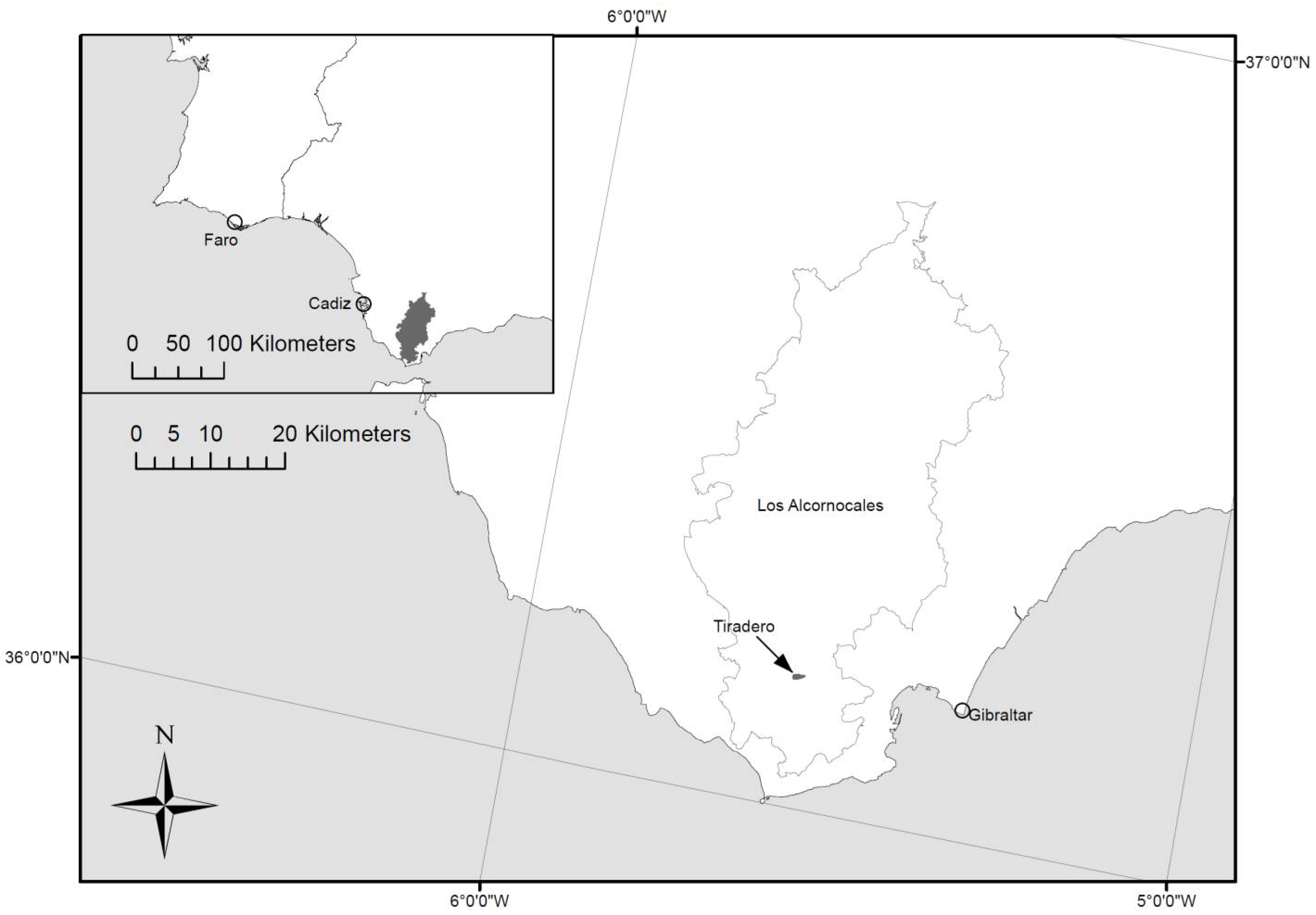
2.1. Study Area

The Sierra del Aljibe is a range of mountains rising to 1092 m and protected within the Los Alcornocales Natural Park. It represents an edaphic island of sandstone-derived acidic and nutrient-poor soils surrounded by base-rich soils of limestone, marl and clay. The area contains the most extensive Quercus suber (cork oak) forest in Iberia and the Mediterranean region. This evergreen oak forms mixed and segregated patches with the co-dominant Algerian oak semi-deciduous Quercus canariensis, which occupies moister valleys and north-facing slopes.
Within the Park, our research is focused on a site of mixed closed-canopy forest (approximate area 93 ha) at Tiradero (36° 09′38′′N, 5° 35′25′′W; 335–360 m a.s.l.; Figure 1) on a gentle northeast facing slope. This is a reserve set aside from management and therefore unaffected by the widespread understorey cutting that is commonly associated with cork harvest, pasture improvement and fire control. Herbivory levels are high, however, and there is a small amount of disturbance from the maintenance and use of a marked hiking trail, as well as scientific research.

2.2. Field Survey

Field sampling of the forest at Tiradero was undertaken in April, May and September 2011. Plant communities were sampled within 28 circular 10 m radius plots in a grid of seven (east–west orientation) by four (north–south), as ground truthing in support of an investigation into topographic and canopy controls on understories [27]. Plots were located using a GPSMAP 60CSx (Garmin, Olathe, KS, USA), with a horizontal accuracy of 3 m; errors in the colocation of field and remotely sensed data had previously been found to be negligible using this system in cork oak woodlands [28]. Vegetation vertical profiles were constructed from plant contacts with a vertical pole at 20 random locations and five height intervals within each plot. Cover abundance values were assigned to all non-graminoid vascular plant species according to the Braun Blanquet five-point scale [29]. The number of individuals of each tree species within the plot was recorded, and basal area calculated from diameter-at-breast height (DBH) measurements for trees of DBH > 10 cm. Whilst these data were collected in support of research into canopy–understorey linkages described by [27], they provide contextual information to help interpret the results of this current study. Data from two plots in particular were used for this purpose (Figure 2 and Section 2.5).

2.3. LiDAR Survey

Data acquisition for an area encompassing the Tiradero study site took place on 10 April 2011. A total of sixteen east–west overlapping strips of approximate length 8 km and width 600 m were surveyed from an altitudinal range of 929–953 m above ground level. A coverage of approximately 50 km2, in the coordinate space 36°08′–36°11′N, 5°32′–5°37′W (UTM WGS84 zone 30N) was thus achieved. The Leica ALS50 LiDAR operates at a wavelength of 1064 nm with a pulse frequency of 86 kHz, pulse density of c 2.5 m−2, and footprint diameter of approximately 13 cm resulting from the combination of instrument operating parameters (Table 1). Vertical placement accuracy of this instrument is <10 cm for the survey flying altitude [30]. Simultaneous GPS measurement was carried out on the ground using a Leica dGPS1200, as an adjustment of permanent GPS station calibration data obtained from Cadiz (SFER) and Ceuta (CEU1). Further LiDAR data were collected on 22 May 2011, i.e., 42 days after the first survey, due to patchy cloud cover leading to incomplete coverage of another section of the study area. The temporal analysis described here is based on a comparison of the data from one of the new (May) east–west strips, and an original (April) one to which it overlapped almost exactly. The viewing angle range for the study area was therefore identical, and at a maximum of 10° not considered likely to have a major impact on the height-based measurements [31,32]. For both flights, Specimen Eagle and Hawk hyperspectral imagers were also in operation, and a Leica RCD105 39 megapixel camera produced digital photographic coverage. The latter images were useful for distinguishing the main areas of Q. suber and Q. canariensis dominated canopy, with seasonal true-colour differences reflecting changes in the leafing state of these two trees (Figure 2).

2.4. LiDAR Data Processing

Post-flight processing of the LiDAR data was carried out by NERC’s Remote Sensing Group at the Plymouth Marine Laboratory. Modelling of terrain and canopy heights was performed using the software ‘Tiffs’ 8.0: Toolbox for Lidar Data Filtering and Forest Studies ([33]; Globalidar 2006–2011). After importing and tiling data strips, the Tiffs core function is to filter the point cloud into ground and non-ground returns. A morphological filtering method described by [34] is employed, and, being grid-based, it is computationally efficient and fast. For each tile, the outputs from the filtering process were Digital Elevation Models (DEMs), Digital Surface Models (DSMs), and Object Height Models (OHMs) at a spatial resolution of 5 m, as well as ground, object (vegetation) and combined point data. We employed the DEM from a single LiDAR acquisition (that for April) for both time points, following the precedent of previous multi-temporal studies [35].
The Tiffs software facilitates individual tree as well as grid-based analyses. Its marker-controlled watershed segmentation method [36] was used to identify treetops and crown boundaries of trees for tiles covering the Tiradero core study area. The software also extracts structural parameters for the trees, calculated from the normalised vegetation heights (all returns). The statistics that were calculated were maximum, mean, standard deviation, quadratic mean, skewness and kurtosis of vegetation heights, and crown radius and canopy volume (being the volume under the OHM for the delineated tree crown [37]). The simultaneous grid-based statistical analysis (GSA) returned the same set of height metrics (excluding crown dimensions) for cells of size 5 m.

2.5. Temporal Analysis

We wanted to compare the effect of acquisition date on the LiDAR measurement of forest structure, at both the tree crown and 5 m grid cell level. Metrics were retrieved from surveys on 10 April 2011 and 22 May 2011, an interval of 42 days. This interval spans a period of significant leaf change for the two dominant trees of the mixed forest study area: the evergreen cork oak Quercus suber undergoes both leaf loss and emergence, whilst the semi-deciduous Q. canariensis is in a state of leaf expansion. The comparisons were made for a 20 ha area of mixed forest, and two smaller (2 ha) areas contained therein, differing in their predominant canopy type: Quercus suber versus Quercus canariensis (Figure 2). The areas used in the comparisons were drawn as quadrilateral polygons in ArcGIS, and were used to extract the sets of tree- and grid-level data from the shapefiles of wider coverage.
For the comparison of LiDAR statistics of individual trees, the package spatstat [38] implemented in R language (R Development Core Team 2012) was used to match trees identified in one survey with trees identified in the next. Spatstat is designed for analysing spatial point patterns. For two point patterns A and B, its function nncross computes the nearest neighbour in B for each point of A. For our purposes, we applied nncross to associate trees isolated from the one LiDAR object height model (OHM) to the assumed same trees isolated from the second LiDAR OHM. Distances between A and B will be small when the same tree is detected in the two surveys. Once trees had been matched, the ratio of values for each of the eight LiDAR statistics was calculated and analysed according to distance between the neighbours (corresponding to amount of error in the localisation of trees). In the absence of phenology-related changes, ratios are expected to equal 1 (the measured values do not change between surveys) when trees are perfectly matched (A–B distance values are low).
Comparable grid-based analyses were conducted based on raster files of 5 m cell size clipped by the 20 ha and 2 ha areas of interest. In this case, ratios of change of four LiDAR variables (maximum, mean, standard deviation and skewness of vegetation heights) were calculated between surveys. The ratio values (April/May), for both grid cells and trees, were tested for significant difference from the value 1 using Wilcoxon signed rank tests for non-normal data.
To aid the interpretation of the results, the same four LiDAR variables compared in the grid-cell analysis were also calculated from the LiDAR vegetation point data extracted for two circular plots of radius 10 m, for which field data on vegetation vertical profile and plant community composition were available (see Section 2.2). The two plots chosen comprised one for each of the two main canopy types, and were the ones nearest to the two 2-ha study areas (Figure 2). The LiDAR point clouds for these plots were inspected using the data exploration tool Treevis (version 0.78, University of Freiburg, Germany), as well as the graphing of scatterplots. Such visualisation and inspection of the data can prove highly useful in the detection of patterns and relationships [39].

3. Results

3.1. Selection of Trees

April–May comparisons were made on eight LiDAR metrics calculated for segmented trees crowns (Figure 3), and four metrics for 5 m grid cells (Figure 4). Temporal differences in the metrics increased with offset distance between matched trees in the near-neighbour analysis (Supplementary Materials, Figure S1), although this effect was clearer with some metrics (e.g., mean and quadratic mean) than others (e.g., crown dimensions). Further consideration of the tree data is therefore restricted to trees matched with most certainty, taken to be within 2 m (representing approximately 60% of the total segmented trees, or 2900 comparisons for the 20 ha plot and c. 300 comparisons for the 2 ha plots).

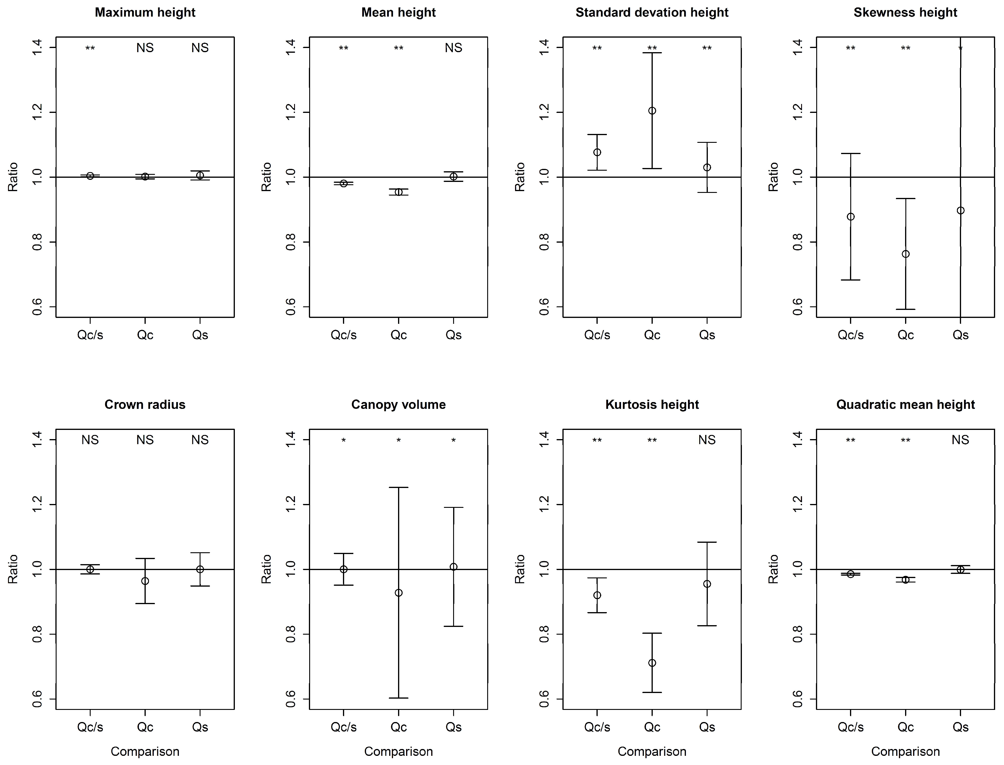
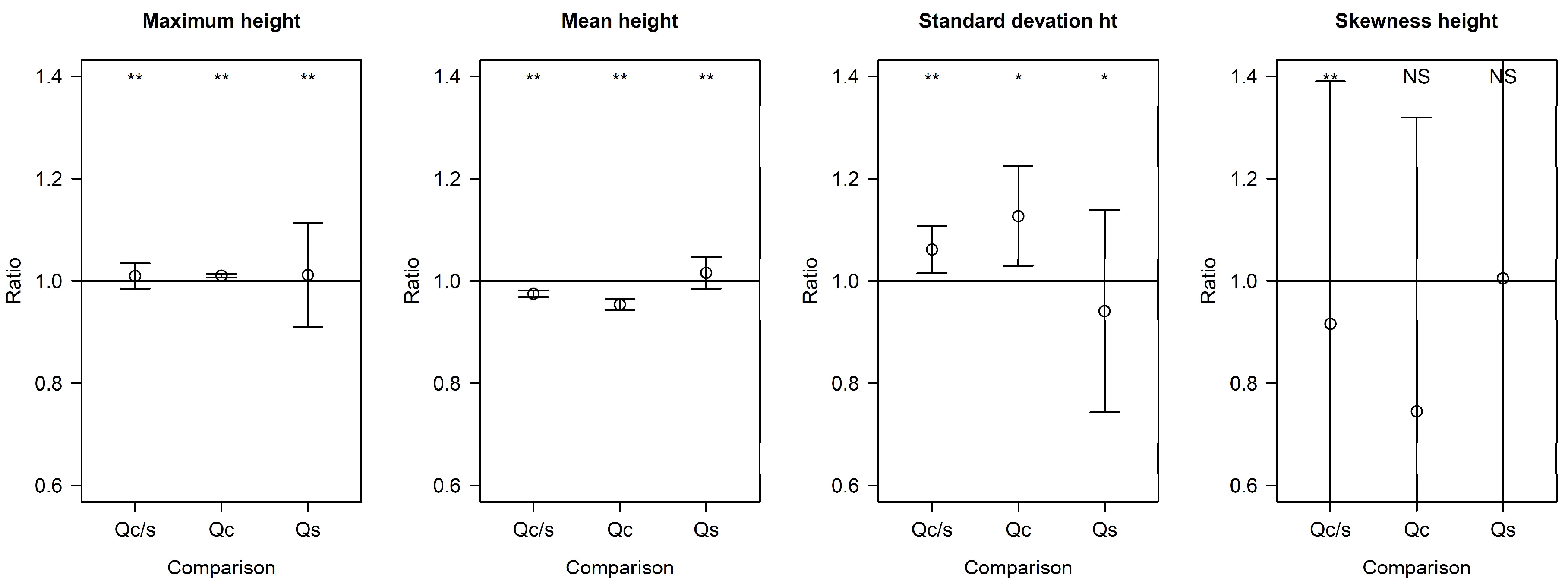
3.2. April–May Comparison of LiDAR Metrics

We predicted that April–May comparisons of LiDAR metrics would reveal significant differences as a result of phenological changes to leafing state and this was demonstrated for the majority of the metrics by the significant deviation of the April–May ratios from the value 1 (Figure 3 and Figure 4).
The variable that differed least between surveys was maximum height: ratio values in both tree and grid analyses were very close to the value of 1 (Figure 3 and Figure 4, Supplementary Materials Figure S1). The tree analysis also revealed only small differences in the measurement of mean height between surveys (Figure 3); for the grid analysis, the May measurements of mean height were higher for the mixed plot and Q. canariensis (Figure 4). For the standard deviation of heights, ratio values > 1 were evident in nearly all comparisons (Figure 3 and Figure 4). Of all metrics included in the tree and grid cell analyses, skewness values were most dissimilar across surveys, and also variable in that dissimilarity. The results at the tree level showed lower skewness in May than in April (all values are negative, hence in this case a lower ratio value corresponds to a more negative value in May). For the four metrics studied in the tree analysis alone, crown radius, crown volume and quadratic mean height had very similar values in the comparisons, whilst kurtosis values increased from April to May (Figure 3).

3.3. Canopy Species-Specific Effects

An effect of canopy type was clearly observed in the April–May comparisons (Figure 3 and Figure 4). We hypothesised that, in the case of Quercus canariensis, which undergoes leaf expansion during the study period, the reduced penetration of LiDAR pulses through the canopy in May would lead to greater April–May differences in metric retrieval compared to Q. suber. The results, at both tree and grid-cell level, confirmed this prediction. For the semi-deciduous tree in the tree analysis, the increase in mean height and reduced standard deviation and skewness of heights in May compared to April were more marked than for Q. suber (Figure 3). This was evident for the 2-ha Q. canariensis plot and the 20-ha plot as a whole, which had a predominance of this tree. For both the tree and grid analyses, skewness of height in Q. canariensis canopies was at least 20% less in May compared to April, the differences for Q. suber being much less (Figure 3 and Figure 4).
In relation to the Q. suber canopy, the April survey was undertaken at the onset of rapid leaf drop, whilst the May survey was carried out during the spring flush of new leaf growth. The digital imagery, with variation in the hue of green, suggests that full leaf expansion had not been achieved in all trees (Figure 2). As such, the net change in foliage mass and volume is less easy to predict, and the tree and grid analyses produce inconsistent support for either an increase or decrease in interception of the laser pulses at the canopy level. The slightly lower mean height value for May in the grid analysis (Figure 4) would suggest reduced foliage and more penetration of the laser through the canopy, and this is consistent with a higher standard deviation of heights for the second survey. In the tree analysis, skewness of heights experiences a significant reduction in May (Figure 3), whilst also a reduced standard deviation of heights.
The distribution of height measurements for the two example circular plots helps to interpret differences exhibited by Quercus canariensis and Q. suber (Figure 5 and Table 2). In the Q. suber plot, the abundance of undershrubs to a height of 2 m is captured in both strips. This was mostly composed of the shrubs Erica arborea and Genista triacanthos and liane Smilax aspera. A relatively unfilled space apparently sits below the Q. suber canopy. For the Q. canariensis plot, a taller, shallower but potentially denser canopy is suggested by the scatterplots. Field records suggest some presence of Q. suber and Phillyrea latifolia, and this is reflected by the scatter of returns at 4 m and above. A lower understorey of Ruscus aculeatus, Smilax aspera, Myrtus communis and other shrubs is also suggested. Notably, the sub-canopy vegetation (7 m and below) appears less well captured in the May survey. Comparisons of the four LiDAR variables were remarkably consistent for both plots (Table 2), with the ratio value falling in the range 0.95–1.03, with the exception of the skewness of heights for Q. suber, and both skewness and standard deviation of heights for Q. canariensis.

4. Discussion

A chief strength of our approach is that the repeat surveys are conducted using the same sensor configuration and flight parameters, and in the same year. Despite obvious advantages, this has rarely been possible in past multi-temporal LiDAR studies. Data collection in a mixed deciduous woodland in eastern England [16] was separated by two years, as was the case in a study in southeast Norway [11]. The experimental design of the latter investigation was also undertaken with different sensors at different flying altitudes, requiring a number of complicated compensations in the analysis. Flying altitude can have a significant effect, as a reduction in peak pulse power concentration can delay pulse triggering within vegetation, thereby increasing laser penetration into the foliage and reducing height metric values [40]. An increased interval time, on the other hand, allows tree growth to become a factor.
This investigation has found evidence for the effect of seasonality, specifically short-term spring-time leafing phenology in two typical Mediterranean forest species, on the retrieval of LiDAR variables of value for describing tree crown and forest stand vegetation structural attributes. In this way, the specific contribution that the study makes is in the investigation of more subtle effects of tree leafing phenology than the often studied leaf-on/leaf-off dichotomy. The investigation was opportunistic upon an unplanned repeat LiDAR survey, and hence a campaign of field data collection aimed at quantifying the associated phenological changes was not planned. We have, however, been able to draw upon contextual field data to reach some robust conclusions on the effect of seasonal tree leafing processes and the retrieval of LiDAR metrics.
Airborne LiDAR is being increasingly applied in Mediterranean ecosystems (e.g., [41,42,43,44,45,46,47]). Knowledge of the effect on LiDAR parameters of seasonal changes to these predominantly evergreen canopies—including climatic influences on leafing phenology—is relevant to the design, data-analysis and interpretation of LiDAR surveys in this and other warm-temperate/sub-tropical regions.
Contrasting responses were observed for Quercus canariensis and Quercus suber canopies, according to our hypothesis. Field observation and comparison of the digital imagery for April and May (Figure 2) indicate that the Quercus canariensis trees develop from a state of partial to full leaf expansion during this period. Under partial leaf expansion, reflectances off branches will presumably represent a relatively high proportion of the LiDAR point cloud. As leaves expand, one can predict that the increased amount of foliage biomass, and canopy closure, will reduce penetration of laser pulses and increase the proportion and concentration of height measurements recorded in the upper strata of the vegetation profile. Our results confirmed this prediction, with an increased mean height, reduced standard deviation and more negative skewness of heights, in May compared to April. These results are analogous to those found for leaf-on/leaf-off conditions. For lowland mixed woodlands in eastern England, a small increase in mean height (13.35 vs. 12.47 m) and decrease in standard deviation of heights (5.10 vs. 5.25 m) was observed in leaf-on conditions [16]. The height distributions of single returns and last-of-many returns have been shown to shift towards the ground in leaf-off conditions within boreal forests [10]; skewness values under leaf-off conditions were more positive for single returns (but not for first or last returns) and the variability of the height distribution tended to increase from leaf-on to leaf-off conditions. In another study, the laser interception by the upper parts of a mixed forest canopy were significantly higher in leaf-on conditions [11]. For the first return data, height metrics were 0.33–0.97 m higher under leaf-on canopy conditions. Analogous results were also shown in a comparison between tropical moist (TMF) and tropical wet (TWF) forest [48]. At the end of the dry season, leaf loss from canopy-forming trees was pronounced in some TMF areas, and this led to less LiDAR energy being reflected from the upper canopy, thereby reducing the LiDAR median height metric relative to the TWF study area. In an investigation of light availability at different developmental stages of a boreal forest [49], a direct relationship between skewness and the degree of light entering through crown was established, results that are consistent with the canopy closure between April and May in our study forest.
Maximum height was the least variable of the four metrics for Quercus canariensis plots. The ratio values of ~1 for maximum height measurement for trees and grid cells is reassuring, in terms of reliable measurement of a variable that should be less affected by tree leafing phenology than the others that were calculated. This is again consistent with the results of the studies that have been reviewed here. Leaf-on/leaf-off values in one investigation were 25.31/25.14 m [16]. In another, canopy conditions were found to exert little influence on the maximum height obtained for the individual trees, although maximum laser heights of ‘first’ echoes were higher in birch trees under leaf-off conditions [10]. Meanwhile, plot-level stability of maximum height has been reported [11]. Using percentile heights, a tendency for canopy height to be underestimated in leaf-off conditions has been observed, but only where the forest was dominated by deciduous compound-leaved trees [14].
The tree-level and grid analyses have complemented each other in the comparison of time periods and canopy types. The former provided a number of metrics associated with tree crowns, whilst the latter was unaffected by any error in the tree segmentation process. The results of both give confidence that the LiDAR variables are relatively robust to the seasonality of tree leafing that this study spans. A possible exception is the measurement of skewness, especially in the case of the Q. canariensis canopy, and the reasons for this have already been discussed. Skewness of heights is a useful summary measure of their asymmetry as affected by canopy closure [49] and relative density of vegetation in the canopy and understorey layers. It can be used, for example, to differentiate natural forest and plantations, with their varying vertical vegetation profiles [50]. The reduced skewness values obtained for Q. canariensis plots during the May survey suggests that this timing is less optimal to capture information on the presence of understorey vegetation. This may also be the case for the evergreen Q. suber, though evidence for this from our study is equivocal. It may be that a survey undertaken later in the summer, with full leafing out of the cork oak trees, would similarly be less useful for the description of layers below the tree canopy.

5. Conclusions

This investigation has provided a unique record of the effect of within-season tree leafing state on the consistency of LiDAR measurement of mixed evergreen/semi-deciduous forests. It provides reassurance that retrieval of standard parameters such as maximum and mean height of trees are robust to a degree of leaf expansion, but that care in the timing of a survey is required when sub-canopy vegetation layers—being relevant, for example, to modelling fire fuel loads—are the focus of investigation, particularly for trees of a more deciduous nature. For the area studied in this current investigation, the earlier spring-time canopy state of April was preferential for detecting an adequate signal of the sub-canopy strata, especially in the patches dominated by the deciduous Quercus canariensis. If the modelling of the canopy surface alone is important, the robustness of the maximum height LiDAR metric would suggest that the survey timing is not critical.

Supplementary Materials

The following are available online at https://www.mdpi.com/2072-4292/10/5/659/s1.

Author Contributions

W.S. and D.C. conceived and designed the methodological approach; W.S., H.A. and D.C. undertook the field data collection; W.S. performed the remote sensing data analysis; W.S. wrote the paper and H.A. and D.C. provided inputs and comments on the drafts.

Acknowledgments

Data acquisition was performed by the Airborne Research and Survey Facility, NERC (project EU11/03), and access to the Tiradero study site arranged by Manuela Malla of the Los Alcornocales Natural Park office. We are grateful for the cooperation of all involved. Our thanks to Ruben Valbuena for comments on an earlier draft of this paper.

Conflicts of Interest

The authors declare no conflict of interest.

References

  1. Lefsky, M.; Cohen, W.B.; Acker, S.A.; Parker, G.G.; Spies, T.A.; Harding, D. Lidar Remote Sensing of the Canopy Structure and Biophysical Properties of Douglas-Fir Western Hemlock Forests. Remote Sens. Environ. 1999, 70, 339–361. [Google Scholar] [CrossRef]
  2. Lim, K.; Treitz, P.; Wulder, M.; St-Onge, B.; Flood, M. LiDAR remote sensing of forest structure. Prog. Phys. Geogr. 2003, 27, 88–106. [Google Scholar] [CrossRef]
  3. Danson, F.M.; Morsdorf, F.; Koetz, B. Airborne and terrestrial laser scanning for measuring vegetation canopy structure. In Laser Scanning for the Environmental Sciences; Heritage, G., Large, A., Eds.; Wiley-Blackwell: Oxford, UK, 2009; pp. 201–219. [Google Scholar]
  4. Broughton, R.K.; Hinsley, S.A.; Bellamy, P.E.; Hill, R.A.; Rothery, P. Marsh Tit Poecile palustris territories in a British broad-leaved wood. Ibis 2006, 148, 744–752. [Google Scholar] [CrossRef]
  5. Graf, R.; Mathys, L.; Bollmann, K. Habitat assessment for forest dwelling species using LiDAR remote sensing: Capercaillie in the Alps. For. Ecol. Manag. 2009, 257, 160–167. [Google Scholar] [CrossRef]
  6. Goetz, S.J.; Steinberg, D.; Betts, M.G.; Holmes, R.T.; Doran, P.J.; Dubayah, R.; Hofton, M. Lidar remote sensing variables predict breeding habitat of a Neotropical migrant bird. Ecology 2010, 91, 1569–1576. [Google Scholar] [CrossRef] [PubMed]
  7. Asner, G.P. Tropical forest carbon assessment: Integrating satellite and airborne mapping approaches. Environ. Res. Lett. 2009, 4, 1–11. [Google Scholar] [CrossRef]
  8. Saatchi, S.S.; Harris, N.L.; Brown, S.; Lefsky, M.; Mitchard, E.T.A.; Salas, W.; Zutta, B.R.; Buermann, W.; Lewis, S.L.; Hagen, S.; et al. Benchmark map of forest carbon stocks in tropical regions across three continents. Proc. Natl. Acad. Sci. USA 2011, 108, 9899–9904. [Google Scholar] [CrossRef] [PubMed]
  9. Korpela, I.; Hovi, A.; Korhonen, L. Backscattering of individual LiDAR pulses from forest canopies explained by photogrammetrically derived vegetation structure. ISPRS J. Photogramm. Remote Sens. 2013, 83, 81–93. [Google Scholar] [CrossRef]
  10. Orka, H.O.; Næsset, E.; Bollandsås, O.M. Effects of different sensors and leaf-on and leaf-off canopy conditions on echo distributions and individual tree properties derived from airborne laser scanning. Remote Sens. Environ. 2010, 114, 1445–1461. [Google Scholar] [CrossRef]
  11. Næsset, E. Assessing sensor effects and effects of leaf-off and leaf-on canopy conditions on biophysical stand properties derived from small-footprint airborne laser data. Remote Sens. Environ. 2005, 98, 356–370. [Google Scholar] [CrossRef]
  12. Kim, S.; McGaughey, R.J.; Andersen, H.-E.; Schreuder, G. Tree species differentiation using intensity data derived from leaf-on and leaf-off airborne laser scanner data. Remote Sens. Environ. 2009, 113, 1575–1586. [Google Scholar] [CrossRef]
  13. Villikka, M.; Packalén, P.; Maltamo, M. The suitability of leaf-off airborne laser scanning data in an area-based forest inventory of coniferous and deciduous trees. Silva Fenn. 2012, 46, 99–110. [Google Scholar] [CrossRef]
  14. Wasser, L.; Day, R.; Chasmer, L.; Taylor, A. Influence of Vegetation Structure on Lidar-derived Canopy Height and Fractional Cover in Forested Riparian Buffers During Leaf-Off and Leaf-On Conditions. PLoS ONE 2013, 8, e54776. [Google Scholar] [CrossRef] [PubMed]
  15. White, J.C.; Arnett, J.T.T.R.; Wulder, M.A.; Tompalski, P.; Coops, N.C. Evaluating the impact of leaf-on and leaf-off airborne laser scanning data on the estimation of forest inventory attributes with the area-based approach. Can. J. For. Res. 2015, 1513, 1498–1513. [Google Scholar] [CrossRef]
  16. Hill, R.A.; Broughton, R.K. Mapping the understorey of deciduous woodland from leaf-on and leaf-off airborne LiDAR data: A case study in lowland Britain. ISPRS J. Photogramm. Remote Sens. 2009, 64, 223–233. [Google Scholar] [CrossRef]
  17. Hirata, Y.; Sato, K.; Shibata, M.; Nishizono, T. The capability of helicopter-borne laser scanner data in a temperate deciduous forest. In Proceedings of the Workshop Scandlaser Scientific Workshop on Airborne Laser Scanning of Forests, Umea, Sweden, 3–4 September 2003; Hyyppä, J., Naesset, E., Olsson, H., Granqvist Phalén, T., Reese, H., Eds.; Instutionen för Skoglig Resurshushållning, Sveriges Lantbruksuniversitet: Umeå, Sweden, 2003; pp. 174–179. [Google Scholar]
  18. Thomas, P.A.; Packham, J.R. Ecology of Woodlands and Forests; Cambridge University Press: Cambridge, UK, 2007. [Google Scholar]
  19. Zhao, K.; Suarez, J.C.; Garcia, M.; Hu, T.; Wang, C.; Londo, A. Utility of multitemporal lidar for forest and carbon monitoring: Tree growth, biomass dynamics, and carbon flux. Remote Sens. Environ. 2018, 204, 883–897. [Google Scholar] [CrossRef]
  20. Vepakomma, U.; St-Onge, B.; Kneeshaw, D. Spatially explicit characterization of boreal forest gap dynamics using multi-temporal lidar data. Remote Sens. Environ. 2008, 112, 2326–2340. [Google Scholar] [CrossRef]
  21. Næsset, E.; Bollandsås, O.M.; Gobakken, T.; Gregoire, T.G.; Ståhl, G. Model-assisted estimation of change in forest biomass over an 11 year period in a sample survey supported by airborne LiDAR: A case study with post-stratification to provide “activity data”. Remote Sens. Environ. 2013, 128, 299–314. [Google Scholar] [CrossRef]
  22. Huang, C.; Wylie, B.; Yang, L.; Homer, C.; Zylstra, G. Derivation of a tasselled cap transformation based on Landsat 7 at-satellite reflectance. Int. J. Remote Sens. 2002, 23, 1741–1748. [Google Scholar] [CrossRef]
  23. Hopkinson, C.; Chasmer, L.; Hall, R.J. The uncertainty in conifer plantation growth prediction from multi-temporal lidar datasets. Remote Sens. Environ. 2008, 112, 1168–1180. [Google Scholar] [CrossRef]
  24. Dubayah, R.O.; Sheldon, S.L.; Clark, D.B.; Hofton, M.A.; Blair, J.B.; Hurtt, G.C.; Chazdon, R.L. Estimation of tropical forest height and biomass dynamics using lidar remote sensing at La Selva, Costa Rica. J. Geophys. Res. 2010, 115, G00E09. [Google Scholar] [CrossRef]
  25. Simonson, W.; Ruiz-Benito, P.; Valladares, F.; Coomes, D. Modelling above-ground carbon dynamics using multi-temporal airborne lidar: Insights from a Mediterranean woodland. Biogeosciences 2016, 13, 961–973. [Google Scholar] [CrossRef]
  26. Jenkins, R.B. Airborne laser scanning for vegetation structure quantification in a south east Australian scrubby forest-woodland. Austral Ecol. 2012, 37, 44–55. [Google Scholar] [CrossRef]
  27. Simonson, W.D.; Allen, H.D.; Coomes, D.A. Overstorey and topographic effects on understories: Evidence for linkage from cork oak (Quercus suber) forests in southern Spain. For. Ecol. Manag. 2014, 328, 35–44. [Google Scholar] [CrossRef]
  28. Simonson, W.D.; Allen, H.D.; Coomes, D.A. Use of an Airborne Lidar System to Model Plant Species Composition and Diversity of Mediterranean Oak Forests. Conserv. Biol. 2012, 26, 840–850. [Google Scholar] [CrossRef] [PubMed]
  29. Sutherland, W.J. Ecological Census Techniques, A Handbook; Cambridge University Press: Cambridge, UK, 1996. [Google Scholar]
  30. Leica Leica ALS50-II Product Specifications. Available online: http://www.nts-info.com/inventory/images/ALS50-II.Ref.703.pdf (accessed on 4 April 2018).
  31. Holmgren, J.; Nilsson, M.; Olsson, H. Simulating the effects of lidar scanning angle for estimation of mean tree height and canopy closure. Can. J. Remote Sens. 2003, 29, 623–632. [Google Scholar] [CrossRef]
  32. Morsdorf, F.; Frey, O.; Meier, E.; Itten, K.I.; Allgöwer, B. Assessment of the influence of flying altitude and scan angle on biophysical vegetation products derived from airborne laser scanning. Int. J. Remote Sens. 2008, 1161, 1387–1406. [Google Scholar] [CrossRef]
  33. Chen, Q. Airborne Lidar Data Processing and Information Extraction. Photogramm. Eng. Remote Sens. 2007, 73, 109–112. [Google Scholar]
  34. Chen, Q.; Gong, P.; Baldocchi, D.; Xie, G. Filtering Airborne Laser Scanning Data with Morphological Methods. Photogramm. Eng. Remote Sens. 2007, 73, 175–185. [Google Scholar] [CrossRef]
  35. Yu, X.; Hyyppä, J.; Kaartinen, H.; Maltamo, M. Automatic detection of harvested trees and determination of forest growth using airborne laser scanning. Remote Sens. Environ. 2004, 90, 451–462. [Google Scholar] [CrossRef]
  36. Chen, Q.; Baldocchi, D.; Gong, P.; Kelly, M. Isolating Individual Trees in a Savanna Woodland Using Small Footprint Lidar Data. Photogramm. Eng. Remote Sens. 2006, 72, 923–932. [Google Scholar] [CrossRef]
  37. Chen, Q.; Gong, P.; Baldocchi, D.; Tian, Y.Q. Estimating Basal Area and Stem Volume for Individual Trees from Lidar Data. Photogramm. Eng. Remote Sens. 2007, 73, 1355–1365. [Google Scholar] [CrossRef]
  38. Baddeley, A.; Turner, R. Spatstat: An R package for analyzing spatial point patterns. J. Stat. Softw. 2005, 12, 1–42. [Google Scholar] [CrossRef]
  39. Cleveland, W.S. Rejoinder: A model for studying display methods of statistical graphics. J. Comput. Graph. Stat. 1993, 2, 361–364. [Google Scholar]
  40. Hopkinson, C. The influence of flying altitude, beam divergence, and pulse repetition frequency on laser pulse return intensity and canopy frequency distribution. Can. J. Remote Sens. 2007, 33, 312–324. [Google Scholar] [CrossRef]
  41. Riaño, D.; Valladares, F.; Condés, S.; Chuvieco, E. Estimation of leaf area index and covered ground from airborne laser scanner (Lidar) in two contrasting forests. Agric. For. Meteorol. 2004, 124, 269–275. [Google Scholar] [CrossRef]
  42. Riaño, D.; Meier, E.; Allgower, B.; Chuvieco, E.; Ustin, S.L. Modeling airborne laser scanning data for the spatial generation of critical forest parameters in fire behavior modeling. Remote Sens. Environ. 2003, 86, 177–186. [Google Scholar] [CrossRef]
  43. Riaño, D.; Chuvieco, E.; Ustin, S.L.; Salas, J.; Rodríguez-Pérez, J.R.; Ribeiro, L.M.; Viegas, D.X.; Moreno, J.M.; Fernández, H. Estimation of shrub height for fuel-type mapping combining airborne LiDAR and simultaneous color infrared ortho imaging. Int. J. Wildl. Fire 2007, 16, 341–348. [Google Scholar] [CrossRef]
  44. García, M.; Riaño, D.; Chuvieco, E.; Danson, F.M. Estimating Biomass Carbon Stocks for a Mediterranean Forest in Central Spain Using LiDAR Height and Intensity Data. Remote Sens. Environ. 2010, 114, 816–830. [Google Scholar] [CrossRef]
  45. García, M.; Riaño, D.; Chuvieco, E.; Salas, J.; Danson, F.M. Multispectral and LiDAR data fusion for fuel type mapping using Support Vector Machine and decision rules. Remote Sens. Environ. 2011, 115, 1369–1379. [Google Scholar] [CrossRef]
  46. Morsdorf, F.; Mårell, A.; Koetz, B.; Cassagne, N.; Pimont, F.; Rigolot, E.; Allgöwer, B. Discrimination of vegetation strata in a multi-layered Mediterranean forest ecosystem using height and intensity information derived from airborne laser scanning. Remote Sens. Environ. 2010, 114, 1403–1415. [Google Scholar] [CrossRef] [Green Version]
  47. Ferraz, A.; Bretar, F.; Jacquemoud, S.; Gonçalves, G.; Pereira, L.; Tomé, M.; Soares, P. 3-D mapping of a multi-layered Mediterranean forest using ALS data. Remote Sens. Environ. 2012, 121, 210–223. [Google Scholar] [CrossRef]
  48. Drake, J.B.; Knox, R.G.; Dubayah, R.O.; Clark, D.B.; Condit, R.; Blair, J.B.; Hofton, M. Above-ground biomass estimation in closed canopy Neotropical forests using lidar remote sensing: Factors affecting the generality of relationships. Glob. Ecol. Biogeogr. 2003, 12, 147–159. [Google Scholar] [CrossRef]
  49. Valbuena, R.; Maltamo, M.; Mehtätalo, L.; Packalen, P. Key structural features of Boreal forests may be detected directly using L-moments from airborne lidar data. Remote Sens. Environ. 2017, 194, 437–446. [Google Scholar] [CrossRef]
  50. Antonarakis, A.S.; Richards, K.S.; Brasington, J. Object-based land cover classification using airborne LiDAR. Remote Sens. Environ. 2008, 112, 2988–2998. [Google Scholar] [CrossRef]
Figure 1. The study area located in the Los Alcornocales Natural Park, which is to be found in the Andalucia region of southwest Spain (inset).
Remotesensing 10 00659 g001
Figure 2. The 20-ha study site (in white), with Quercus suber (left, in yellow) and Quercus canariensis (right, in yellow) 2-ha sub-areas and representative 10-m radius field plots (black circles, see Section 2.2). Digital photography of the tree canopy on 10 April (top) and 22 May 2011 (bottom) is from a Leica RCD105 39 megapixel camera (Wetzlar, Germany).
Remotesensing 10 00659 g002
Figure 3. Bar plots showing LiDAR April/May measurement ratios (with 95% confidence intervals) for eight tree statistics. Results of Wilcoxon signed rank tests of significant difference from the value 1 are given above each bar (** significant at p = 0.01; * significant at p = 0.05; N.S. not significant.) Results for the 20 ha mixed Q. canariensis/suber plot (Qc/s), 2 ha Q. canariensis (Qc) and Q. suber (Qs) plots are given.
Remotesensing 10 00659 g003
Figure 4. Bar plots showing LiDAR April/May measurement ratios (with 95% confidence intervals) for four 5 m grid-cell statistics: maximum, mean, standard deviation and skewness. Results of Wilcoxon signed rank tests of significant difference from the value 1 are given above each bar (** significant at p = 0.01; * significant at p = 0.05; N.S. not significant.) Results for the 20 ha mixed Q. canariensis/suber plot (Qc/s), 2 ha Q. canariensis (Qc) and Q. suber (Qs) plots are given.
Remotesensing 10 00659 g004
Figure 5. Scatterplots of vegetation heights for two representative circular plots of radius 10 m: Quercus suber dominated plot (top row) and Q. canariensis dominated plot (bottom row). Filled symbols are first returns, and open symbols second and third returns.
Remotesensing 10 00659 g005
Table 1. Specifications for the LiDAR surveys undertaken in the Tiradero study area, Los Alcornocales, 2011.
April SurveyMay Survey
LiDAR sensorLeica ALS050Leica ALS050
Date of deployment10 April 201122 May 2011
Align in12:4809:16
Ground speed135–148 knots141–150 knots
Flight altitude (above ground)929–953 m938–960 m
Pulse rate frequency85.1–86.1 MHz86.1–89.9 MHz
Field of view (degrees)1212
Scan frequency54.8 Hz54.8–57.4 Hz
Number of strips16 (E–W) + 1 (N–S)2 (E–W) + 1 (N–S)
Wavelength1064 nm1064 nm
Beam divergence0.22 mrad0.22 mrad
Footprint size13 cm13 cm
Vertical discrimination 2.8 m2.8 m
Detection systemFour returnFour return
Table 2. Average values of four LiDAR metrics for the two representative 10 m radius circular plots differing by canopy type, as well as ratio values for April–May comparisons.
Metric Values
Canopy TypeHeight Statistic (m)AprilMayApril–May Ratio Value
Quercus suberMaximum10.6510.291.03
Mean6.285.941.06
Standard deviation2.802.890.97
Skewness−1.01−0.911.11
Quercus canariensisMaximum14.9614.851.01
Mean9.8310.160.97
Standard deviation3.362.931.15
Skewness−1.35−1.620.83

