Multi-Temporal DInSAR to Characterise Landslide Ground Deformations in a Tropical Urban Environment: Focus on Bukavu (DR Congo)

 , , and
Abstract
:
1. Introduction
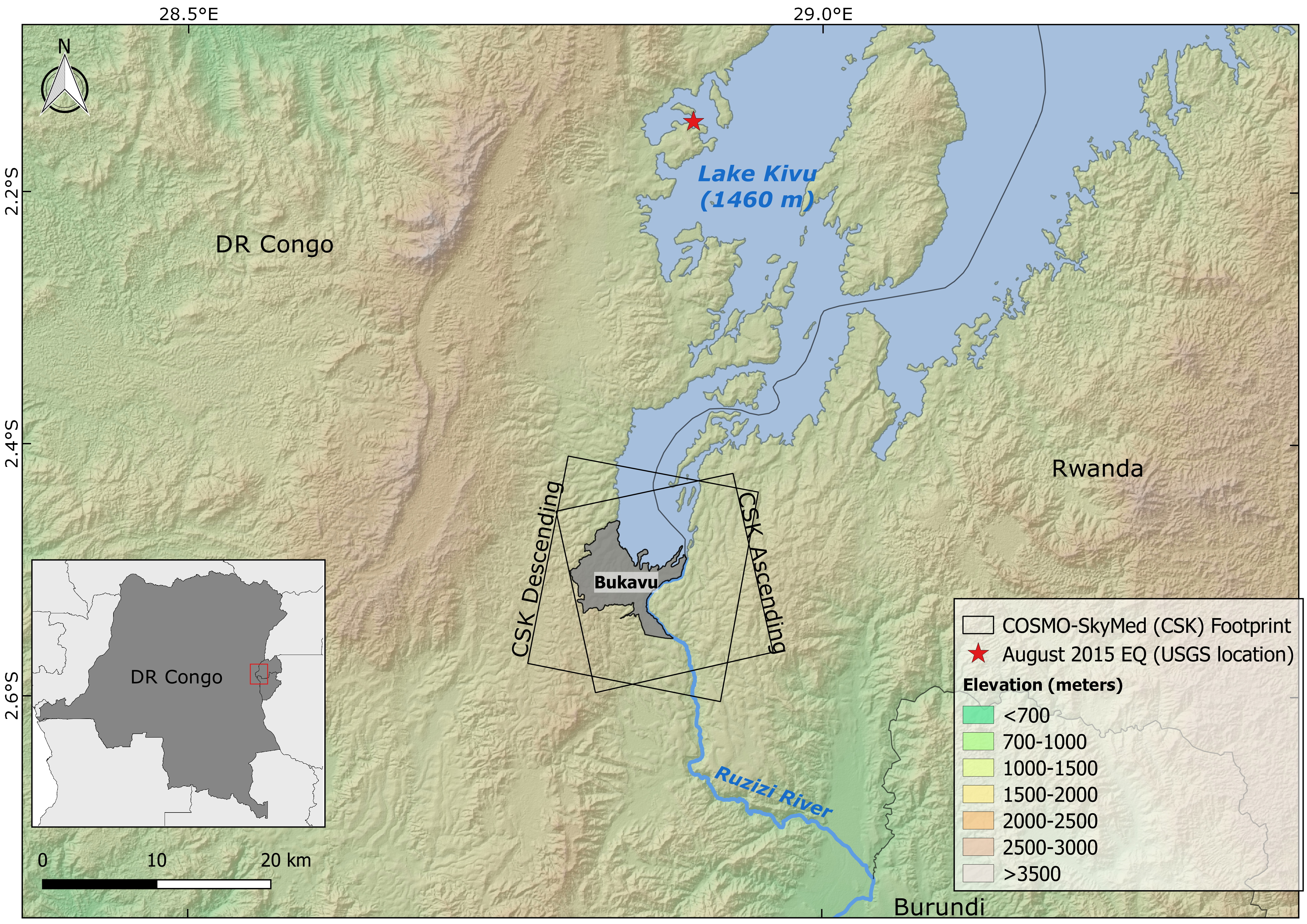
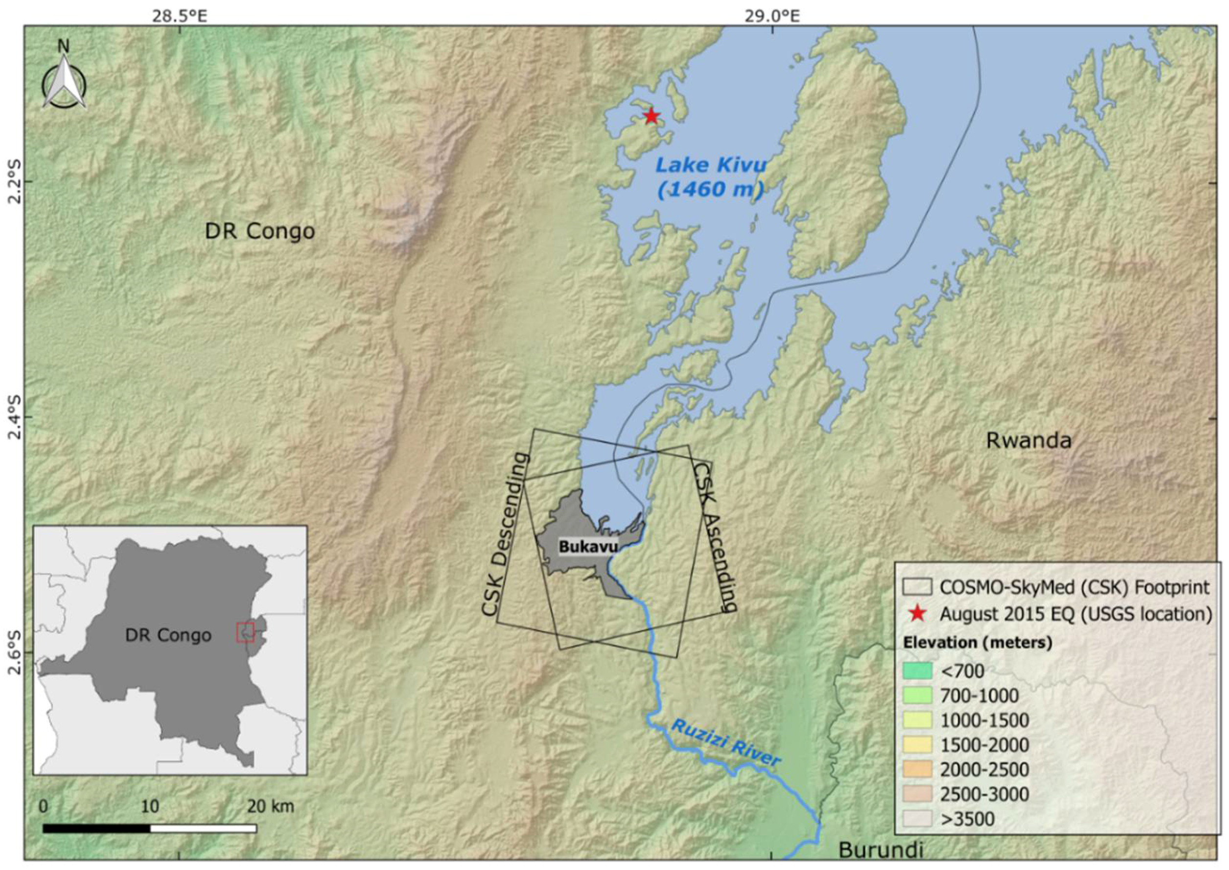
2. Study Area
3. Materials and Methods
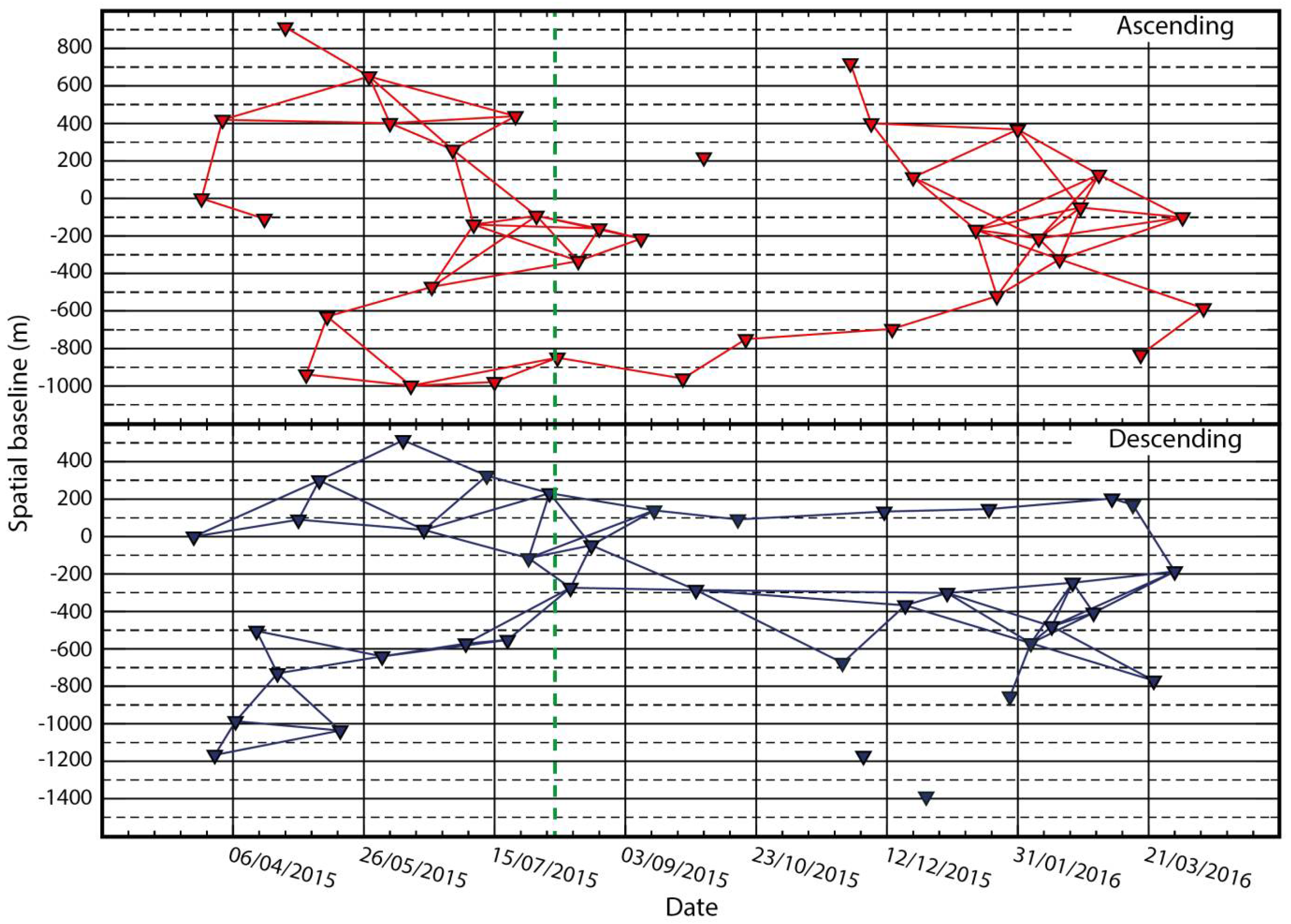
3.1. SAR Data and DInSAR Processing
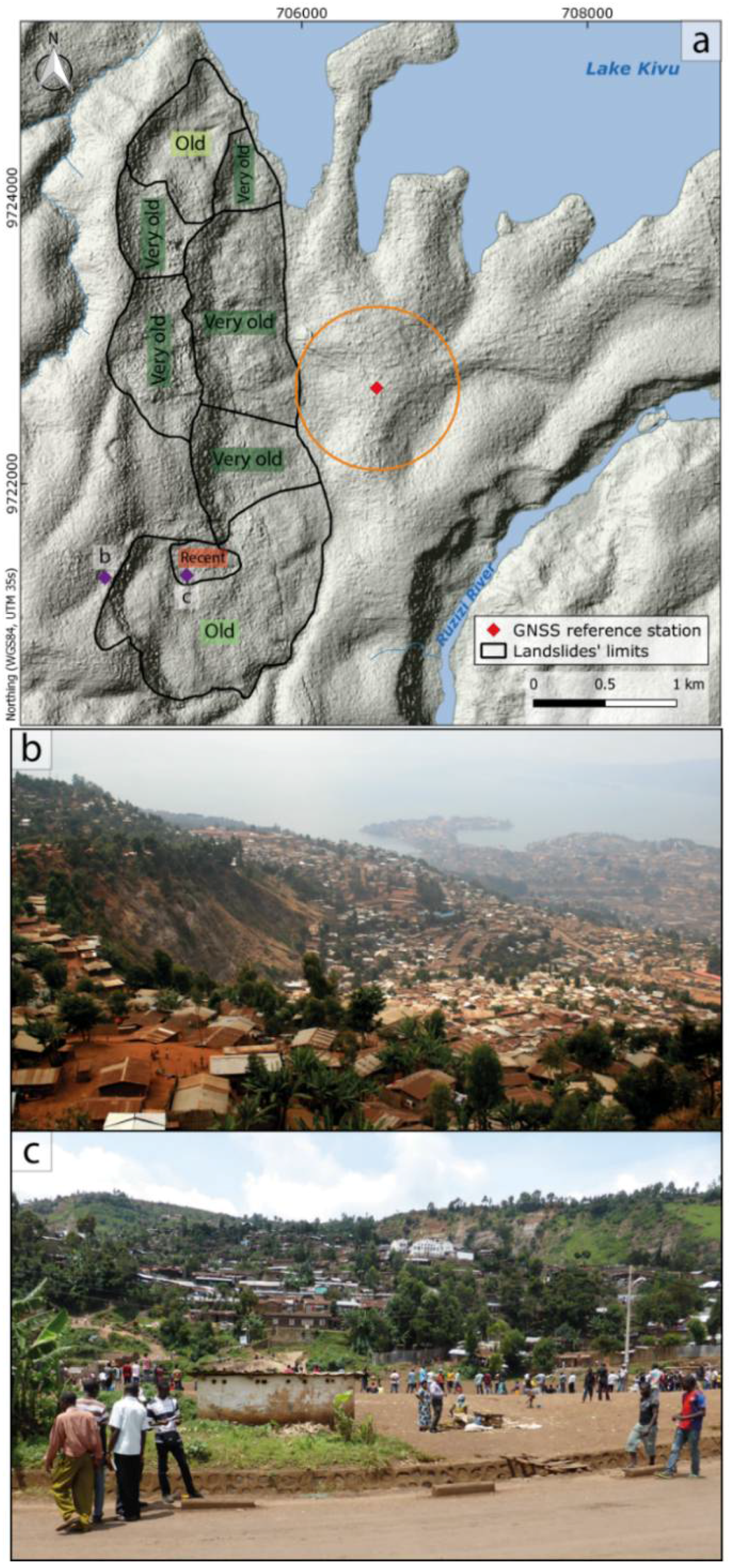
3.2. Geomorphological Landslide Inventory
3.3. DGPS Measurements
4. Results
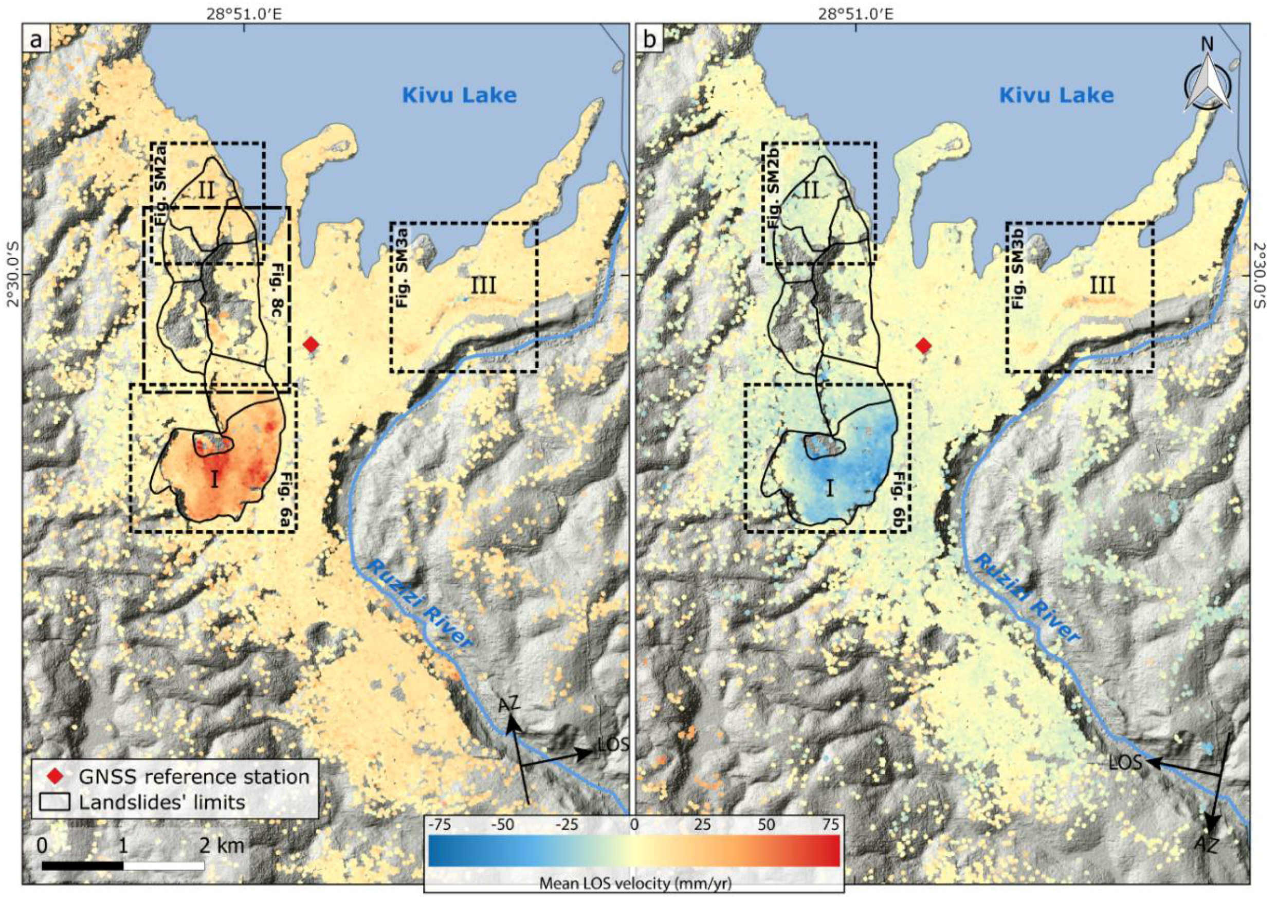
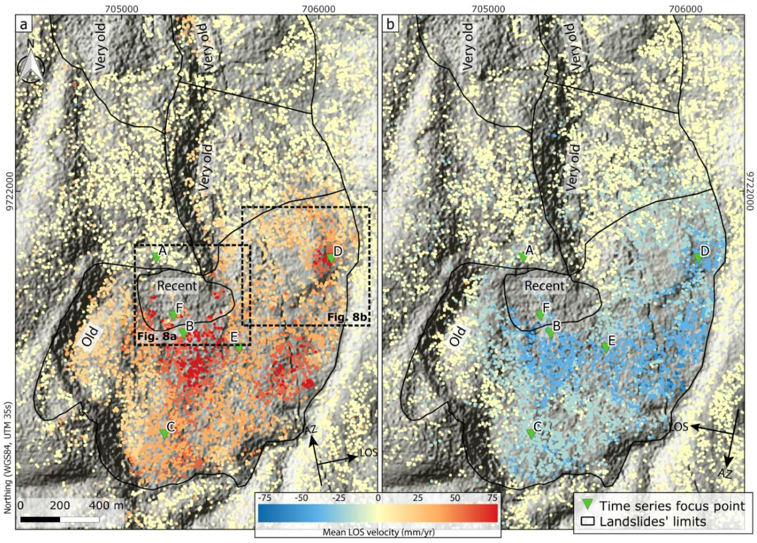
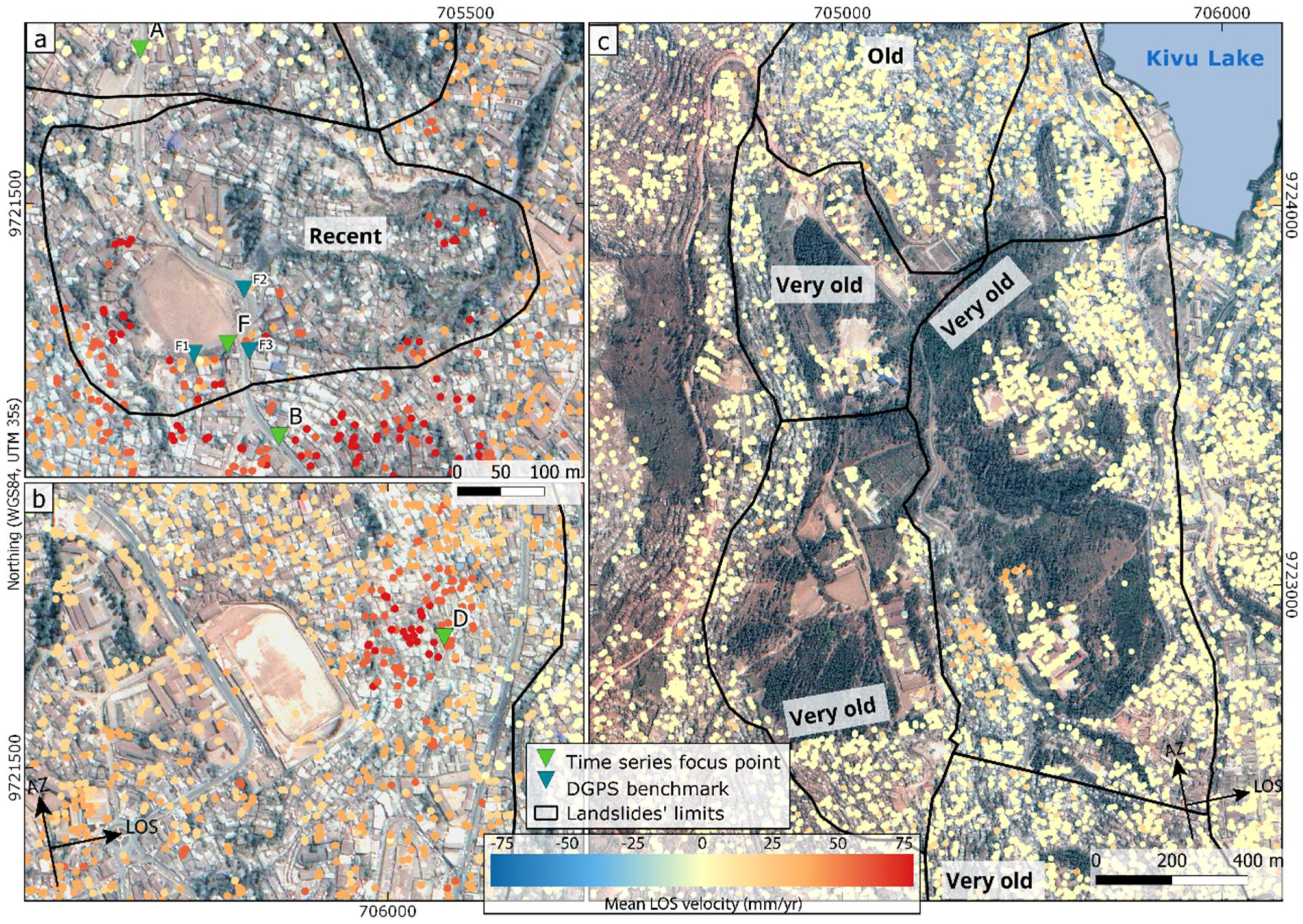
4.1. DInSAR Ground Deformations
4.2. Comparison of DInSAR Ground Deformations to the Landslide Inventory
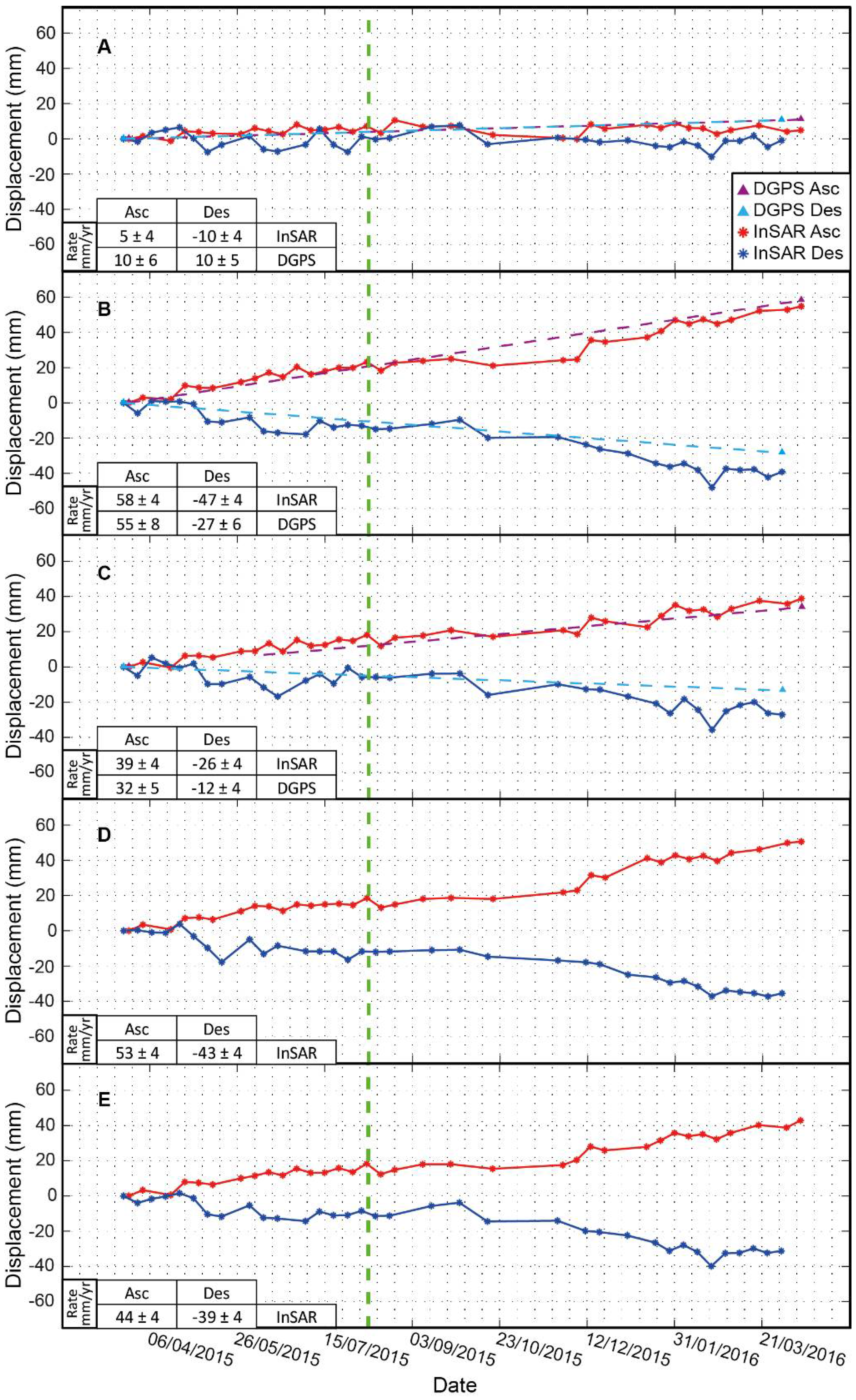
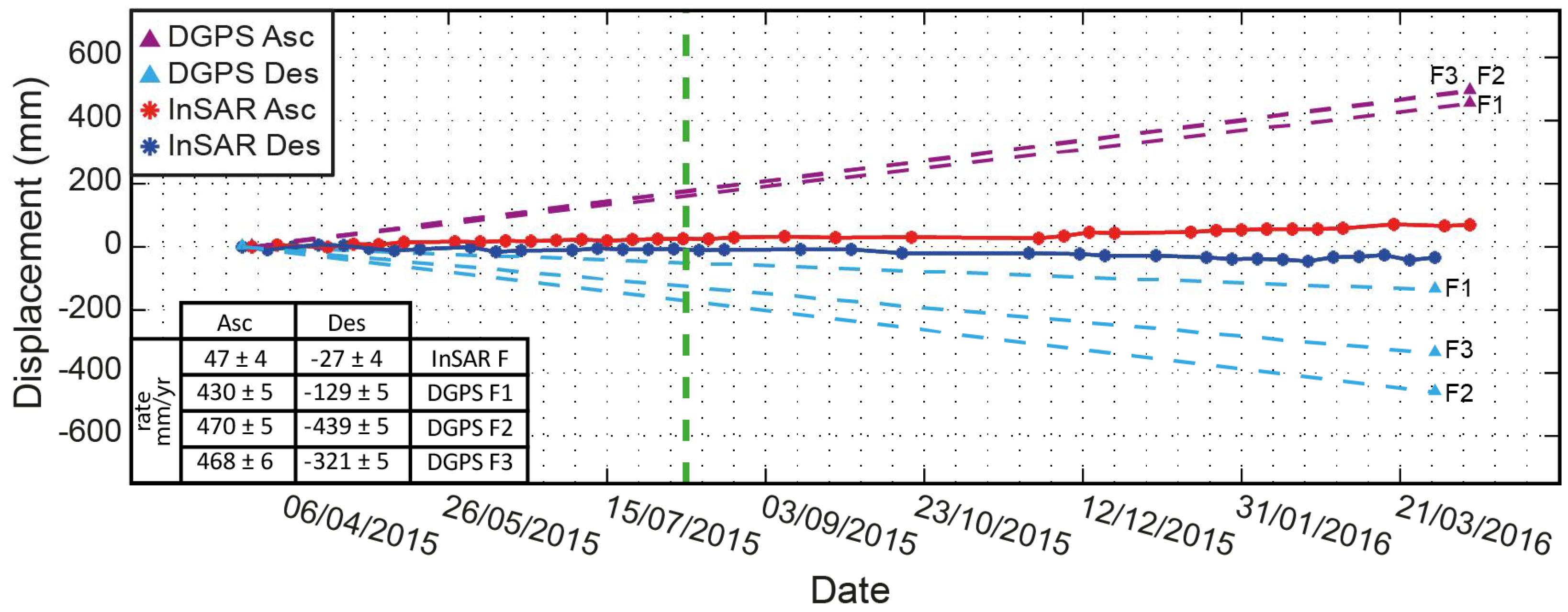
4.3. Comparison of DInSAR Ground Deformations to DGPS Measurements
5. Discussion
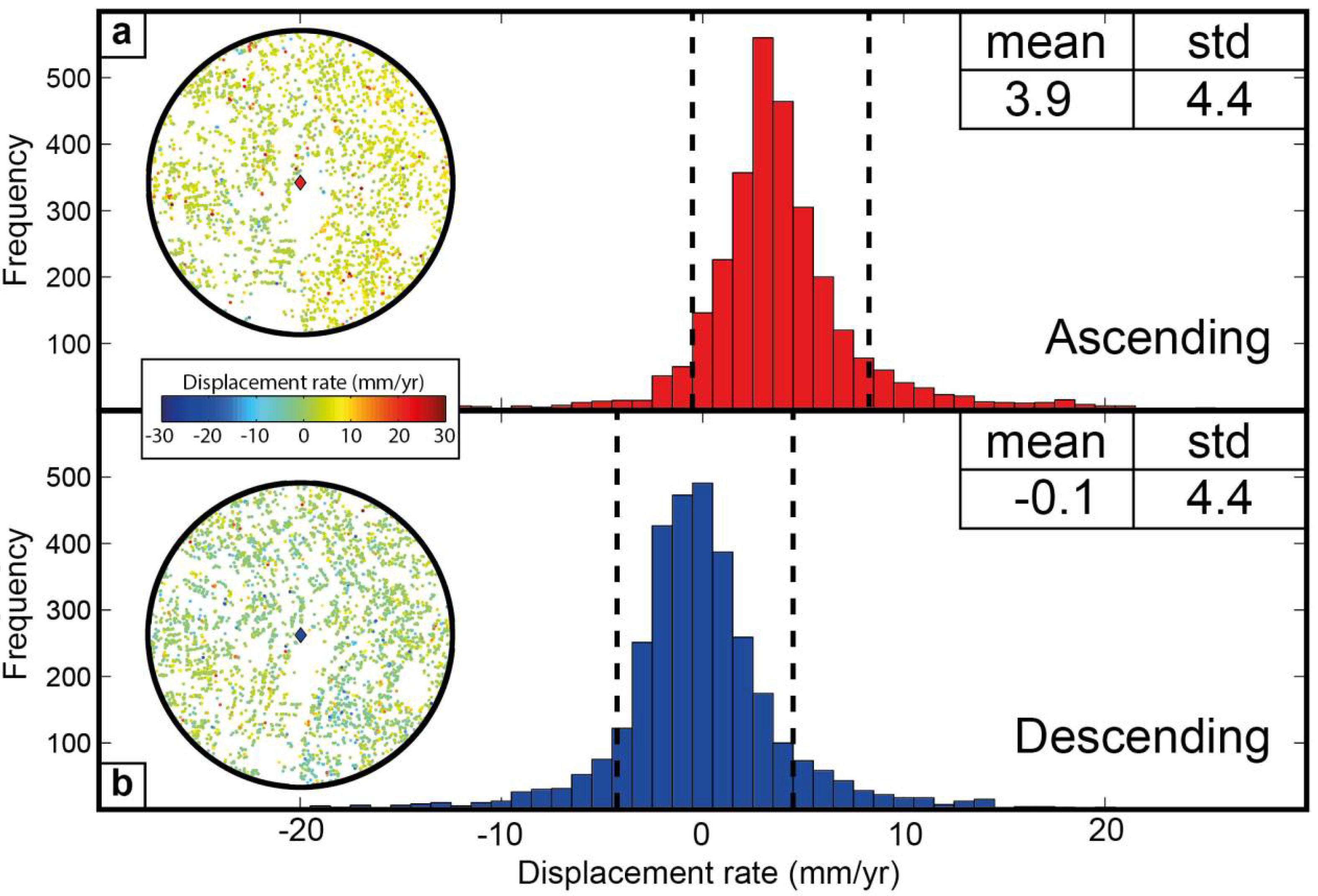
5.1. Reliability of DInSAR Measurements
5.2. DInSAR Deformation Time Series and Landslide Processes
5.3. Limitations of the DInSAR Technique for Landslide Characterisation
6. Conclusions
Supplementary Materials
Acknowledgments
Author Contributions
Conflicts of Interest
References
- Jacobs, L.; Dewitte, O.; Poesen, J.; Delvaux, D.; Thiery, W.; Kervyn, M. The Rwenzori Mountains, a landslide-prone region? Landslides 2016, 13, 519–536. [Google Scholar] [CrossRef]
- Kirschbaum, D.; Stanley, T.; Zhou, Y. Spatial and temporal analysis of a global landslide catalog. Geomorphology 2015, 249, 4–15. [Google Scholar] [CrossRef]
- Monsieurs, E.; Kirschbaum, D.; Thiery, W.; van Lipzig, N.; Kervyn, M.; Demoulin, A.; Jacobs, L.; Kervyn, F.; Dewitte, O. Constraints on Landslide-Climate Research Imposed by the Reality of Fieldwork in Central Africa. In Proceedings of the 3rd North American Symposium Landslides, Landslides: Putting Experience, Knowledge and Emerging Technologies into Practice, Roanoke, VA, USA, 4–8 June 2017; pp. 158–168. [Google Scholar]
- Petley, D. Global patterns of loss of life from landslides. Geology 2012, 40, 927–930. [Google Scholar] [CrossRef]
- Sidle, R.C.; Ziegler, A.D.; Negishi, J.N.; Nik, A.R.; Siew, R.; Turkelboom, F. Erosion processes in steep terrain—Truths, myths, and uncertainties related to forest management in Southeast Asia. For. Ecol. Manag. 2006, 224, 199–225. [Google Scholar] [CrossRef]
- DeFries, R.S.; Rudel, T.; Uriarte, M.; Hansen, M. Deforestation driven by urban population growth and agricultural trade in the twenty-first century. Nat. Geosci. 2010, 3, 178–181. [Google Scholar] [CrossRef]
- Gariano, S.L.; Guzzetti, F. Landslides in a changing climate. Earth-Sci. Rev. 2016, 162, 227–252. [Google Scholar] [CrossRef]
- Maes, J.; Kervyn, M.; de Hontheim, A.; Dewitte, O.; Jacobs, L.; Mertens, K.; Vanmaercke, M.; Vranken, L.; Poesen, J. Landslide risk reduction measures: A review of practices and challenges for the tropics. Prog. Phys. Geogr. 2017, 41, 191–221. [Google Scholar] [CrossRef]
- Knapen, A.; Kitutu, M.G.; Poesen, J.; Breugelmans, W.; Deckers, J.; Muwanga, A. Landslides in a densely populated county at the footslopes of Mount Elgon (Uganda): Characteristics and causal factors. Geomorphology 2006, 73, 149–165. [Google Scholar] [CrossRef]
- Schulz, W.H.; Coe, J.A.; Ricci, P.P.; Smoczyk, G.M.; Shurtleff, B.L.; Panosky, J. Landslide kinematics and their potential controls from hourly to decadal timescales: Insights from integrating ground-based InSAR measurements with structural maps and long-term monitoring data. Geomorphology 2017, 285, 121–136. [Google Scholar] [CrossRef]
- Bennett, G.L.; Roering, J.J.; Mackey, B.H.; Handwerger, A.L.; Schmidt, D.A.; Guillod, B.P. Historic drought puts the brakes on earthflows in Northern California. Geophys. Res. Lett. 2016, 43, 5725–5731. [Google Scholar] [CrossRef]
- Schlögel, R.; Doubre, C.; Malet, J.P.; Masson, F. Landslide deformation monitoring with ALOS/PALSAR imagery: A D-InSAR geomorphological interpretation method. Geomorphology 2015, 231, 314–330. [Google Scholar] [CrossRef]
- Stumpf, A.; Malet, J.-P.; Delacourt, C. Correlation of satellite image time-series for the detection and monitoring of slow-moving landslides. Remote Sens. Environ. 2017, 189, 40–55. [Google Scholar] [CrossRef]
- Reiche, J.; Lucas, R.; Mitchell, A.L.; Verbesselt, J.; Hoekman, D.H.; Haarpaintner, J.; Kellndorfer, J.M.; Rosenqvist, A.; Lehmann, E.A.; Woodcock, C.E.; et al. Combining satellite data for better tropical forest monitoring. Nat. Clim. Chang. 2016, 6, 120–122. [Google Scholar] [CrossRef]
- Ferretti, A.; Prati, C.; Rocca, F. Permanent Scatters in SAR Interferometry. IEEE Trans. Geosci. Remote Sens. 2001, 39, 8–20. [Google Scholar] [CrossRef]
- Crosetto, M.; Monserrat, O.; Devanthéry, N.; Cuevas-González, M.; Barra, A.; Crippa, B. Persistent scatterer interferometry using Sentinel-1 data. Int. Arch. Photogramm. Remote Sens. Spat. Inf. Sci. ISPRS Arch. 2016, 41, 835–839. [Google Scholar] [CrossRef]
- Berardino, P.; Fornaro, G.; Lanari, R.; Sansosti, E. A new algorithm for surface deformation monitoring based on small baseline differential SAR interferograms. IEEE Trans. Geosci. Remote Sens. 2002, 40, 2375–2383. [Google Scholar] [CrossRef]
- Lanari, R.; Casu, F.; Manzo, M.; Zeni, G.; Berardino, P.; Manunta, M.; Pepe, A. An overview of the Small BAseline Subset algorithm: A DInSAR technique for surface deformation analysis. Pure Appl. Geophys. 2007, 164, 637–661. [Google Scholar] [CrossRef]
- Colesanti, C.; Wasowski, J. Investigating landslides with space-borne Synthetic Aperture Radar (SAR) interferometry. Eng. Geol. 2006, 88, 173–199. [Google Scholar] [CrossRef]
- Wasowski, J.; Bovenga, F. Investigating landslides and unstable slopes with satellite Multi Temporal Interferometry: Current issues and future perspectives. Eng. Geol. 2014, 174, 103–138. [Google Scholar] [CrossRef]
- Raspini, F.; Bardi, F.; Bianchini, S.; Ciampalini, A.; Del Ventisette, C.; Farina, P.; Ferrigno, F.; Solari, L.; Casagli, N. The contribution of satellite SAR-derived displacement measurements in landslide risk management practices. Nat. Hazards 2017, 86, 327–351. [Google Scholar] [CrossRef]
- Bovenga, F.; Pasquariello, G.; Pellicani, R.; Re, A.; Spilotro, G. Landslide monitoring for risk mitigation by using corner reflector and satellite SAR interferometry: The large landslide of Carlantino (Italy). Catena 2017, 151, 49–62. [Google Scholar] [CrossRef]
- Mirzaee, S.; Motagh, M.; Akbari, B.; Wetzel, H.U.; Roessner, S. Evaluating Three InSAR Time-Series Methods To Assess Creep Motion, Case Study: Masouleh Landslide in North Iran. ISPRS Ann. Photogramm. Remote Sens. Spat. Inf. Sci. 2017, IV-1/W1, 223–228. [Google Scholar] [CrossRef]
- Bayer, B.; Simoni, A.; Mulas, M.; Corsini, A.; Schmidt, D. Deformation responses of slow moving landslides to seasonal rainfall in the Northern Apennines, measured by InSAR. Geomorphology 2018. [Google Scholar] [CrossRef]
- Prati, C.; Ferretti, A.; Perissin, D. Recent advances on surface ground deformation measurement by means of repeated space-borne SAR observations. J. Geodyn. 2010, 49, 161–170. [Google Scholar] [CrossRef]
- Hooper, A.; Bekaert, D.; Spaans, K.; Arikan, M. Recent advances in SAR interferometry time series analysis for measuring crustal deformation. Tectonophysics 2012, 514–517, 1–13. [Google Scholar] [CrossRef]
- Bekaert, D.P.S.S.; Walters, R.J.; Wright, T.J.; Hooper, A.J.; Parker, D.J. Statistical comparison of InSAR tropospheric correction techniques. Remote Sens. Environ. 2015, 170, 40–47. [Google Scholar] [CrossRef]
- Bovenga, F.; Wasowski, J.; Nitti, D.O.; Nutricato, R.; Chiaradia, M.T. Using COSMO/SkyMed X-band and ENVISAT C-band SAR interferometry for landslides analysis. Remote Sens. Environ. 2012, 119, 272–285. [Google Scholar] [CrossRef]
- Notti, D.; Davalillo, J.C.; Herrera, G.; Mora, O. Assessment of the performance of X-band satellite radar data for landslide mapping and monitoring: Upper Tena Valley case study. Nat. Hazards Earth Syst. Sci. 2010, 10, 1865–1875. [Google Scholar] [CrossRef] [Green Version]
- Calò, F.; Ardizzone, F.; Castaldo, R.; Lollino, P.; Tizzani, P.; Guzzetti, F.; Lanari, R.; Angeli, M.G.; Pontoni, F.; Manunta, M. Enhanced landslide investigations through advanced DInSAR techniques: The Ivancich case study, Assisi, Italy. Remote Sens. Environ. 2014, 142, 69–82. [Google Scholar] [CrossRef]
- Cigna, F.; Bateson, L.B.; Jordan, C.J.; Dashwood, C. Simulating SAR geometric distortions and predicting Persistent Scatterer densities for ERS-1/2 and ENVISAT C-band SAR and InSAR applications: Nationwide feasibility assessment to monitor the landmass of Great Britain with SAR imagery. Remote Sens. Environ. 2014, 152, 441–466. [Google Scholar] [CrossRef]
- Milillo, P.; Fielding, E.J.; Shulz, W.H.; Delbridge, B.; Burgmann, R. COSMO-skymed spotlight interferometry over rural areas: The slumgullion landslide in Colorado, USA. IEEE J. Sel. Top. Appl. Earth Obs. Remote Sens. 2014, 7, 2919–2926. [Google Scholar] [CrossRef]
- Novellino, A.; Cigna, F.; Sowter, A.; Ramondini, M.; Calcaterra, D. Exploitation of the Intermittent SBAS (ISBAS) algorithm with COSMO-SkyMed data for landslide inventory mapping in north-western Sicily, Italy. Geomorphology 2017, 280, 153–166. [Google Scholar] [CrossRef]
- Elliott, J.R.; Walters, R.J.; Wright, T.J. The role of space-based observation in understanding and responding to active tectonics and earthquakes. Nat. Commun. 2016, 7, 13844. [Google Scholar] [CrossRef] [PubMed]
- Crosetto, M.; Copons, R.; Cuevas-González, M.; Devanthéry, N.; Monserrat, O. Monitoring soil creep landsliding in an urban area using persistent scatterer interferometry (El Papiol, Catalonia, Spain). Landslides 2018, 1983. [Google Scholar] [CrossRef]
- Moeyersons, J.; Tréfois, P.; Lavreau, J.; Alimasi, D.; Badriyo, I.; Mitima, B.; Mundala, M.; Munganga, D.O.; Nahimana, L. A geomorphological assessment of landslide origin at Bukavu, Democratic Republic of the Congo. Eng. Geol. 2004, 72, 73–87. [Google Scholar] [CrossRef]
- Trefois, P.; Moeyersons, J.; Lavreau, J.; Alimasi, D.; Badryio, I.; Mitima, B.; Mundala, M.; Munganga, D.O.; Nahimana, L. Geomorphology and urban geology of Bukavu (R.D. Congo): Interaction between slope instability and human settlement. Geol. Soc. Lond. Spec. Publ. 2007, 283, 65–75. [Google Scholar] [CrossRef]
- Michellier, C.; Delvaux, D.; D’Oreye, N.; Dewitte, O.; Havenith, H.-B.; Kervyn, M.; Poppe, S.; Trefon, T.; Wolff, E.; Kervyn, F. Geo-Risk in Central Africa: Integrating Multi-Hazards and Vulnerability to Support Risk Management; Final Report; Belgian Science Policy: Brussels, Belgium, 2018; pp. 1–186. [Google Scholar]
- Michellier, C.; Pigeon, P.; Kervyn, F.; Wolff, E. Contextualizing vulnerability assessment: A support to geo-risk management in central Africa. Nat. Hazards 2016, 82, 27–42. [Google Scholar] [CrossRef]
- Eriksen, H.Ø.; Lauknes, T.R.; Larsen, Y.; Corner, G.D.; Bergh, S.G.; Dehls, J.F. Visualizing Surface Displacement Patterns Using Multi-Geometry Satellite SAR Interferometry. Remote Sens. Environ. 2017, 191, 297–312. [Google Scholar] [CrossRef]
- D’Oreye, N.; González, P.J.; Shuler, A.; Oth, A.; Bagalwa, L.; Ekström, G.; Kavotha, D.; Kervyn, F.; Lucas, C.; Lukaya, F.; et al. Source parameters of the 2008 Bukavu-Cyangugu earthquake estimated from InSAR and teleseismic data. Geophys. J. Int. 2011, 184, 934–948. [Google Scholar] [CrossRef] [Green Version]
- Delvaux, D.; Mulumba, J.-L.; Sebagenzi, M.N.S.; Bondo, S.F.; Kervyn, F.; Havenith, H.-B. Seismic hazard assessment of the Kivu rift segment based on a new seismotectonic zonation model (western branch, East African Rift system). J. Afr. Earth Sci. 2016. [Google Scholar] [CrossRef]
- Hooper, A.J. A multi-temporal InSAR method incorporating both persistent scatterer and small baseline approaches. Geophys. Res. Lett. 2008, 35, 1–5. [Google Scholar] [CrossRef]
- Biggs, J.; Wright, T.; Lu, Z.; Parsons, B. Multi-interferogram method for measuring interseismic deformation: Denali Fault, Alaska. Geophys. J. Int. 2007, 170, 1165–1179. [Google Scholar] [CrossRef]
- Ding, X.L.; Li, Z.W.; Zhu, J.J.; Feng, G.C.; Long, J.P. Atmospheric effects on InSAR measurements and their mitigation. Sensors 2008, 8, 5426–5448. [Google Scholar] [CrossRef] [PubMed]
- Zebker, H.A.; Villasenor, J. Decorrelation in Inteferometric Radar Echoes. IEEE Trans. Geosci. Remote Sens. 1992, 30, 950–959. [Google Scholar] [CrossRef]
- Crosetto, M.; Monserrat, O.; Cuevas-González, M.; Devanthéry, N.; Crippa, B. Persistent Scatterer Interferometry: A review. ISPRS J. Photogramm. Remote Sens. 2016, 115, 78–89. [Google Scholar] [CrossRef]
- Hooper, A.; Bekaert, D.; Spaans, K. StaMPS/MTI Manual; School of Earth and Environment, University of Leeds: Leeds, UK, 2013. [Google Scholar]
- Farr, T.G.; Kobrick, M. Shuttle radar topography mission produces a wealth of data. EOS Trans. Am. Geophys. Union 2000, 81, 583–585. [Google Scholar] [CrossRef]
- Goldstein, R.M.; Werner, C.L. Radar interferogram filtering for geophysical applications. Geophys. Res. Lett. 1998, 25, 4035–4038. [Google Scholar] [CrossRef]
- Hooper, A.; Zebker, H.A. Phase unwrapping in three dimensions with application to InSAR time series. J. Opt. Soc. Am. A 2007, 24, 2737. [Google Scholar] [CrossRef]
- Geirsson, H.; d’Oreye, N.; Mashagiro, N.; Syauswa, M.; Celli, G.; Kadufu, B.; Smets, B.; Kervyn, F. Volcano-tectonic deformation in the Kivu Region, Central Africa: Results from six years of continuous GNSS observations of the Kivu Geodetic Network (KivuGNet). J. Afr. Earth Sci. 2016. [Google Scholar] [CrossRef]
- Burgmann, R.; Rosen, P.A.; Fielding, E.J. Synthetic Aperture Radar Interferometry to Measure Earth’s Surface Topography and its Defromation. Annu. Rev. Earth Planet. Sci. 2000, 28, 169–209. [Google Scholar] [CrossRef]
- Hanssen, R.F. Radar Interferometry: Data Interpretation and Error Analysis; Springer Science & Business Media: Berlin, Germany, 2001; ISBN 0-7923-6945-9. [Google Scholar]
- Seimon, A.; Phillipps, P.G. Regional climatology of the Albertine rift. In Long-Term Changes in Africa’s Rift Valley: Impacts on Biodiversity and Ecosystems; Nova Science Publishers Inc.: Hauppauge NY, USA, 2011; pp. 9–30. ISBN 9781611227802. [Google Scholar]
- Thiery, W.; Davin, E.L.; Panitz, H.-J.; Demuzere, M.; Lhermitte, S.; van Lipzig, N. The Impact of the African Great Lakes on the Regional Climate. J. Clim. 2015, 28, 4061–4085. [Google Scholar] [CrossRef] [Green Version]
- González, P.J.; Fernández, J. Error estimation in multitemporal InSAR deformation time series, with application to Lanzarote, Canary Islands. J. Geophys. Res. 2011, 116, B10404. [Google Scholar] [CrossRef]
- Quin, G.; Loreaux, P. Submillimeter Accuracy of Multipass Corner Reflector Monitoring by PS Technique. IEEE Trans. Geosci. Remote Sens. 2013, 51, 1775–1783. [Google Scholar] [CrossRef]
- Anderssohn, J.; Motagh, M.; Walter, T.R.; Rosenau, M.; Kaufmann, H.; Oncken, O. Surface deformation time series and source modeling for a volcanic complex system based on satellite wide swath and image mode interferometry: The Lazufre system, central Andes. Remote Sens. Environ. 2009, 113, 2062–2075. [Google Scholar] [CrossRef]
- Hungr, O.; Leroueil, S.; Picarelli, L. The Varnes classification of landslide types, an update. Landslides 2014, 11, 167–194. [Google Scholar] [CrossRef]
- Malet, J.-P.; Maquaire, O.; Calais, E. The use of Global Positioning System techniques for the continuous monitoring of landslides. Geomorphology 2002, 43, 33–54. [Google Scholar] [CrossRef]
- Dodo, J.D.; Yahya, M.H.; Kamarudin, M.N. Investigation on the Impact of Tropospheric Delay on GPS Height Variation near the Equator. Afr. J. Inf. Commun. Technol. 2008, 4, 73–79. [Google Scholar] [CrossRef]
- Handwerger, A.L.; Roering, J.J.; Schmidt, D.A. Controls on the seasonal deformation of slow-moving landslides. Earth Planet. Sci. Lett. 2013, 377–378, 239–247. [Google Scholar] [CrossRef]
- Handwerger, A.L.; Roering, J.J.; Schmidt, D.A.; Rempel, A.W. Kinematics of earthflows in the Northern California Coast Ranges using satellite interferometry. Geomorphology 2015, 246, 321–333. [Google Scholar] [CrossRef]
- Schulz, W.H.; McKenna, J.P.; Kibler, J.D.; Biavati, G. Relations between hydrology and velocity of a continuously moving landslide-evidence of pore-pressure feedback regulating landslide motion? Landslides 2009, 6, 181–190. [Google Scholar] [CrossRef]
- Keefer, D.K. The importance of earthquake-induced landslides to long-term slope erosion and slope-failure hazards in seismically active regions. Geomorphology 1994, 10, 265–284. [Google Scholar] [CrossRef]
- Zerathe, S.; Lacroix, P.; Jongmans, D.; Marino, J.; Taipe, E.; Wathelet, M.; Pari, W.; Smoll, L.F.; Norabuena, E.; Guillier, B.; et al. Morphology, structure and kinematics of a rainfall controlled slow-moving Andean landslide, Peru. Earth Surf. Process. Landf. 2016, 41, 1477–1493. [Google Scholar] [CrossRef]
- Lacroix, P.; Berthier, E.; Maquerhua, E.T. Earthquake-driven acceleration of slow-moving landslides in the Colca valley, Peru, detected from Pléiades images. Remote Sens. Environ. 2015, 165, 148–158. [Google Scholar] [CrossRef]
- Lacroix, P.; Perfettini, H.; Taipe, E.; Guillier, B. Coseismic and postseismic motion of a landslide: Observations, modeling, and analogy with tectonic faults. Geophys. Res. Lett. 2014, 41, 6676–6680. [Google Scholar] [CrossRef]
- Keefer, D.K. Investigating landslides caused by earthquakes—A historical review. Surv. Geophys. 2002, 23, 473–510. [Google Scholar] [CrossRef]
- Smets, B.; Delvaux, D.; Ross, K.A.; Poppe, S.; Kervyn, M.; d’Oreye, N.; Kervyn, F. The role of inherited crustal structures and magmatism in the development of rift segments: Insights from the Kivu basin, western branch of the East African Rift. Tectonophysics 2016, 683, 62–76. [Google Scholar] [CrossRef]
- Oth, A.; Barrière, J.; d’Oreye, N.; Mavonga, G.; Subira, J.; Mashagiro, N.; Kadufu, B.; Fiama, S.; Celli, G.; Bigirande, J.; et al. KivuSNet: The First Dense Broadband Seismic Network for the Kivu Rift Region (Western Branch of East African Rift). Seismol. Res. Lett. 2017, 88, 49–60. [Google Scholar] [CrossRef]
- Tatard, L.; Grasso, J.R. Controls of earthquake faulting style on near field landslide triggering: The role of coseismic slip. J. Geophys. Res. Solid Earth 2013, 118, 2953–2964. [Google Scholar] [CrossRef]
- Meunier, P.; Hovius, N.; Haines, J.A. Topographic site effects and the location of earthquake induced landslides. Earth Planet. Sci. Lett. 2008, 275, 221–232. [Google Scholar] [CrossRef]
- Meunier, P.; Uchida, T.; Hovius, N. Landslide patterns reveal the sources of large earthquakes. Earth Planet. Sci. Lett. 2013, 363, 27–33. [Google Scholar] [CrossRef]
- Chen, G.; Zhang, Y.; Zeng, R.; Yang, Z.; Chen, X.; Zhao, F.; Meng, X. Detection of Land Subsidence Associated with Land Creation and Rapid Urbanization in the Chinese Loess Plateau Using Time Series InSAR: A Case Study of Lanzhou New District. Remote Sens. 2018, 10, 270. [Google Scholar] [CrossRef]
- Pratesi, F.; Tapete, D.; Del Ventisette, C.; Moretti, S. Mapping interactions between geology, subsurface resource exploitation and urban development in transforming cities using InSAR Persistent Scatterers: Two decades of change in Florence, Italy. Appl. Geogr. 2016, 77, 20–37. [Google Scholar] [CrossRef]


© 2018 by the authors. Licensee MDPI, Basel, Switzerland. This article is an open access article distributed under the terms and conditions of the Creative Commons Attribution (CC BY) license (http://creativecommons.org/licenses/by/4.0/).
Share and Cite
Nobile, A.; Dille, A.; Monsieurs, E.; Basimike, J.; Bibentyo, T.M.; D’Oreye, N.; Kervyn, F.; Dewitte, O. Multi-Temporal DInSAR to Characterise Landslide Ground Deformations in a Tropical Urban Environment: Focus on Bukavu (DR Congo). Remote Sens. 2018, 10, 626. https://doi.org/10.3390/rs10040626
Nobile A, Dille A, Monsieurs E, Basimike J, Bibentyo TM, D’Oreye N, Kervyn F, Dewitte O. Multi-Temporal DInSAR to Characterise Landslide Ground Deformations in a Tropical Urban Environment: Focus on Bukavu (DR Congo). Remote Sensing. 2018; 10(4):626. https://doi.org/10.3390/rs10040626
Chicago/Turabian StyleNobile, Adriano, Antoine Dille, Elise Monsieurs, Joseph Basimike, Toussaint Mugaruka Bibentyo, Nicolas D’Oreye, François Kervyn, and Olivier Dewitte. 2018. "Multi-Temporal DInSAR to Characterise Landslide Ground Deformations in a Tropical Urban Environment: Focus on Bukavu (DR Congo)" Remote Sensing 10, no. 4: 626. https://doi.org/10.3390/rs10040626
APA StyleNobile, A., Dille, A., Monsieurs, E., Basimike, J., Bibentyo, T. M., D’Oreye, N., Kervyn, F., & Dewitte, O. (2018). Multi-Temporal DInSAR to Characterise Landslide Ground Deformations in a Tropical Urban Environment: Focus on Bukavu (DR Congo). Remote Sensing, 10(4), 626. https://doi.org/10.3390/rs10040626