Comparative Analysis of Modeling Algorithms for Forest Aboveground Biomass Estimation in a Subtropical Region

 , ,
, ,  ,
,  ,
,
Abstract
1. Introduction
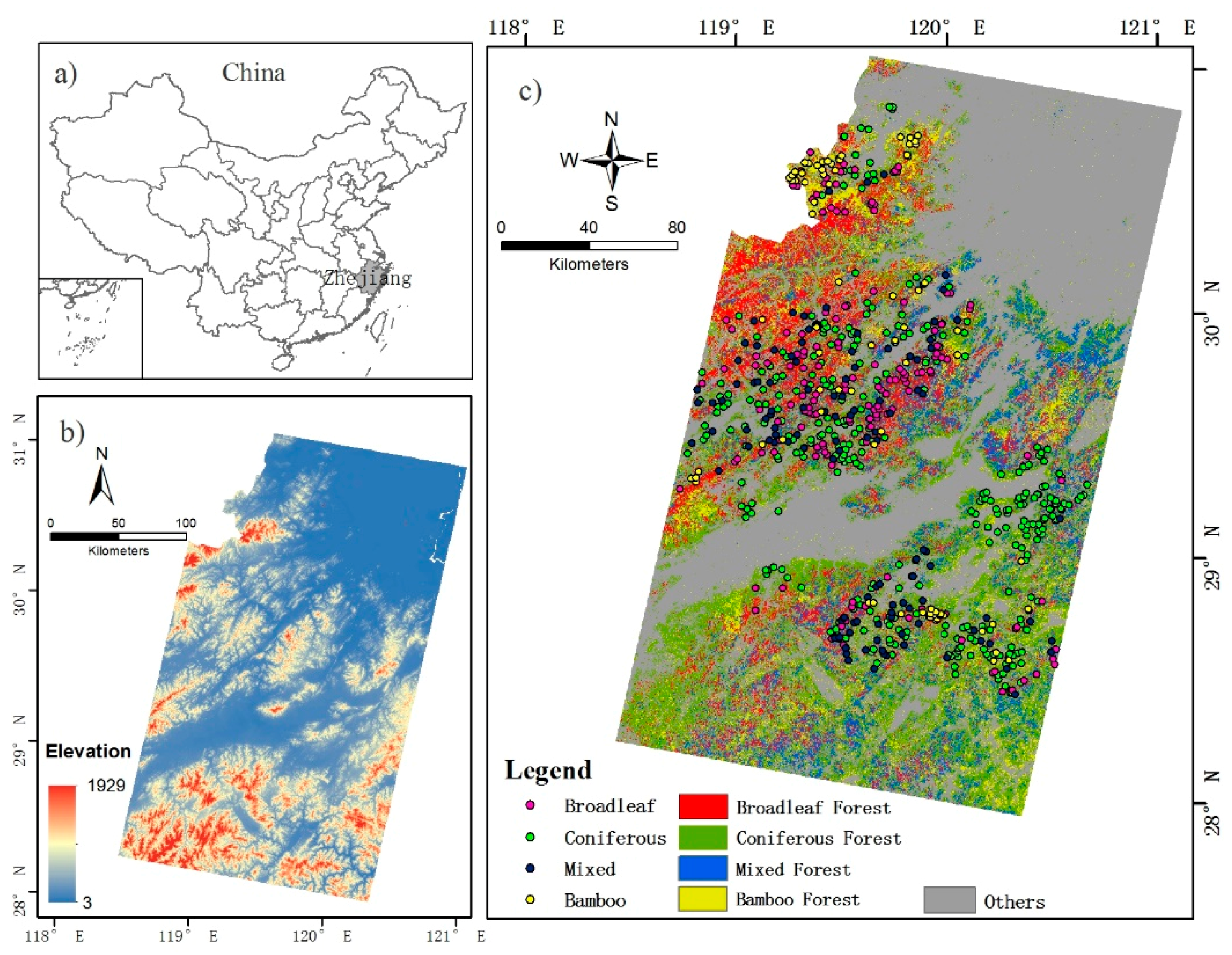
2. Study Area
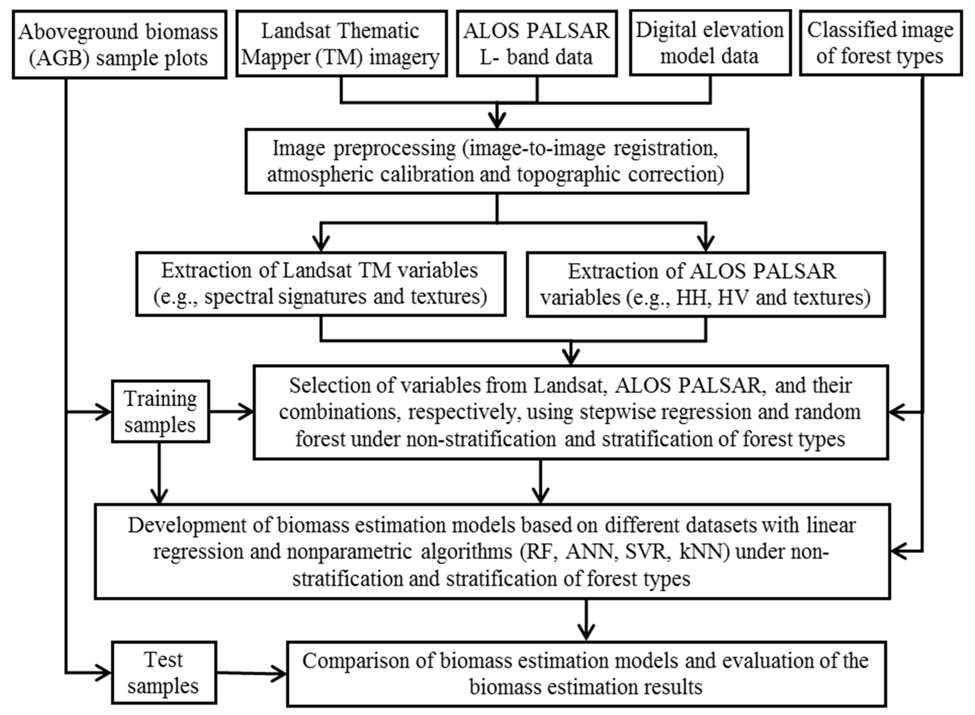
3. Materials and Methods
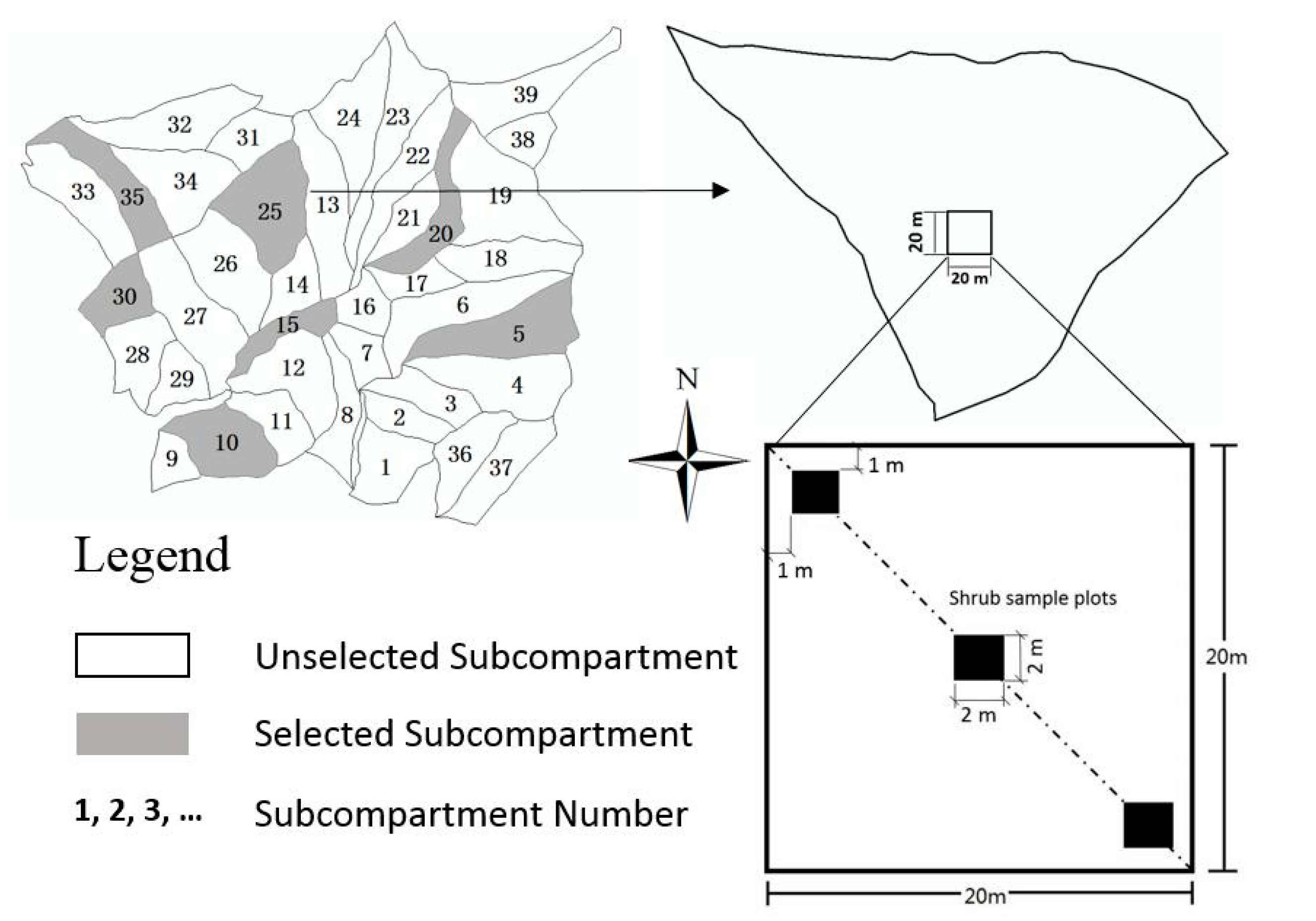
3.1. Data Collection and Preprocessing
3.2. Extraction and Selection of Variables from Landsat TM and ALOS PALSAR Data
3.3. Biomass Modeling Algorithms
3.4. AGB Modeling Based on Different Scenarios
3.5. Evaluation of AGB Estimates
4. Results
4.1. Comparative Analysis of AGB Modeling Results under Non-Stratification Scenarios
4.2. Comparative Analysis of AGB Modeling Results Based on Stratification of Forest Types
5. Discussion
5.1. Selection of Suitable Variables for AGB Modeling
5.2. Selection of Modeling Algorithms
5.3. Potential Solutions to Improve AGB Estimation
6. Conclusions
Acknowledgments
Author Contributions
Conflicts of Interest
References
- Zhu, J.; Huang, Z.; Sun, H.; Wang, G. Mapping forest ecosystem biomass density for Xiangjiang River Basin by combining plot and remote sensing data and comparing spatial extrapolation methods. Remote Sens. 2017, 9, 241. [Google Scholar] [CrossRef]
- Lu, D.; Chen, Q.; Wang, G.; Liu, L.; Li, G.; Moran, E. A survey of remote sensing-based aboveground biomass estimation methods in forest ecosystems. Int. J. Digit. Earth 2016, 9, 63–105. [Google Scholar] [CrossRef]
- Zhao, P.; Lu, D.; Wang, G.; Wu, C.; Huang, Y.; Yu, S. Examining spectral reflectance saturation in landsat imagery and corresponding solutions to improve forest aboveground biomass estimation. Remote Sens. 2016, 8, 469. [Google Scholar] [CrossRef]
- Lu, D. Aboveground biomass estimation using Landsat TM data in the Brazilian Amazon. Int. J. Remote Sens. 2005, 26, 2509–2525. [Google Scholar] [CrossRef]
- Lu, D.; Batistella, M. Exploring TM image texture and its relationships with biomass estimation in Rondônia, Brazilian Amazon. Acta Amaz. 2005, 35, 249–257. [Google Scholar] [CrossRef]
- Zhao, P.; Lu, D.; Wang, G.; Liu, L.; Li, D.; Zhu, J.; Yu, S. Forest aboveground biomass estimation in Zhejiang Province using the integration of Landsat TM and ALOS PALSAR data. Int. J. Appl. Earth Obs. Geoinf. 2016, 53, 1–15. [Google Scholar] [CrossRef]
- Breiman, L. Random forests. Mach. Learn. 2001, 45, 5–32. [Google Scholar] [CrossRef]
- Cutler, A.; Cutler, D.R.; Stevens, J.R. Random forests. In Ensemble Machine Learning: Methods and Applications; Springer: New York, NY, USA, 2012; pp. 157–175. ISBN 9781441993267. [Google Scholar]
- Feng, Y.; Lu, D.; Chen, Q.; Keller, M.; Moran, E.; dos-Santos, M.N.; Bolfe, E.L.; Batistella, M. Examining effective use of data sources and modeling algorithms for improving biomass estimation in a moist tropical forest of the Brazilian Amazon. Int. J. Digit. Earth 2017, 10, 996–1016. [Google Scholar] [CrossRef]
- Rodriguez-Galiano, V.F.; Ghimire, B.; Rogan, J.; Chica-Olmo, M.; Rigol-Sanchez, J.P. An assessment of the effectiveness of a random forest classifier for land-cover classification. ISPRS J. Photogramm. Remote Sens. 2012, 67, 93–104. [Google Scholar] [CrossRef]
- Fleming, A.L.; Wang, G.; McRoberts, R.E. Comparison of methods toward multi-scale forest carbon mapping and spatial uncertainty analysis: Combining national forest inventory plot data and landsat TM images. Eur. J. For. Res. 2015, 134, 125–137. [Google Scholar] [CrossRef]
- Chen, Q. Modeling aboveground tree woody biomass using national-scale allometric methods and airborne lidar. ISPRS J. Photogramm. Remote Sens. 2015, 106, 95–106. [Google Scholar] [CrossRef]
- Foody, G.M.; Cutler, M.E.; McMorrow, J.; Pelz, D.; Tangki, H.; Boyd, D.S.; Douglas, I. Mapping the biomass of Bornean tropical rain forest from remotely sensed data. Glob. Ecol. Biogeogr. 2001, 10, 379–387. [Google Scholar] [CrossRef]
- Reese, H.; Nilsson, M.; Sandström, P.; Olsson, H. Applications using estimates of forest parameters derived from satellite and forest inventory data. Comput. Electron. Agric. 2002, 37, 37–55. [Google Scholar] [CrossRef]
- Breidenbach, J.; Næsset, E.; Gobakken, T. Improving k-nearest neighbor predictions in forest inventories by combining high and low density airborne laser scanning data. Remote Sens. Environ. 2012, 117, 358–365. [Google Scholar] [CrossRef]
- McRoberts, R.E.; Chen, Q.; Domke, G.M.; Næsset, E.; Gobakken, T.; Chirici, G.; Mura, M. Optimizing nearest neighbour configurations for airborne laser scanning-assisted estimation of forest volume and biomass. Forestry 2017, 90, 99–111. [Google Scholar] [CrossRef]
- Saatchi, S.; Malhi, Y.; Zutta, B.; Buermann, W.; Anderson, L.O.; Araujo, A.M.; Phillips, O.L.; Peacock, J.; ter Steege, H.; Lopez Gonzalez, G.; et al. Mapping landscape scale variations of forest structure, biomass, and productivity in Amazonia. Biogeosci. Discuss. 2009, 6, 5461–5505. [Google Scholar] [CrossRef]
- Lek, S.; Guégan, J.F. Artificial neural networks as a tool in ecological modelling, an introduction. Ecol. Model. 1999, 120, 65–73. [Google Scholar] [CrossRef]
- Wang, S.; Guan, D. Remote sensing method of forest biomass estimation by artificial neural network models. Ecol. Environ. 2007, 16, 108–111. [Google Scholar] [CrossRef]
- Hame, T.; Salli, A.; Andersson, K.; Lohi, A. A new methodology for the estimation of biomass of coniferdominated boreal forest using NOAA AVHRR data. Int. J. Remote Sens. 1997, 18, 3211–3243. [Google Scholar] [CrossRef]
- Gleason, C.J.; Im, J. Forest biomass estimation from airborne LiDAR data using machine learning approaches. Remote Sens. Environ. 2012, 125, 80–91. [Google Scholar] [CrossRef]
- Li, M.; Im, J.; Quackenbush, L.J.; Liu, T. Forest biomass and carbon stock quantification using airborne LiDAR data: A case study over Huntington Wildlife Forest in the Adirondack Park. IEEE J. Sel. Top. Appl. Earth Obs. Remote Sens. 2014, 7, 3143–3156. [Google Scholar] [CrossRef]
- Kim, Y.H.; Im, J.; Ha, H.K.; Choi, J.K.; Ha, S. Machine learning approaches to coastal water quality monitoring using GOCI satellite data. Gisci. Remote Sens. 2014, 51, 158–174. [Google Scholar] [CrossRef]
- Zhang, J.; Huang, S.; Hogg, E.H.; Lieffers, V.; Qin, Y.; He, F. Estimating spatial variation in Alberta forest biomass from a combination of forest inventory and remote sensing data. Biogeosciences 2014, 11, 2793–2808. [Google Scholar] [CrossRef]
- Belgiu, M.; Drăgu, L. Random forest in remote sensing: A review of applications and future directions. ISPRS J. Photogramm. Remote Sens. 2016, 114, 24–31. [Google Scholar] [CrossRef]
- Houghton, R.A.; Butman, D.; Bunn, A.G.; Krankina, O.N.; Schlesinger, P.; Stone, T.A. Mapping Russian forest biomass with data from satellites and forest inventories. Environ. Res. Lett. 2007, 2, 45032–45037. [Google Scholar] [CrossRef]
- Ahmed, O.S.; Franklin, S.E.; Wulder, M.A.; White, J.C. Characterizing stand-level forest canopy cover and height using Landsat time series, samples of airborne LiDAR, and the Random Forest algorithm. ISPRS J. Photogramm. Remote Sens. 2015, 101, 89–101. [Google Scholar] [CrossRef]
- Baccini, A.; Friedl, M.A.; Woodcock, C.E.; Warbington, R. Forest biomass estimation over regional scales using multisource data. Geophys. Res. Lett. 2004, 31, 399–420. [Google Scholar] [CrossRef]
- Chirici, G.; Barbati, A.; Corona, P.; Marchetti, M.; Travaglini, D.; Maselli, F.; Bertini, R. Non-parametric and parametric methods using satellite images for estimating growing stock volume in alpine and Mediterranean forest ecosystems. Remote Sens. Environ. 2008, 112, 2686–2700. [Google Scholar] [CrossRef]
- Holmström, H.; Fransson, J.E.S. Combining remotely sensed optical and radar data in kNN-estimation of forest variables. For. Sci. 2003, 49, 409–418. [Google Scholar] [CrossRef]
- Katila, M.; Tomppo, E. Stratification by ancillary data in multisource forest inventories employing k-nearest-neighbour estimation. Can. J. For. Res. 2002, 32, 1548–1561. [Google Scholar] [CrossRef]
- McRoberts, R.E.; Magnussen, S.; Tomppo, E.O.; Chirici, G. Parametric, bootstrap, and jackknife variance estimators for the k-Nearest Neighbors technique with illustrations using forest inventory and satellite image data. Remote Sens. Environ. 2011, 115, 3165–3174. [Google Scholar] [CrossRef]
- McRoberts, R.E.; Næsset, E.; Gobakken, T. Optimizing the k-Nearest neighbors technique for estimating forest aboveground biomass using airborne laser scanning data. Remote Sens. Environ. 2015, 163, 13–22. [Google Scholar] [CrossRef]
- Tomppo, E.; Halme, M. Using coarse scale forest variables as ancillary information and weighting of variables in k-NN estimation: A genetic algorithm approach. Remote Sens. Environ. 2004, 92, 1–20. [Google Scholar] [CrossRef]
- Tomppo, E.; Olsson, H.; Ståhl, G.; Nilsson, M.; Hagner, O.; Katila, M. Combining national forest inventory field plots and remote sensing data for forest databases. Remote Sens. Environ. 2008, 112, 1982–1999. [Google Scholar] [CrossRef]
- Ahern, F.J.; Erdle, T.; Maclean, D.A.; Kneppeck, I.D. A quantitative relationship between forest growth rates and thematic mapper reflectance measurements. Int. J. Remote Sens. 1991, 12, 387–400. [Google Scholar] [CrossRef]
- McRoberts, R.E. Estimating forest attribute parameters for small areas using nearest neighbors techniques. For. Ecol. Manag. 2012, 272, 3–12. [Google Scholar] [CrossRef]
- Cherkassky, V.; Ma, Y. Practical selection of SVM parameters and noise estimation for SVM regression. Neural Netw. 2004, 17, 113–126. [Google Scholar] [CrossRef]
- Chander, G.; Markham, B.L.; Helder, D.L. Summary of current radiometric calibration coefficients for Landsat MSS, TM, ETM+, and EO-1 ALI sensors. Remote Sens. Environ. 2009, 113, 893–903. [Google Scholar] [CrossRef]
- Chávez, P.S.J. Image-based atmospheric corrections—Revisited and improved. Photogramm. Eng. Remote Sens. 1996, 62, 1025–1036. [Google Scholar]
- Reese, H.; Olsson, H. C-correction of optical satellite data over alpine vegetation areas: A comparison of sampling strategies for determining the empirical c-parameter. Remote Sens. Environ. 2011, 115, 1387–1400. [Google Scholar] [CrossRef]
- Lee, J.S.; Jurkevich, I.; Dewaele, P.; Wambacq, P.; Oosterlinck, A. Speckle filtering of synthetic aperture radar images: A review. Remote Sens. Rev. 1994, 8, 313–340. [Google Scholar] [CrossRef]
- Qian, Y.; Yi, L.; Zhang, C.; Yu, S.; Shen, L.; Peng, D.; Zheng, C. Biomass and Carbon Storage of Public Service Forests in the Central Area of Zhejiang Province. Sci. Silvae Sin. 2013, 49, 17–23. [Google Scholar] [CrossRef]
- Yuan, W.; Jiang, B.; Ge, Y.; Zhu, J.; Shen, A. Study on biomass models of important commonwealth forests for Zhejiang Province. J. Zhejiang For. Sci. Technol. 2009, 29, 1–5. [Google Scholar]
- Lu, D.; Mausel, P.; Brondízio, E.; Moran, E. Relationships between forest stand parameters and Landsat TM spectral responses in the Brazilian Amazon Basin. For. Ecol. Manag. 2004, 198, 149–167. [Google Scholar] [CrossRef]
- Koukal, T.; Suppan, F.; Schneider, W. The impact of relative radiometric calibration on the accuracy of kNN-predictions of forest attributes. Remote Sens. Environ. 2007, 110, 431–437. [Google Scholar] [CrossRef]
- Avitabile, V.; Baccini, A.; Friedl, M.A.; Schmullius, C. Capabilities and limitations of Landsat and land cover data for aboveground woody biomass estimation of Uganda. Remote Sens. Environ. 2012, 117, 366–380. [Google Scholar] [CrossRef]
- Baccini, A.; Laporte, N.T.; Goetz, S.J.; Sun, M.; Dong, H. A first map of tropical Africa’s above-ground biomass derived from satellite imagery. Environ. Res. Lett. 2008, 3, 45011. [Google Scholar] [CrossRef]
- Tanase, M.A.; Panciera, R.; Lowell, K.; Tian, S.; Hacker, J.M.; Walker, J.P. Airborne multi-temporal L-band polarimetric SAR data for biomass estimation in semi-arid forests. Remote Sens. Environ. 2014, 145, 93–104. [Google Scholar] [CrossRef]
- Vincenzi, S.; Zucchetta, M.; Franzoi, P.; Pellizzato, M.; Pranovi, F.; De Leo, G.A.; Torricelli, P. Application of a Random Forest algorithm to predict spatial distribution of the potential yield of Ruditapes philippinarum in the Venice lagoon, Italy. Ecol. Model. 2011, 222, 1471–1478. [Google Scholar] [CrossRef]
- Pflugmacher, D.; Cohen, W.B.; Kennedy, R.E.; Yang, Z. Using Landsat-derived disturbance and recovery history and lidar to map forest biomass dynamics. Remote Sens. Environ. 2014, 151, 124–137. [Google Scholar] [CrossRef]
- Ismail, R.; Mutanga, O.; Kumar, L. Modeling the Potential Distribution of Pine Forests Susceptible to Sirex Noctilio Infestations in Mpumalanga, South Africa. Trans. GIS 2010, 14, 709–726. [Google Scholar] [CrossRef]
- McInerney, D.O.; Suarez-Minguez, J.; Valbuena, R.; Nieuwenhuis, M. Forest canopy height retrieval using LiDAR data, medium-resolution satellite imagery and kNN estimation in Aberfoyle, Scotland. Forestry 2010, 83, 195–206. [Google Scholar] [CrossRef]
- Lu, D.; Batistella, M.; Moran, E. Satellite estimation of aboveground biomass and impacts of forest stand structure. Photogramm. Eng. Remote Sens. 2005, 71, 967–974. [Google Scholar] [CrossRef]
- Chrysafis, I.; Mallinis, G.; Gitas, I.; Tsakiri-Strati, M. Estimating Mediterranean forest parameters using multi seasonal Landsat 8 OLI imagery and an ensemble learning method. Remote Sens. Environ. 2017, 199, 154–166. [Google Scholar] [CrossRef]
- Hame, T.; Rauste, Y.; Antropov, O.; Ahola, H.A.; Kilpi, J. Improved mapping of tropical forests with optical and SAR imagery, part II: Above ground biomass estimation. IEEE J. Sel. Top. Appl. Earth Obs. Remote Sens. 2013, 6, 92–101. [Google Scholar] [CrossRef]
- Li, G.; Lu, D.; Moran, E.; Dutra, L.; Batistella, M. A comparative analysis of ALOS PALSAR L-band and RADARSAT-2 C-band data for land-cover classification in a tropical moist region. ISPRS J. Photogramm. Remote Sens. 2012, 70, 26–38. [Google Scholar] [CrossRef]
- Li, G.; Lu, D.; Moran, E.; Sant’Anna, S.J.S. Comparative analysis of classification algorithms and multiple sensor data for land use/land cover classification in the Brazilian Amazon. J. Appl. Remote Sens. 2012, 6, 61706. [Google Scholar] [CrossRef]


| Dataset | Description |
|---|---|
| Landsat 5 TM imagery | Two scenes of TM images (Path/row: 119/39 and 119/40) with a 30-m spatial resolution were acquired on 24 May 2010. Six spectral bands were used to develop the forest classification map [3] and for AGB estimation in this research |
| ALOS PALSAR L-band | The FBD (fine beam double polarization, HH/HV) L-band 1.5 product with 25-m cell size was downloaded from the global mosaic data with a time interval of 1 year. This downloaded image was produced using the 2010 PALSAR images. The cell size of 25-m was resampled to a 30-m cell size during the PALSAR-to-TM image registration |
| ASTER GDEM data | Global digital elevation model (GDEM) data with a 30-m spatial resolution were downloaded from the United States Geological Survey website |
| Forest classification image | The forest types in this study area included pine and fir (coniferous forest), broadleaf forest, mixed forest, and bamboo. The forest distribution map was developed from a Landsat TM image using a hybrid approach [3] with an overall classification accuracy of 78%. Forest classes had user’s accuracy between 71 and 87% and producer’s accuracy between 72 and 87%. More details are provided in [3]. |
| Field measurements | A total of 664 sample plots covering coniferous, broadleaf, mixed, and bamboo forests were inventoried in 2010 and 2011 [3] |
| No. of Total Samples | AGB Range (Mg/ha) | Mean (Mg/ha) | Standard Deviation | No. of Training Samples | No. of Test Samples | |
|---|---|---|---|---|---|---|
| Stratification based on forest type | ||||||
| Coniferous | 329 | 32.1–180.1 | 101.7 | 31.8 | 230 | 99 |
| Broadleaf | 143 | 26.5–175.7 | 94.7 | 34.6 | 100 | 43 |
| Mixed | 117 | 41.6–180.7 | 105.0 | 32.2 | 82 | 35 |
| Bamboo | 75 | 25.7–123.9 | 61.2 | 18.4 | 53 | 22 |
| Non-stratification | 664 | 25.7–180.7 | 95.9 | 33.9 | 498 | 166 |
| Datasets | Models | R2 |
|---|---|---|
| Landsat TM | YTM = 111.058 − 24.186Tb7w3ME + 4.549Tb7w3CON + 23.233Tb4w5EN + 9.641Tb7w3COR + 9.132Tb3w3ME | 0.36 |
| ALOS PALSAR | YSAR = 44.761 + 13.553THVw5ME + 43.273THVw7DI − 44.889THVw3VA + 15.513THHw3COR − 35.278THHw7COR + 17.115THVw3CON − 4.315THHw9CON + 23.215THVw7VA | 0.19 |
| Combination | Ycomb = 179.760 − 23.772Tb7w3ME + 12.772Tb7w3VA + 51.012THVw7DI − 33.133THHw9COR + 12.233THHw3COR − 31.541Tb4w5HO + 8.998Tb2w5ME − 5.177THHw9CON + 2.989THHw5CON − 16.234THVw3VA | 0.41 |
| Datasets | The Identified Variables from Different Remote Sensing Data | R2 |
|---|---|---|
| Landsat TM | Sb7, Tb7w3ME, Tb3w5SM, Tb4w5HO, Tb7w5DI, Tb3w7VA, Tb7w7EN, Tb5w9ME | 0.87 |
| ALOS PALSAR | THHw3ME, THHw7ME, THHw5HO, THHw9SM, THHw9VA, HV, THVw7ME, THVw5HO, THVw9CON, THVw9EN, THVw9VA | 0.62 |
| Combination | Sb7, HH, THHw5ME, HV, THVw7ME, THVw7CON, THVw9EN | 0.60 |
| Data | Models | Mean | Std Dev | Minimum | Maximum | Data Range |
|---|---|---|---|---|---|---|
| Landsat TM | RF | 93.0 | 22.9 | 42.0 | 148.7 | 106.7 |
| ANN | 88.4 | 26.6 | 19.1 | 187.1 | 168.0 | |
| SVR | 88.3 | 22.2 | 19.3 | 149.0 | 129.7 | |
| kNN | 88.8 | 26.9 | 32.9 | 164.7 | 131.8 | |
| LR | 90.6 | 26.2 | 1.7 | 180.0 | 178.3 | |
| ALOS PALSAR | RF | 92.4 | 15.2 | 39.8 | 153.8 | 114.0 |
| ANN | 91.8 | 17.0 | 1.6 | 150.5 | 148.9 | |
| SVR | 91.5 | 11.3 | 19.6 | 122.1 | 102.5 | |
| kNN | 93.7 | 14.7 | 55.8 | 127.1 | 71.3 | |
| LR | 92.1 | 18.4 | 1.5 | 135.5 | 134.0 | |
| Combination | RF | 93.0 | 22.9 | 41.9 | 148.8 | 106.9 |
| ANN | 90.2 | 26.3 | 0.7 | 181.3 | 180.6 | |
| SVR | 86.6 | 24.5 | 0.7 | 176.1 | 175.4 | |
| kNN | 92.0 | 16.6 | 43.2 | 137.7 | 94.5 | |
| LR | 89.8 | 29.7 | 1.6 | 177.8 | 176.2 | |
| Sample plots | Statistics | 95.9 | 33.9 | 25.7 | 180.7 | 155.0 |
| Datasets | Landsat TM | ALOS PALSAR | Combination | ||||
|---|---|---|---|---|---|---|---|
| Algorithms | RMSE | RMSEr | RMSE | RMSEr | RMSE | RMSEr | |
| RF | 28.4 | 29.5 | 33.2 | 34.5 | 30.3 | 31.5 | |
| ANN | 27.7 | 28.8 | 30.3 | 31.5 | 27.6 | 28.7 | |
| SVR | 28.2 | 29.3 | 32.1 | 33.4 | 28.2 | 29.3 | |
| kNN | 28.3 | 29.4 | 33.7 | 35.0 | 30.8 | 32.0 | |
| LR | 29.3 | 30.5 | 32.9 | 34.2 | 27.7 | 28.8 | |
| Data | Model | RMSE (Mg/ha) | ||||||||
| Overall | Forest Type | AGB Ranges (Mg/ha) | ||||||||
| MXF | BLF | CFF | BBF | <40 | 40–120 | 120–160 | >160 | |||
| Landsat TM | RF | 28.4 | 32.0 | 26.2 | 28.6 | 24.4 | 34.6 | 23.2 | 35.9 | 53.6 |
| ANN | 27.7 | 30.0 | 26.2 | 28.6 | 25.0 | 37.4 | 25.5 | 29.1 | 50.2 | |
| SVR | 28.2 | 31.9 | 25.4 | 28.7 | 23.9 | 36.7 | 24.5 | 30.5 | 57.5 | |
| kNN | 28.3 | 32.6 | 26.5 | 28.5 | 22.0 | 29.7 | 24.7 | 34.7 | 61.0 | |
| LR | 29.3 | 32.6 | 24.4 | 28.7 | 21.3 | 35.0 | 22.4 | 34.2 | 61.0 | |
| ALOS PALSAR | RF | 33.2 | 36.8 | 29.5 | 33.8 | 28.5 | 42.5 | 27.4 | 36.9 | 74.6 |
| ANN | 30.3 | 36.0 | 26.4 | 30.9 | 31.1 | 45.2 | 25.2 | 35.4 | 67.8 | |
| SVR | 32.1 | 35.4 | 28.2 | 31.9 | 34.7 | 50.6 | 24.7 | 32.2 | 73.6 | |
| kNN | 33.7 | 39.2 | 31.6 | 32.9 | 32.8 | 46.0 | 26.3 | 40.6 | 78.6 | |
| LR | 32.9 | 37.0 | 31.0 | 32.4 | 32.0 | 47.5 | 27.3 | 37.1 | 70.3 | |
| Comb. | RF | 30.3 | 35.6 | 26.1 | 30.4 | 28.5 | 39.3 | 23.5 | 37.8 | 68.3 |
| ANN | 27.6 | 31.7 | 24.0 | 28.2 | 23.4 | 35.5 | 23.7 | 31.6 | 53.6 | |
| SVR | 28.2 | 33.3 | 23.9 | 29.0 | 21.6 | 34.0 | 23.9 | 32.7 | 56.3 | |
| kNN | 30.8 | 35.2 | 28.7 | 30.6 | 28.1 | 35.9 | 25.3 | 36.1 | 68.3 | |
| LR | 27.7 | 34.4 | 24.9 | 28.2 | 20.9 | 35.7 | 22.9 | 32.4 | 58.6 | |
| Data | Model | RMSEr (%) | ||||||||
| Overall | Forest Type | AGB Ranges (Mg/ha) | ||||||||
| MXF | BLF | CFF | BBF | <40 | 40–120 | 120–160 | >160 | |||
| Landsat TM | RF | 29.5 | 30.4 | 29.3 | 27.4 | 47.7 | 95.7 | 27.8 | 26.3 | 31.3 |
| ANN | 28.8 | 28.5 | 29.3 | 27.4 | 48.9 | 103.4 | 30.5 | 21.3 | 29.3 | |
| SVR | 29.3 | 30.3 | 28.4 | 27.5 | 46.8 | 101.5 | 29.3 | 22.3 | 33.6 | |
| kNN | 29.4 | 31.0 | 29.7 | 27.3 | 43.0 | 82.2 | 29.6 | 25.4 | 35.6 | |
| LR | 30.5 | 31.0 | 27.3 | 27.5 | 41.7 | 96.8 | 26.8 | 25.0 | 35.6 | |
| ALOS PALSAR | RF | 34.5 | 34.9 | 33.0 | 32.4 | 55.8 | 117.6 | 32.8 | 27.0 | 43.6 |
| ANN | 31.5 | 34.2 | 29.6 | 29.6 | 60.8 | 125.0 | 30.2 | 25.9 | 39.6 | |
| SVR | 33.4 | 33.6 | 31.6 | 30.6 | 67.9 | 140.0 | 29.6 | 23.6 | 43.0 | |
| kNN | 35.0 | 37.2 | 35.4 | 31.5 | 64.2 | 127.2 | 31.5 | 29.7 | 45.9 | |
| LR | 34.2 | 35.1 | 34.7 | 31.1 | 62.6 | 131.4 | 32.7 | 27.2 | 41.1 | |
| Comb. | RF | 31.5 | 33.8 | 29.2 | 29.1 | 55.8 | 108.7 | 28.1 | 27.7 | 39.9 |
| ANN | 28.7 | 30.1 | 26.9 | 27.0 | 45.8 | 98.2 | 28.4 | 23.1 | 31.3 | |
| SVR | 29.3 | 31.6 | 26.8 | 27.8 | 42.3 | 94.0 | 28.6 | 23.9 | 32.9 | |
| kNN | 32.0 | 33.4 | 32.1 | 29.3 | 55.0 | 99.3 | 30.3 | 26.4 | 39.9 | |
| LR | 28.8 | 32.7 | 27.9 | 27.0 | 40.9 | 98.7 | 27.4 | 23.7 | 34.2 | |
| Data | Linear Regression Models for Different Forest Types | |||
|---|---|---|---|---|
| MXF | BLF | CFF | BBF | |
| Landsat TM | YTM = 71.008 + 40.317Tb3w9COR − 10.625Tb7w9ME + 52.797Tb2w3CON − 206.413Tb4w5HO + 109.316Tb5w5HO + 260.741Tb4w3SM + 104.65Tb3w9HO − 6.329Tb5w3ME | YTM = 177.747 − 0.165Sb7 + 0.151Sb3 − 28.648Tb5w5COR − 20.974Tb2w9CON + 1.282Tb4w3VA | YTM = 183.858 − 0.021Sb5 − 118.949Tb5w5SM − 9.12Tb7w3ME | YTM = 96.657 + 23.498Tb2w7COR − 8.597Tb7w9ME |
| ALOS PALSAR | YSAR=174.082 − 11.082THHw9ME | YSAR = 151.113 − 70.931THHw7COR − 144.26THHw7SM − 55.692THVw9CON | YSAR = 175.648 + 20.049THHw3COR− 41.359THHw7COR − 150.38THVw7HO+ 13.14THHw5ME − 38.094THHw9DI + 19.933THVw5COR | YSAR = 120.636 + 63.802THVw7CON − 38.269THHw9EN + 19.958THHw5COR − 39.861THVw3VA + 0.009HV − 164.441THHw9SM |
| Comb. | Ycomb=176.174 + 43.325Tb3w9COR − 11.337Tb7w9ME + 68.823Tb2w3CON − 205.811Tb4w5HO + 116.538Tb5w5HO + 315.581Tb4w3SM − 8.284THHw3ME − 52.339Tb3w7VA − 2.713Tb4w3ME + 36.675THHw3HO | Ycomb = 245.956 − 0.155Sb7 − 74.642THHw7HO − 50.144THHw9COR + 0.123Sb3 | Ycomb = 179.245 − 0.044Sb5 + 23.818THHw3COR − 52.009Tb5w5HO + 11.293THVw5ME − 42.93THVw7COR + 25.813THVw5COR + 18.357Tb7w7COR + 7.282THHw3CON − 31.22THHw5EN + 19.111THHw3EN | Ycomb = 199.125 + 123.557THVw7CON − 41.769THHw9EN + 25.32Tb2w7COR + 27.018THHw5COR − 40.484Tb4w3HO − 125.836THHw9HO + 35.594Tb7w3SM + 0.006Sb4 − 105.66THVw7DI |
| Data | The Selected Variables for Different Forest Types Using the RF Approach | |||
|---|---|---|---|---|
| MXF | BLF | CFF | BBF | |
| Landsat TM | Tb3w7COR, Tb3w9COR, Tb4w9ME, Tb5w3ME, | Tb4w9COR, Tb5w5VA, Tb5w5COR, Tb5w9ME, Tb7w3ME | Sb3, Sb5, Tb3w9VA, Tb4w7DI, Tb5w5ME, Tb5w5DI, Tb5w7EN, Tb5w7VA, Tb7w3ME, Tb5w7ME,Tb7w9SM | Tb2w7VA, Tb3w7COR, Tb3w9COR, Tb4w3ME, Tb4w9ME, Tb5w3ME, Tb5w9ME |
| ALOS PALSAR | THHw9CON, THHw7HO, THVw3SM, THVw5SM, THVw7VA,THVw7HO THVw9SM | HH, THHw5ME, THHw7CON, THHw7COR, THHw9SM, THVw7CON, THVw9EN | HH, THHw3COR, THHw3VA, THHw5DI, THHw7ME, THHw9CON, THHw9VA, THHw9HO, THHw9SM, THVw3SM, THVw5ME | HV, THHw3VA, THHw5ME, THHw5EN, THHw9EN, THVw7HO, THVw9VA, THVw9SM |
| Comb. | Sb5,Tb2w7VA, Tb3w7COR, Tb3w9COR, Tb4w3ME, Tb4w9ME, Tb5w5ME, Tb6w7ME | Sb5, Tb5w9ME, Tb5w3ME, THHw7COR, THVw7HO | Sb3, Sb6, Tb5w3ME, Tb4w7DI, Tb6w5ME, Tb6w5HO, Tb6w5COR, THHw3COR, THHw3VA, THHw7ME | Tb4w3ME, Tb4w7VA, Tb5w5ME, HV, THHw3ME, THVw7HO |
| Data | Model | RMSE (Mg/ha) | ||||||||
| Overall | Forest Type | AGB Range (Mg/ha) | ||||||||
| MXF | BLF | CFF | BBF | <40 | 40–120 | 120–160 | >160 | |||
| Landsat TM | RF | 26.8 | 28.8 | 24.5 | 27.3 | 20.4 | 34.5 | 23.0 | 28.8 | 50.4 |
| ANN | 25.5 | 28.8 | 24.2 | 26.4 | 19.9 | 31.6 | 21.6 | 29.1 | 50.4 | |
| SVR | 25.8 | 28.4 | 25.1 | 26.9 | 20.8 | 35.4 | 24.0 | 28.7 | 51.5 | |
| kNN | 28.0 | 28.9 | 26.5 | 29.1 | 21.9 | 28.1 | 24.5 | 33.7 | 53.4 | |
| LR | 27.4 | 28.7 | 25.4 | 26.7 | 21.4 | 35.4 | 22.6 | 33.6 | 53.9 | |
| ALOS PALSAR | RF | 30.2 | 30.7 | 29.5 | 30.8 | 24.6 | 39.3 | 25.1 | 36.5 | 63.8 |
| ANN | 28.0 | 28.1 | 29.3 | 27.6 | 21.0 | 41.1 | 23.6 | 34.1 | 60.0 | |
| SVR | 29.1 | 29.8 | 30.3 | 28.8 | 22.5 | 46.9 | 23.7 | 31.8 | 60.1 | |
| kNN | 29.9 | 31.9 | 30.6 | 29.0 | 23.7 | 47.1 | 24.6 | 37.5 | 64.3 | |
| LR | 29.8 | 31.7 | 31.1 | 29.5 | 22.1 | 48.5 | 25.4 | 36.6 | 58.5 | |
| Comb. | RF | 26.1 | 27.1 | 24.8 | 28.5 | 23.4 | 35.3 | 23.0 | 33.3 | 62.8 |
| ANN | 24.7 | 26.8 | 23.5 | 25.9 | 19.1 | 30.4 | 21.6 | 25.1 | 52.0 | |
| SVR | 25.7 | 27.8 | 24.4 | 27.1 | 20.3 | 32.1 | 23.2 | 31.9 | 49.6 | |
| kNN | 26.5 | 27.3 | 25.2 | 27.7 | 20.7 | 33.9 | 34.1 | 33.5 | 59.4 | |
| LR | 26.4 | 27.9 | 25.4 | 26.1 | 20.6 | 34.3 | 22.1 | 31.0 | 41.5 | |
| Data | Model | RMSEr (%) | ||||||||
| Overall | Forest Type | AGB Range (Mg/ha) | ||||||||
| MXF | BLF | CFF | BBF | <40 | 40–120 | 120–160 | >160 | |||
| Landsat TM | RF | 27.9 | 27.4 | 27.4 | 26.2 | 39.9 | 97.1 | 27.7 | 21.2 | 29.9 |
| ANN | 26.5 | 27.4 | 27.1 | 25.3 | 38.9 | 88.9 | 26.0 | 21.3 | 29.9 | |
| SVR | 26.8 | 27.0 | 28.1 | 25.8 | 40.7 | 99.6 | 28.9 | 21.1 | 30.6 | |
| kNN | 29.1 | 27.4 | 29.7 | 27.9 | 42.8 | 79.1 | 29.5 | 24.8 | 31.8 | |
| LR | 28.4 | 27.3 | 28.4 | 25.6 | 41.9 | 99.6 | 27.2 | 24.7 | 32.1 | |
| ALOS PALSAR | RF | 31.4 | 29.2 | 33.0 | 29.5 | 48.1 | 110.5 | 30.2 | 26.8 | 37.9 |
| ANN | 29.1 | 26.7 | 32.8 | 26.5 | 41.1 | 115.6 | 28.4 | 25.1 | 35.7 | |
| SVR | 30.2 | 28.3 | 33.9 | 27.6 | 44.0 | 131.9 | 28.5 | 23.4 | 35.7 | |
| kNN | 31.1 | 30.3 | 34.3 | 27.8 | 46.4 | 132.5 | 29.6 | 27.6 | 38.2 | |
| LR | 31.0 | 30.1 | 34.8 | 28.3 | 43.2 | 136.4 | 30.6 | 26.9 | 34.8 | |
| Comb. | RF | 27.1 | 25.7 | 27.8 | 27.3 | 45.8 | 99.3 | 27.7 | 24.5 | 37.3 |
| ANN | 25.7 | 25.5 | 26.3 | 24.8 | 37.4 | 85.5 | 26.0 | 18.4 | 30.9 | |
| SVR | 26.7 | 26.4 | 27.3 | 26.0 | 39.7 | 90.3 | 27.9 | 23.4 | 29.4 | |
| kNN | 27.5 | 25.9 | 28.2 | 26.5 | 40.5 | 95.4 | 29.0 | 24.7 | 35.3 | |
| LR | 27.4 | 26.5 | 28.4 | 25.0 | 40.3 | 96.5 | 26.6 | 22.8 | 24.7 | |
© 2018 by the authors. Licensee MDPI, Basel, Switzerland. This article is an open access article distributed under the terms and conditions of the Creative Commons Attribution (CC BY) license (http://creativecommons.org/licenses/by/4.0/).
Share and Cite
Gao, Y.; Lu, D.; Li, G.; Wang, G.; Chen, Q.; Liu, L.; Li, D. Comparative Analysis of Modeling Algorithms for Forest Aboveground Biomass Estimation in a Subtropical Region. Remote Sens. 2018, 10, 627. https://doi.org/10.3390/rs10040627
Gao Y, Lu D, Li G, Wang G, Chen Q, Liu L, Li D. Comparative Analysis of Modeling Algorithms for Forest Aboveground Biomass Estimation in a Subtropical Region. Remote Sensing. 2018; 10(4):627. https://doi.org/10.3390/rs10040627
Chicago/Turabian StyleGao, Yukun, Dengsheng Lu, Guiying Li, Guangxing Wang, Qi Chen, Lijuan Liu, and Dengqiu Li. 2018. "Comparative Analysis of Modeling Algorithms for Forest Aboveground Biomass Estimation in a Subtropical Region" Remote Sensing 10, no. 4: 627. https://doi.org/10.3390/rs10040627
APA StyleGao, Y., Lu, D., Li, G., Wang, G., Chen, Q., Liu, L., & Li, D. (2018). Comparative Analysis of Modeling Algorithms for Forest Aboveground Biomass Estimation in a Subtropical Region. Remote Sensing, 10(4), 627. https://doi.org/10.3390/rs10040627