Hyperspectral Image Resolution Enhancement Approach Based on Local Adaptive Sparse Unmixing and Subpixel Calibration

Abstract

Unmixing based fusion aims at generating a high spectral-spatial resolution image (HSS) with the same surface features of the high spatial resolution multispectral image (MS) and low spatial resolution hyperspectral image (HS). In this paper, a new fusion method is proposed to improve the fusion performance by taking further advantage of the distribution characteristics of ground objects. First, we put forward a local adaptive sparse unmixing based fusion (LASUF) algorithm, in which the sparsity of the abundance matrices is appended as the constraint to the optimization fusion, considering the limited categories of ground objects in a specific range and the local correlation of their distribution. Then, to correct the possible original subpixel misregistrations or those introduced by the fusion procedures, a subpixel calibration method based on optimal matching adaptive morphology filtering (OM-AMF) is designed. Experiments on various datasets captured by different sensors demonstrate that the proposed fusion algorithm surpasses other typical fusion techniques in both spatial and spectral domains. The proposed method effectively preserves the spectral composition features of the isolated ground objects within a small area. In addition, the OM-AMF postprocessing is able to spatially correct the fusion results at a subpixel level and preserve the spectral features simultaneously.

1. Introduction

Along with the innovation of imaging spectroscopy, hyperspectral (HS) images can provide a spatial scene in hundreds of spectral channels. The high spectral resolution can reflect diagnostic spectrum characteristics of ground materials, and HS data have obvious superiority in aspects such as precision agriculture, anomaly detection, mineral exploration and terrain classification. Nevertheless, the spatial resolution of HS imagery is relatively low compared to panchromatic (PAN) imagery and multispectral (MS) imagery in order to maintain an acceptable signal-to-noise ratio (SNR), narrow the spectral bandwidth needed to increase instantaneous field of view (IFOV), while having high spatial resolution (small IFOV) system needed to broaden spectral channel. Due to the trade-off between spectral and spatial information quality, it is hard to directly get high spectral-spatial (HSS) resolution data, which are required in various applications. Performing algorithms from image processing perspective is a very feasible way to overcome this problem.

To obtain HSS data, plenty of resolution enhancement methods can be found in literature [1,2,3]. Under certain circumstances, auxiliary information can be hard to acquire, and single image super-resolution aims to reconstruct high spatial resolution data from low-resolution HS images. The basic approach through traditional interpolators was simple and fast, but it did not enhance the details. Various regularization-based methods were proposed to solve such an ill-posed problem including total variation regularization [4], sparse representation [5], and self-similarity grouping [6]. The introduction of regularization terms can preserve the edges and textures, so better performances were realized during the super-resolution process. Gu et al. [7] mapped abundance after unmixing on a high-resolution grid using spatial correlation to get resolution enhanced data. However, single image super-resolution mainly depends on priori and models, which are not universally applicable. With the development of a remote sensing platform carrying different sensors, multi sources are more available. Component substitution (CS) [8,9,10] relied on replacing components of MS data by panchromatic images. A multiresolution analysis (MRA) based approach injected spatial details obtained from multiscale decomposition of panchromatic images into MS data [11,12]. A combination of CS and MRA, named Hybrid, and a series of derivative algorithms were proposed to provide an appropriate balance between spatial and spectral preservation [13,14]. Pansharpening techniques achieved remarkable results due to information injection and were extended to HS and MS imagery fusion in the last few decades. Since both spatial and spectral information is contained in MS images, and the corresponding bands are highly correlated to HS images, image fusion has received extensive attention [15]. In this paper, we mainly discuss the HSS image generation utilizing HS and MS image fusion techniques.

From the literature, the first algorithm of merging HS and MS images was a wavelet-based method [16]. Both the images were transformed in wavelet space and then combined according to a fusion rule. Then, the contourlet transform compromising multi-scale and directional filters in its structure was developed [17]. Some researchers established the observation model between HS and MS images to estimate HSS data. Eismann [18,19,20] developed a maximum a posteriori (MAP) estimator incorporating with a stochastic mixing model (SMM), and minimized the objective function considering the underlying spectral characteristics and spatial position to get the optimal estimation. The Bayesian estimator [21,22,23,24,25] was another popular approach suited for the observation model. The spectral response function needed to be explored, and then the distribution of HS and MS data was estimated by the assumed priori distribution. The fusion model was processed via the posteriori distribution. The key step was the definition of the penalization term, and various estimators can be implemented: native Gaussian prior, sparse representation promoted prior, and vector total variation prior. Unmixing based fusion methods were proposed recently, in which the coupled nonnegative matrix factorization (CNMF) was the most famous one [26]. The theoretical foundation of CNMF was a linear spectral mixing model, and both low spatial resolution HS and high spatial resolution MS images were iteratively unmixed to eventually extract a high quality of endmembers and abundance maps. HSS imagery was then produced by endmember spectral of HS image and abundance map of MS image. Yokoya applied preprocessing and onboard cross-calibration into CNMF and solved the spectral range mismatch between real data [27]. Bendoumi added sub-image division to the original CNMF framework and simplified the solving process to get good fusion results [28]. In [29], spectral adjustment was used after CNMF to generate a simulated MS image and reduce the spectral distortion during simulation. High frequency information was extracted by a block based fusion phase. Compared with other fusion procedures, unmixing based methods attempted to approach physical reality more than mathematic approximation. However, the physical constraints of priori knowledge were almost neglected in the iterative solution of previous unmixing based methods.

In recent years, the sparsity of the HS images has been gradually regarded and taken advantage of in the resolution enhancement methods. By implementing an alternating direction method of multipliers (ADMM), Wycoff [30] transformed the optimization problem of integrating hyperspectral and visual color images into two Frobenius norm minimization problems utilizing coefficients matrix sparsity to improve the efficiency. However, the sparsity property of coefficients matrix was not further considered during the ADMM iterations, and fusion accuracy was not promoted markedly. In [31], mutual correlations between different HS channels were used to jointly sparse coefficient vectors, and dictionaries were created for each MS channel. Qi Wei [32] formed regularization priors and posteriori optimization to the joint nonnegative matrix factorization (NMF) problem, and the ADMM algorithm was used to alternately estimate the final abundance maps and endmember signatures. The authors [33] proposed a Generalization of Simultaneous Orthogonal Matching Pursuit (G-SOMP+) algorithm to learn a sparse code, and then the HSS image was estimated along with the spectral reflectance. Huang [34] supposed that there were probably only a few land surface materials contributing to each pixel in the HS image. The optimal set of atoms was obtained from HS data through sparse matrix factorization, and the coefficients matrix was calculated from MS data. Since the two steps were detached, no spatial correlation between HS and MS images was needed, which made it flexible in practical application, but the HS dataset with a large range was essential to extract representative atoms as a spectral dictionary. In the non-negative structured sparse representation (NSSR) method [35], the estimation of the HSS image was formulated as a joint estimation of the hyperspectral dictionary and the sparse codes were based on the sparsity of the HSS data. However, the hyperspectral dictionary representing prototype reflectance spectra vectors were only learned from the input HS image and fixed, not having spatial information of the MS image as a reference nor updating in the subsequent iterations. Hence, the fusion performance depended a lot on the initial dictionary generation accuracy. Considering the low spatial resolution of hyperspectral image, obviously spectrum mixture existed, and a representative dictionary was hard to decompose directly. Incorporating sparse prior to the NMF model, Chen [36] proposed a sparse constraint nonnegative matrix factorization (SCNMF) and used the PAN image to sharpen the abundance matrix. By adding the sparse constraint in the fusion procedure, spectral information was better preserved along with the increase of computation complexity. The above sparsity promoted algorithms basically all utilized the global spatial-spectral correlation, and the local sparsity and correlation of objects distribution is not further mined. In addition, although HS and MS images are geometrically coregistered, subpixel misregistration still probably exists [37], and a random subpixel shift between the obtained HSS and MS datasets may also be introduced by the fusion procedures for the sake of the minimization of global residual. Ref. [38] declared that one of the main objectives of the fusion was that the spatial characteristic of the synthetic image should be as identical as possible to the image with the highest resolution. However, the synthetic image does not match the MS image exactly, and a local calibration is beneficial for dealing with the misregistration.

In this paper, a novel fusion approach based on local adaptive sparse unmixing and subpixel adaptive morphology calibration is proposed to obtain the HSS image. The main contributions of the paper are as follows: (1) introducing the local sparsity of abundance matrices as constraint conditions to the global optimal fusion algorithm of HS and MS images; (2) estimating the authentic endmembers for each pixel in the optimization procedure on the basis of the occurrence probabilities in its neighborhood to respect the local correlation of ground object distribution; and (3) proposing an adaptive morphology based subpixel calibration framework to enhance spatial matching and preserve the spectral composition simultaneously. The remainder of this paper is organized as follows: Section 2 elaborates the proposed approach for hyperspectral image resolution enhancement. We focus on the local adaptive sparse unmixing based fusion approach and the subpixel spatial calibration. Experiment results are reported in Section 3 using three hyperspectral datasets. Finally, discussions and conclusions are given in Section 4 and Section 5.

2. Materials and Methods

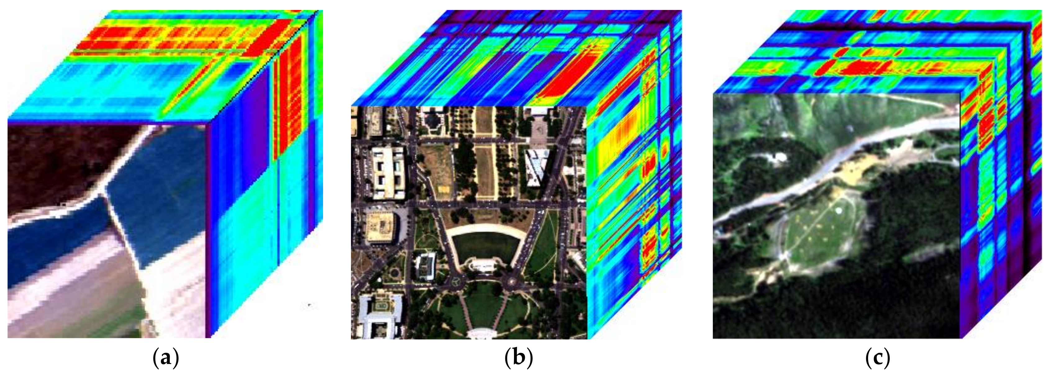
In this section, we first introduce the experimental datasets, and then we elaborate on the proposed resolution enhancement algorithm.

2.1. Datasets

Three synthetic groups of hyperspectral and multispectral datasets generated from real airborne HS images have been used to test the proposed technique. To evaluate the effectiveness of the proposed method, various scenes taken from different types of sensors are selected. The first HS data are taken over Salinas Valley, California, USA by the Airborne Visible Infrared Imaging Spectrometer (AVIRIS). The scene contains 512 × 217 pixels with 224 spectral bands in the wavelength range from 400 nm to 2500 nm. The second HS data are taken over Washington D.C., USA by the Hyperspectral Digital Imagery Collection Experiment (HYDICE) sensor. These data are characterized by 210 bands in the spectral range from 400 nm to 2400 nm and the scene contains 1208 × 307 pixels. The last scene is collected in the area around Montana, USA by a HyMap instrument provided by Rochester Institute of Technology (RIT), Henrietta, NY, USA [39]. The 126 spectral channels range from 453.8 nm to 2496.3 nm with a scene of 240 × 240 pixels selected. We select 120 × 120 pixels size of image of the first data with 204 spectral bands by removing water absorption region: 108–112, 154–167, 224. For the second dataset, a spatial size of 240 × 240 with 191 spectral channels by omitting atmosphere opaque region 103–106, 138–148, 207–210 remain. Figure 1 shows the experimental datasets.

The MS data are generated by spectrally downsampling of the HSS data corresponding to Landsat TM data, and the six bands cover a spectral range of 450–520, 520–600, 630–690, 760–900, 1550–1750 and 2080–2350 nm, respectively. The HS image is a spatially Gaussian downsampling of the HSS data with full-width at half maximum to a lower scale by a factor of 6. The downsampling factor is set as 6, which results in a sixfold difference in spatial resolution between two sensors, adopted and discussed in [15]. Considering that the spectral characters of synthetic images should be as identical as possible to the sensor with the highest spectral resolution [38], MS images are radiometrically calibrated to HS data according to the spectral degradation model and the parameters of the sensors.

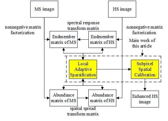
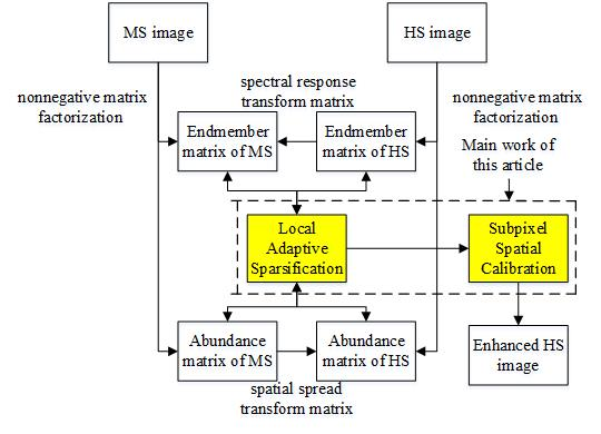
2.2. Local Adaptive Sparse Unmixing Based Fusion Approach

To obtain the HSS image $X_{HSS}\in {ℝ}^{b_h\times (r_m\times c_m)}$, a spectral signature of HS image $Y_{HS}\in {ℝ}^{b_h\times (r_h\times c_h)}$ and spatial features of the MS image $Y_{MS}\in {ℝ}^{b_m\times (r_m\times c_m)}$ are required. The 3D data cube are rearranged to a 2D matrix with each row representing all the pixels from a specific band, and each column representing the spectral signature at each pixel. $b_h$ and $b_m$ denote the numbers of spectral bands of HS and MS data, respectively. $c_h$ and $r_h$ denote the numbers of column and row pixels in HS data, respectively. $c_m$ and $r_m$ denote the numbers of column and row pixels in MS data, respectively.

Since the HS and MS images can be respectively considered as spatially and spectrally degraded versions of the HSS image, the sensor observation models that have been widely cited in [40,41,42] are given as:

$$Y_{HS}=X_{HSS}G+n_s,$$

(1)

$$Y_{MS}=L{X}_{HSS}+n_r,$$

(2)

where $G\in {ℝ}^{(r_m\times c_m)\times (r_h\times c_h)}$ denotes the spatial spread transform matrix, contains elements representing point spread function from MS to HS images, $L\in {ℝ}^{b_m\times b_h}$ is the spectral response transform matrix that represents the spectral response function from HS to MS images. $G$ and $L$ can be a priori known according to the sensors parameters, when applying to real data, $G$ is estimated by Gaussian point spread function, $L$ can be derived by cross calibration [27], and $n_s$ and $n_r$ are residuals.

A spectral unmixing technique is the decomposition of an image into a collection of constituent spectra called endmembers $E$, and a set of corresponding fractions called abundances $A$, and abundance maps indicate the proportion of individual endmember present in one pixel. With the advantages in physical effectiveness and mathematical simplicity, the linear spectral mixture model (LMM) [43] is the most commonly used model in solving the unmixing problems. It assumes that the spectrum of each pixel is a linear combination of spectral of several endmembers. Therefore, $X_{HSS}$ can be defined as:

$$X_{HSS}=E_{HS}{A}_{MS}+n,$$

(3)

where $E_{HS}=[e_{HS1},e_{HS2},\dots ,e_{HSd}]\in {ℝ}^{b_h\times d}$ is the endmember matrix of HS image, ${\left\{e_{HSi}\right\}}_{i=1}^d$ is the endmember spectrum and $d$ is the total number of endmembers. The multispectral image abundance map is $A_{MS}=[f_{MS1},f_{MS2},\dots ,f_{MS(r_m\times c_m)}]\in {ℝ}^{d\times (r_m\times c_m)}$, ${\left\{f_{MSi}\right\}}_{i=1}^{(r_m\times c_m)}$ is the endmember abundance fractions at each pixel and $(r_m\times c_m)$ is the total number of pixels. n represents the noise. By substituting LMM of $X_{HSS}$ defined by Equation (3) into the sensor observation models defined by Equations (1) and (2), $A_{HS}$ is the spatially degraded abundance matrix and can be derived as $A_{HS}=A_{MS}G$, and $E_{MS}$ is the spectrally degraded endmember matrix and can be derived as $E_{MS}=L{E}_{HS}$.

Unmixing based fusion techniques extract the endmembers from both data pairs and optimally calculate the high spatial resolution abundances accordingly. In previous works, such as CNMF and its derived methods, each pixel was regarded as the combination of all the endmembers according to LMM. To minimize the squared Frobenius norm of estimation residual matrices: ${\Vert Y_{HS}-E_{HS}{A}_{HS}\Vert }_F^2$ and ${\Vert Y_{MS}-E_{MS}{A}_{MS}\Vert }_F^2$, endmembers and abundances were alternately calculated by the multiplicative update rules. However, the endmember matrix is over completed for most local areas, so the update procedure may also force the noise $n_s$ and $n_r$ approximately represented by the linear mixture of the endmembers to reduce the residual and generate local full rank abundance matrices. Meanwhile, the endmembers of ground objects with small areas are gradually neglected for global optimization. The regions may also be fitted by the collinear endmembers as an ill-posed problem [44]. These will all impair the representation space of the endmembers, the spectral-spatial feature of the reconstructed HSS image and the convergence efficiency.

To deal with the problems above, a local adaptive sparse unmixing fusion (LASUF) method is proposed. The proposed algorithm attempts to further preserve the spectral composition characteristics of HS image and the spatial feature of MS image, by introducing priori geological constraints to the iterative solution of the coupled unmixing. At first, each pixel in the remote sensing images has finite cover scope, and thus contains a few categories of ground features. This means that the desired spectrum of each pixel is supposed to be mixed by a small number of endmembers. Consequently, the corresponding abundance matrix should be sparse. Secondly, the local correlation of the ground surface is respected in our procedure. That is, the distribution of ground objects has continuity to some extent and some category of object is more likely to appear around its congeneric areas. We suppose the abundance of one pixel indicates the existence probability of the endmembers, but not their exact composing proportion considering the noise. Thereupon, the abundance matrix can be regarded as a Markov Random Field, where the probability of the pixel x containing the n th endmember completely depends on abundance distribution of neighborhood $N_x$ centered on x:

$$P(A_x(n)>0|A_r,r\ne x)=P(A_x(n)>0|A_r,r\in N_x),$$

(4)

where $P(E_1|E_2)$ represents the conditional probability of one event $E_1$ occurring given that $E_2$ is already known, and $A_x(n)$ is the abundance of $n\mathrm{th}$ endmember at the position of x.

The distribution probability of the endmembers can be calculated as $P=A\otimes W$, $\otimes$ represents convolution operation, and $P\in {ℝ}^{d\times (r\times c)}$ and $W\in {ℝ}^{w\times w}$ are a Gaussian window with width of $w$. $P_x$ is a vector in dimension of $d\times 1$ with $P_x(i)$ representing the existence probability of the $i\mathrm{th}$ endmember at position x, and its sum is normalized to 1. Then, we construct a binary sparsification matrix $S\in {ℝ}^{d\times (r\times c)}$ utilizing P to make $A$ sparse. Considering that limited kinds of ground objects exist in one pixel, we suppose x is actually mixed by $q_x\ll d$ endmembers with greater existence probability, and other components are the approximate expression of noise n in Equations (1) and (2). The sparsification matrix $S$ is initialized as zero matrix and calculated as:

$$S_x(i)=\{\begin{array}{cc}1\hfill & P_x(i)\in {\max }_{q_x}(P_x)\mathrm{and}sum({\max }_{q_x}(P_x))\ge 1-\epsilon \\ 0\hfill & otherwise\end{array},$$

(5)

where $\epsilon$ is the permissible error of unmixing reconstruction. When the sum of largest $q_x$ probabilities is higher than $1-\epsilon$, the corresponding elements in $S_x$ are set to “1” and others remain as “0”. The objective function of the optimization problem can be formulated as minimization of the global estimation residual constrained by the priori sparsity:

$$\begin{array}{c}\min \frac{1}{2}{\Vert Y_{HS}-E_{HS}{A}_{HS}\Vert }_F^2+\frac{1}{2}{\Vert Y_{MS}-E_{MS}{A}_{MS}\Vert }_F^2\\ s.t.q_{HS}\ll d\mathrm{and}{q}_{MS}\ll d\mathrm{and}{E}_{HS},A_{HS},E_{MS},A_{MS}\ge 0\end{array}.$$

(6)

The proposed LASUF algorithm is summarized in Algorithm 1. The endmembers and abundance matrix are initialized using the input HS and MS data by endmember extraction and fully constrained least squares (FCLS) method [45]. Considering the good robustness of unmixing iteration procedures to the initial endmember extraction result, which has been discussed in the previous work [32], various kinds of endmember extraction methods can be used including vertex component analysis (VCA), N-finder algorithm (N-FINDR), pure pixel index (PPI), etc. In addition, VCA [46] is adopted for all of the fusion methods for a fair comparison in our experiments, since it is a state-of-the-art endmember extraction method that does not require the presence of pure pixels in the image. Then, through introducing the sparse and local correlation constraint to each inter-optimization iteration of the unmixing procedure, the sparsification matrix of the MS image and HS image are calculated as:

$$P_{HS}\leftarrow A_{HS}\otimes W,$$

(7)

$$S_{H{S}_x}(i)=\{\begin{array}{cc}1\hfill & P_{H{S}_x}(i)\in {\max }_{q_x}(P_{H{S}_x})\mathrm{and}sum({\max }_{q_x}(P_{H{S}_x}))\ge 1-\epsilon \\ 0\hfill & otherwise\end{array},$$

(8)

and

$$P_{MS}\leftarrow A_{MS}\otimes W,$$

(9)

$$S_{M{S}_x}(i)=\{\begin{array}{cc}1\hfill & P_{M{S}_x}(i)\in {\max }_{q_x}(P_{M{S}_x})\mathrm{and}sum({\max }_{q_x}(P_{M{S}_x}))\ge 1-\epsilon \\ 0\hfill & otherwise\end{array}.$$

(10)

Then, the local adaptive sparse abundance matrix is calculated as:

$$A_{HS}^S\leftarrow A_{HS}.\ast S_{HS},$$

(11)

$$A_{MS}^S\leftarrow A_{MS}.\ast S_{MS}.$$

(12)

Unlike the sparse method in [33,34,35], endmembers are updated in the iterative optimization utilizing local sparsity of ground objects distribution along with the spatial correlation between MS and HS images via Lee and Seung’s multiplicative update rules [47], which are given as:

$$E_{HS}\leftarrow E_{HS}.\ast (Y_{HS}{(A_{HS}^S)}^T)./(E_{HS}{A}_{HS}^S{(A_{HS}^S)}^T),$$

(13)

$$A_{HS}\leftarrow A_{HS}^S.\ast (E_{HS}^T{Y}_{HS})./(E_{HS}^T{E}_{HS}{A}_{HS}^S),$$

(14)

$$E_{MS}\leftarrow E_{MS}.\ast (Y_{MS}{(A_{MS}^S)}^T)./(E_{MS}{A}_{MS}^S{(A_{MS}^S)}^T),$$

(15)

$$A_{MS}\leftarrow A_{MS}^S.\ast (E_{MS}^T{Y}_{MS})./(E_{MS}^T{E}_{MS}{A}_{MS}^S),$$

(16)

where ${(\cdot )}^T$ denotes the transposition of the matrix and ∗ and ./ denote elementwise multiplication and division, respectively.

In LASUF, we can gradually acquire the local adaptive optimal solution instead of global optimization. Therefore, the endmembers of small ground objects are harder to ignore, for their abundances in other areas are set to zero and barely contribute to the overall estimation residual. The endmembers matrix $E_{HS}$ and $E_{MS}$ become more expressive than the previous unmixing procedure consequently.

Algorithm 1 Local Adaptive Sparse Unmixing Based Fusion

1: Input: Hyperspectral data $Y_{HS}$ and multispectral data $Y_{MS}$, degradation matrix L and G, permissible error $\epsilon$ 2: initialization stage 3: Endmember extraction from $Y_{HS}$ to initialize $E_{HS}$ by VCA. 4: Initialize $A_{HS}$ from $Y_{HS}$ and initial $E_{HS}$ by using the FCLS method. 5: Initialize $E_{MS}$ from $E_{HS}$ by $E_{MS}=L{E}_{HS}$. 6: Initialize $A_{MS}$ from $Y_{MS}$ and initial $E_{MS}$ by using the FCLS method. 7: Optimization stage 8: Outer loop for 9: Inter loop1 Sparse optimize LHS (Iteration until convergence) 10: generate the sparsification matrix $S_{HS}$ from $A_{HS}$ by (7) and (8) 11: generate the local adaptive sparse abundance matrix $A_{HS}^S$ for $Y_{HS}$ by (11) 12: Optimize $E_{HS}$ using the sparse abundance matrix $A_{HS}^S$ by (13). 13: Optimize $A_{HS}$ by using (14) 14: end 15: Update $E_{MS}$ from $E_{HS}$ by $E_{MS}=L{E}_{HS}$. 16: Inter loop2 Sparse optimize HMS (Iteration until convergence) 17: generate the sparsification matrix $S_{MS}$ from $A_{MS}$ by (9) and (10) 18: generate the local adaptive sparse abundance matrix $A_{MS}^S$ for $Y_{MS}$ by (12) 19: Optimize $E_{MS}$ using the sparse abundance matrix $A_{MS}^S$ by (15). 20: Optimize $A_{MS}$ by using (16) 21: end 22: Update $A_{HS}$ from $A_{MS}$ by $A_{HS}=A_{MS}G$ 23: end for 24: fusion stage 25: Fuse $E_{HS}$ and $A_{MS}$ by using $X_{HSS}=E_{HS}{A}_{MS}$ to get HSS. 26: Output: fused high spatial-spectral resolution hyperspectral image $X_{HSS}$.

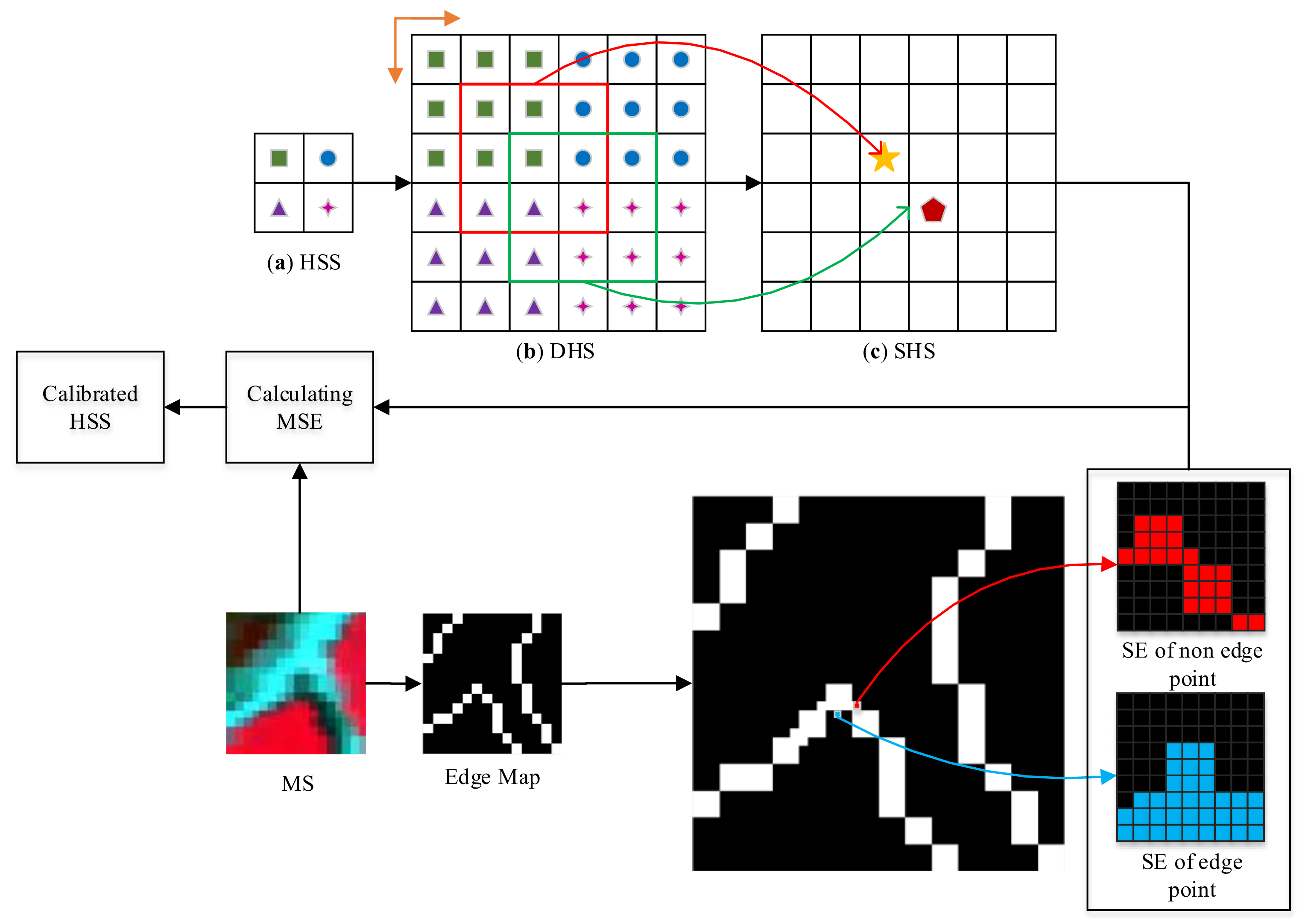
2.3. Subpixel Spatial Calibration Phase

The existing fusion approaches, including unmixing based methods, generally expect that the observed high spatial resolution MS and low spatial resolution HS images are geometrically coregistered with radiometric correction. That is, each pixel in HS spatially corresponds to $(r_m/r_h)\times (c_m/c_h)$ entire pixels in MS exactly, as shown in Figure 2a. Unfortunately, in practical application, the integer-pixel matching is difficult to achieve due to different sensors, platform, and atmospheric refraction conditions [48]. On one side, with the development of an unmanaged autonomous vehicle (UAV) technique, airborne sensors provide a major source of high-resolution remote sensing images. However, due to airstream and flight control, the airborne platform route cannot maintain adequate precision like a satellite. Consequently, subpixel misalignment may appear in some local areas as shown in Figure 2b. On the other side, except for the same multi-sensor platform, HS and MS images are generally captured in different time phases. Ground objects and atmospheric condition probably change as time goes by, such as movements of man-made cars or boats, evolution of vegetation, waves or coastlines. This may lead to the accidental subpixel shift as shown in Figure 2c and the anamorphic misregistration in Figure 2d. Even HS and MS images can be absolutely precisely calibrated, the fusion processes are likely to introduce some random subpixel shift between HSS and MS images. The existing fusion procedure attempts to minimize the squared norm of estimation residual matrices and obtain the global optimization, but ignores the local accuracy at the pixel level. In addition, fusion methods usually assume that the underlying surface is a plane and a diffuse reflect incident electromagnetic wave; therefore, it conforms to the Gaussian mixture model. While the hypothesis may not be entirely accurate, for instance, when there exists slope, specular reflection or ground features that have obvious absorption of some certain bands, mixed pixels in an HS image are not simply a Gaussian mixture of pure pixels. The unmixed result also has spatial bias. If these factors are considered in the unmixing model, the fusion algorithm complexity will be greatly increased. Considering that the MS image has more accurate and reliable spatial information, we expect to correct the HSS image on the subpixel level to make it have spatial features in accordance with the MS image and preserve its spectrum composition characteristics simultaneously. Hence, we design a subpixel calibration postprocessing to solve the above problem and further improve the fusion accuracy.

In this section, an optimal matching based adaptive morphology filtering (OM-AMF) using MS data as the reference is proposed for subpixel spatial calibration of the HSS image. Traditional mathematical morphology can explore and calibrate specific morphological structure in a gray scale image utilizing a structuring element (SE) and sorting operator [49]. The erosion result of an image $f(x)$ with an SE is the minimum value of the pixels in the scope of SE when its origin is at x:

$${\epsilon }_{SE}[f(x)]=\underset{b\in SE}{\min } f(x+b),$$

(17)

where ${\epsilon }_{SE}(\cdot )$ denotes the erosion operator, and $b$ indicates the vectors from x to the pixels in SE.

Equation (17) can be rewritten as an optimization form:

$$\{\begin{array}{l}{\epsilon }_{SE}[f(x)]=f(x+\widehat{b})\\ \widehat{b}=\underset{b\in SE}{\arg \min } f(x+b)\end{array},$$

(18)

where $\widehat{b}$ represents the position vector from $x$ that minimizes the object function $f(\cdot )$.

Then, we extend the optimization form of morphology to the condition with reference data to match. The filtering result of optimal matching (OM) morphology can be defined as the pixel in the SE with the minimum mean square error (MSE) of the corresponding pixel in the reference image:

$$\{\begin{array}{l}{\psi }_{SE}[C(x_c),R(x_r)]=C(x_c+\widehat{b})\\ \widehat{b}=\underset{b\in SE}{\arg \min } MSE(C(x_c+b),R(x_r))\end{array},$$

(19)

where ${\psi }_{SE}[C,R]$ denotes the OM morphology operator of the input data $C$ and the reference data $R$, and $x_c$ and $x_r$ are the corresponding positions in $C$ and $R$; when $C$ and $R$ are cube data, $MSE(C(x_c+b),R(x_r))$ represents the mean square error of the vectors at $x_c+b$ and $x_r$. $\widehat{b}$ represents the position vector from $x_c$ that minimizes the MSE of $C(x_c+b)$ and $R(x_r)$ in the scope of SE.

We take advantage of the OM morphology and adaptive structuring element (ASE) to adjust the spatial structure of HSS data in accordance with the MS image. The flowchart is shown in Figure 3. At first, the subpixels of the HSS image, with the identical spectrum components, are constructed. We divide each pixel into $k\times k$ subpixels in space to get a dense hyperspectral image (DHS, $X_{DHS}\in {ℝ}^{k^2{b}_h\times (r_m\times c_m)}$) as shown in Figure 3b. Then, each pixel in DHS is replaced by the average linear mixture of its $k\times k$ neighborhood to obtain a spatial overcomplete hyperspectral image (SHS, $X_{SHS}\in {ℝ}^{k^2{b}_h\times (r_m\times c_m)}$), as shown in Figure 3c. One pixel in the SHS map contains the same spatial scope as the pixel in the MS image and is centered at the corresponding position of the subpixel in the DHS image. Meanwhile, the SHS map can also be linear represented by $E_{HS}$.

To preserve the spatial character of MS image, the edge constrained 4-neighbour growth is used to generate the ASE for an SHS image constraint by the edge of the MS image [50,51]. PCA transformation is executed on the MS image, and the edge map is detected by implementing a Sobel operator on the $k\times k$ super-resolution of the largest PCA component. Then, ASE is constructed for each pixel of the SHS image to reveal its homogenous region. Finally, the OM-AMF is executed to update the HSS image with the pixel in the ASE scope of SHS data, whose spectrum degeneration has the minimum MSE with the corresponding pixel in MS image:

$$\{\begin{array}{l}{X}_{HSS}^{\prime }(z_h)={\psi }_{ASE}[X_{SHS}(z_s),Y_{MS}(z_h)]=X_{SHS}(z_s+\widehat{b})\\ \widehat{b}=\underset{b\in ASE}{\arg \min }\mathrm{MSE}(L{X}_{SHS}(z_s+b),Y_{MS}(z_h))\end{array},$$

(20)

where $z_h$ is the position of the pixel to be operated in the HSS image and $z_s$ is the corresponding position in the SHS image; ASE is the adaptive structuring element generated via the edge of the MS image. For the spectral response transform matrix, $L$ is the same as the fusion procedure and has been cross calibrated, and the overall radiation consistency of $L{X}_{SHS}$ and $Y_{MS}$ is receivable. Denoising process should be executed on the MS data firstly to reduce the risk of radiation deviation for the proposed subpixel calibration.

Most fusion methods, including the proposed LASUF, provide overall or local optimal estimation from MS and HS images. Due to the low spatial resolution of HS data, they can hardly achieve the best spatial resolution on the level of high spatial resolution pixels. The better matched results may be found in the neighbor subpixels. Consequently, the proposed OM-AMF can improve the results of most fusion procedures even though the MS and HS images are completely matched in spatial dimension.

3. Experimental Results

3.1. Experimental Setup

The proposed LASUF-OM method is applied to the above datasets. To demonstrate the effectiveness of the proposed method, four representative methods are compared as competitors, including MAP [19], CNMF [26], Bayesian [22], and NSSR [35]. The parameters of these methods were manually adjusted to the optimal. In CNMF and LASUF-OM, the maximum number of iterations for inner and outer loops are set to 200 and 3. The thresholds for the convergence condition are set at ${10}^{-6}$ and their endmembers are initialized via VCA with the same number at 30 empirically referring to [15]. This number and the final performance depend on the scene complexity of the images in practical application. Particularly, for the proposed method, the permissible error of the local adaptive sparse process is set as $\epsilon =0.1$; the maximum radius ASE is 5, while, in MAP, six PCs, four endmembers, and 20 mixture classes are adopted. The regularization parameter of Bayesian is fixed as 0.0001. The number of atoms in the dictionary in NSSR is set as 80, and iteration numbers and convergence thresholds are set as in the reference. The processor Intel (R) Core (TM) i7 CPU 2.40 GHz RAM 12 GB is selected for all experiments.

In addition, the ideal estimated HSS image should preserve the spectral information of the HS image and the spatial information of the MS image, and both qualitative and quantitative assessments are adopted to overall evaluate the performance from those two aspects. Some typical bands and spectral profiles are presented as visual indices, and the quantitative measurements are evaluated between the generated HSS data and the original reference image, including the spatial measure of the peak signal-to-noise ratio (PSNR) index and cross correlation (CC) index, a spectral measure of the spectral angle mapper (SAM) index and a global measure of the erreur relative globale adimensionnelle de synthése (ERGAS) index [52]. The definition of PSNR is as follows:

$$PSN{R}_k=10\ast {\log }_{10}\frac{Ma{x}_k^2{\mathrm{r}}_{\mathrm{m}}{\mathrm{c}}_{\mathrm{m}}}{{\displaystyle \sum _{i=1}^{{\mathrm{r}}_{\mathrm{m}}}{\displaystyle \sum _{j=1}^{{\mathrm{c}}_{\mathrm{m}}}{[{\widehat{X}}_{HSS}^k-X_{HSS}^k]}^2}}},$$

(21)

where ${\widehat{X}}_{HSS}^k$ denotes a single band of the estimated HSS image, and $X_{HSS}^k$ denotes a single band of the reference HSS image. $Ma{x}_k$ is the maximum pixel value in the kth band image. The CC index characterizes the geometric distortion between estimated and reference data, the optimal value of CC is 1, and it is defined as:

$$CC=\frac{1}{b_h}{\displaystyle \sum _{k=1}^{b_h}\frac{{\displaystyle \sum _{i=1}^{{\mathrm{r}}_m}{\displaystyle \sum _{j=1}^{{\mathrm{c}}_m}({\widehat{X}}_{HSS}^k-{\mu }_{\widehat{X}}^k)(X_{HSS}^k-{\mu }_X^k)}}}{\sqrt{{\displaystyle \sum _{i=1}^{{\mathrm{r}}_m}{\displaystyle \sum _{j=1}^{{\mathrm{c}}_m}{({\widehat{X}}_{HSS}^k-{\mu }_{\widehat{X}}^k)}^2{(X_{HSS}^k-{\mu }_X^k)}^2}}}}},$$

(22)

where ${\mu }_{(·)}$ denotes the sample mean. SAM measures the spectral shape preservation by calculating the distance between two spectral vectors of two pixels, and it is defined as:

$$SAM=\arccos \left(\frac{\langle x,\widehat{x}\rangle }{{\Vert x\Vert }_2{\Vert \widehat{x}\Vert }_2}\right),$$

(23)

where $x$ and $\widehat{x}$ denote the spectral vector of reference and estimated HSS images, respectively. $\langle x,\widehat{x}\rangle =x^T\widehat{x}$ is the inner product. The lower SAM means the lower spectral distortion and the optimal value is 0. ERGAS evaluates the global quality of the estimated HSS image and is defined as:

$$ERGAS=100d\sqrt{\frac{1}{b_h}{\displaystyle \sum _{k=1}^{b_h}{\left(\frac{RMS{E}^k}{{\mu }_X^k}\right)}^2}},$$

(24)

$$RMSE=\frac{{\Vert {\widehat{X}}_{HSS}-X_{HSS}\Vert }_F}{\sqrt{b_h\times r_m\times c_m}},$$

(25)

where $d$ is the spatial resolution ratio from HSS to HS images, and RMSE is the well-known root mean square error that computes spatial quality. By calculating each band, the spectral information quality is considered, and the optimal value is 0.

3.2. Integer Pixel Matched Fusion Experiment

At first, we assume that the MS and HS images are completely matched with no subpixel shift. The space enhancement ratio in OM-AMF postprocessing is set as $k=3$. In

Table 1. Comparison of average statistical indexes of different methods of data Salinas.

Dataset	Index	PSNR (dB)	SAM (rad)	CC	ERGAS	Time (s)
Salinas	MAP	32.9592	0.0187	0.9877	0.9536	6.68
	CNMF	35.2277	0.0128	0.9869	0.9197	70.79
	Bayesian	35.7891	0.0141	0.9896	0.8319	6.79
	NSSR	37.1807	0.0113	0.9871	0.7883	50.81
	LASUF	39.4132	0.0095	0.9899	0.7737	18.08
	LASUF-OM	40.0492	0.0091	0.9901	0.7639	39.72

PSNR: peak signal-to-noise ratio; SAM: spectral angle mapper; CC: cross correlation; ERGAS: erreur relative globale adimensionnelle de synthése; MAP: maximum a posteriori; CNMF: coupled nonnegative matrix factorization; NSSR: non-negative structured sparse representation; LASUF: local adaptive sparse unmixing fusion; LASUF-OM: local adaptive sparse unmixing fusion and optimal matching.

,

Table 2. Comparison of average statistical indexes of different methods of data Washington D.C.

Dataset	Index	PSNR (dB)	SAM (rad)	CC	ERGAS	Time (s)
Washington D.C.	MAP	38.7546	0.0354	0.9889	1.7922	6.85
	CNMF	37.1528	0.0268	0.9858	1.8408	78.38
	Bayesian	37.8320	0.0316	0.9875	1.414	7.73
	NSSR	38.7432	0.0274	0.9894	1.7245	61.77
	LASUF	38.3789	0.0249	0.9923	1.3383	16.77
	LASUF-OM	40.8441	0.0226	0.9924	1.3041	38.06

and

Table 3. Comparison of average statistical indexes of different methods of Montana data.

Dataset	Index	PSNR (dB)	SAM (rad)	CC	ERGAS	Time (s)
Montana	MAP	41.8429	0.0204	0.9935	1.577	14.73
	CNMF	43.6353	0.0196	0.9922	1.7007	230.39
	Bayesian	43.8688	0.0193	0.9934	1.5844	9.97
	NSSR	44.1863	0.0202	0.9917	1.7156	121.25
	LASUF	49.0741	0.0145	0.9939	1.4636	72.86
	LASUF-OM	49.5409	0.0136	0.9942	1.4323	109.27

, the average statistical indexes of the PSNR, SAM, CC, and ERGAS values and the running time of all the tested methods are given for the three pairs of datasets. Globally, these tables show that the proposed LASUF-OM algorithm has remarkable results in both spectral and spatial perspectives.

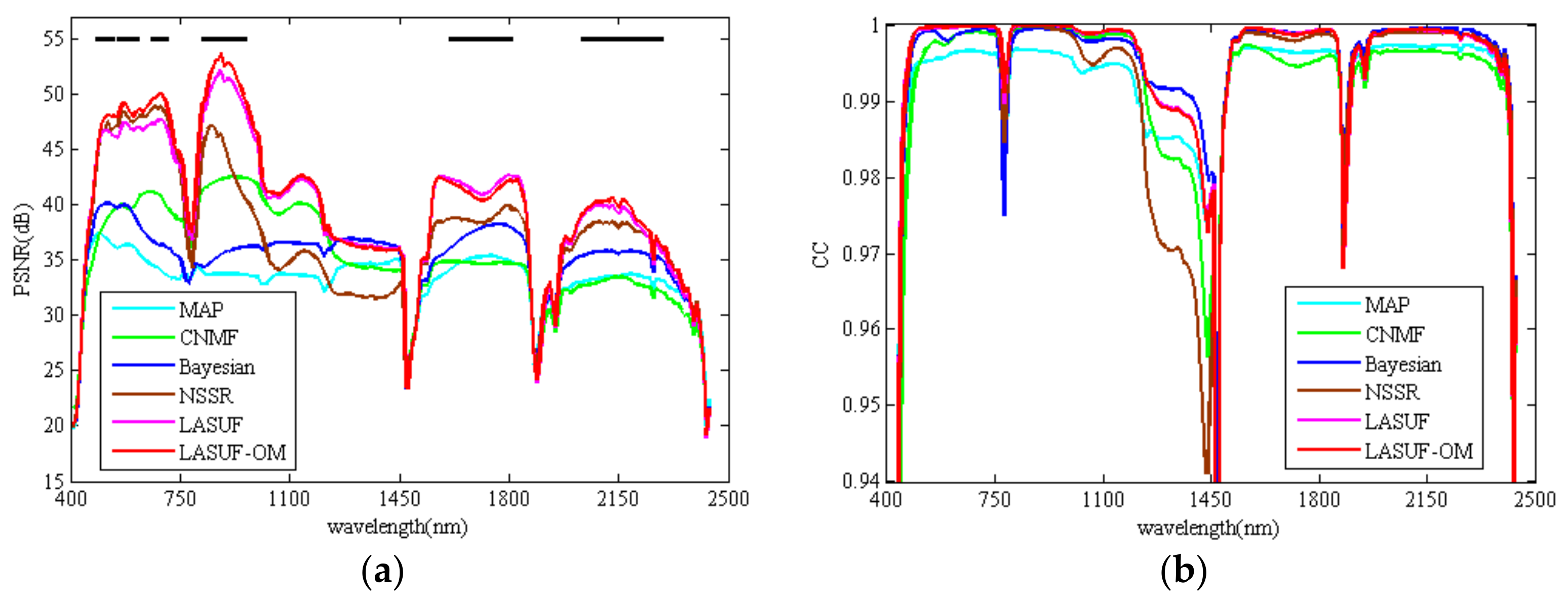
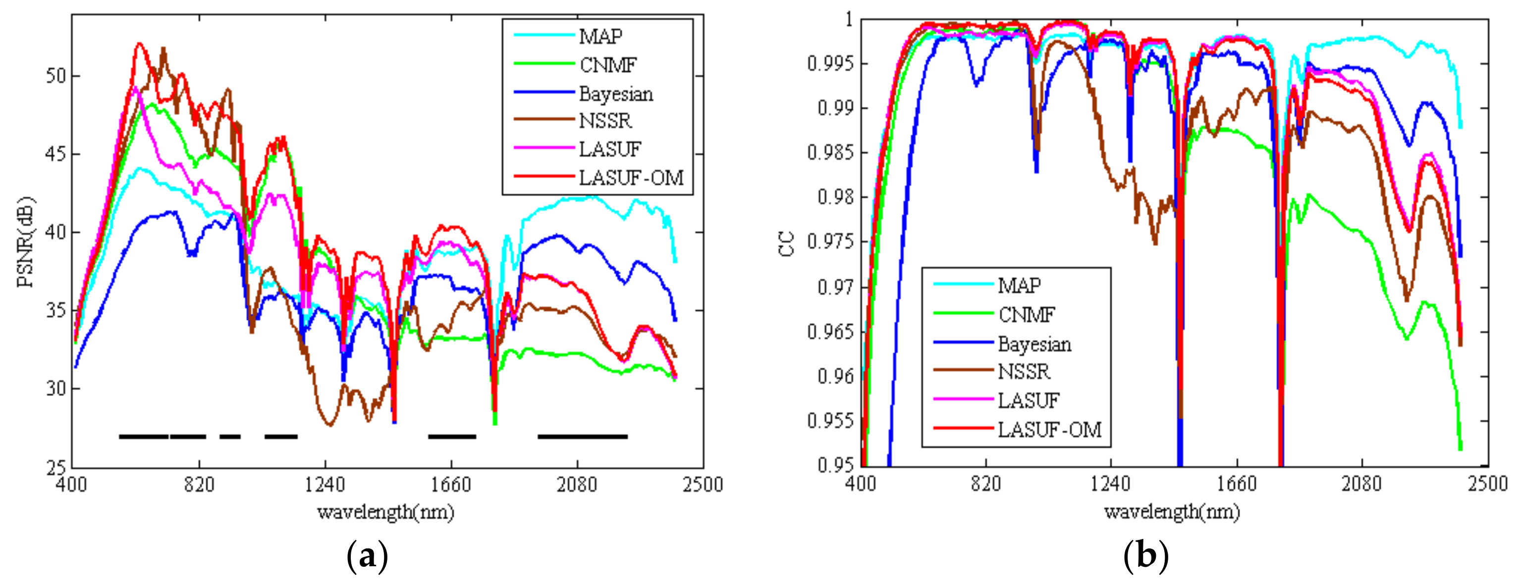
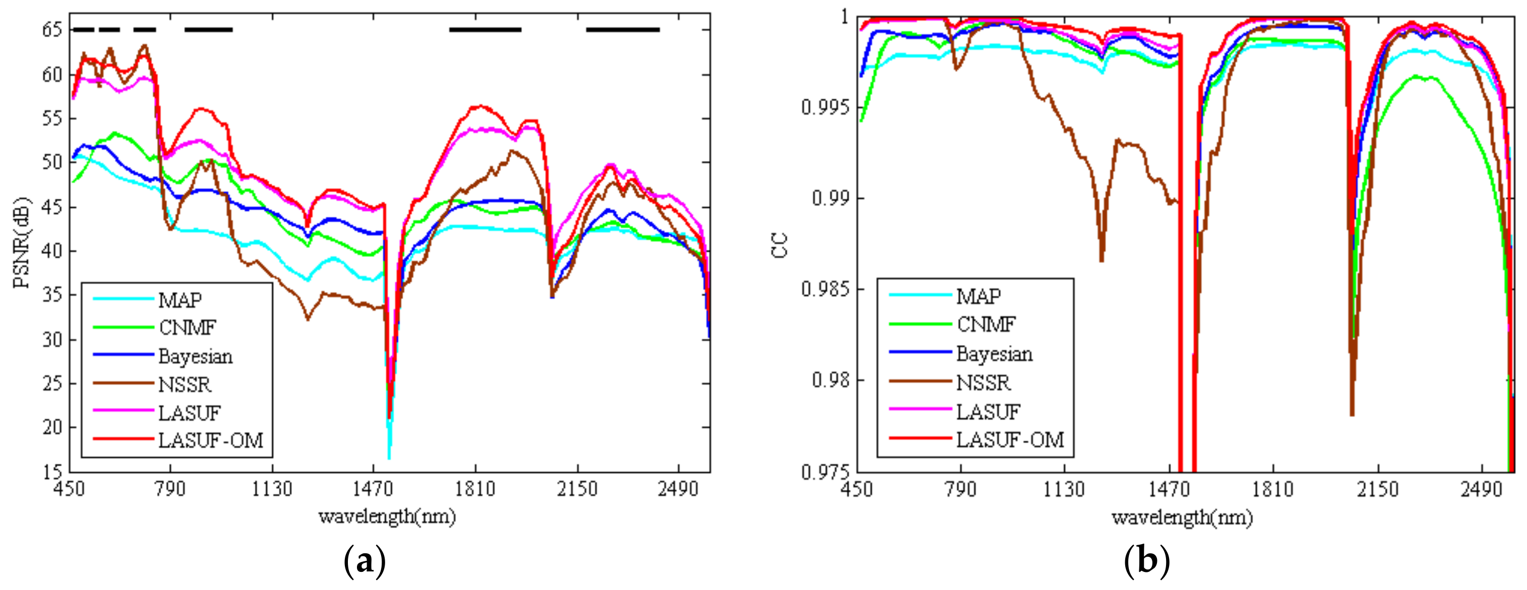
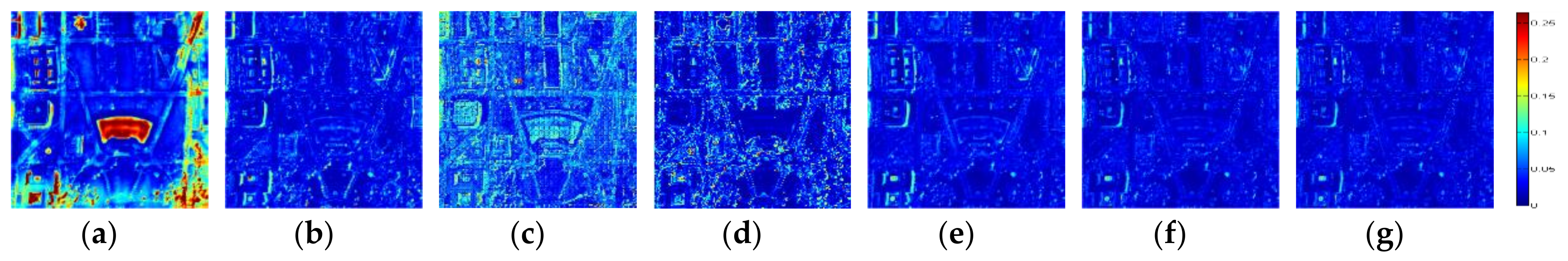
3.2.1. From the Spectral Viewpoint

As indicated in Table 1, Table 2 and Table 3, the proposed LASUF method presents lower overall SAM values. After the postprocessing of OM-AMF, the SAM values are further reduced. It means that the OM-AMF is valuable even though no subpixel shift exists, as the fusion methods provide overall or local optimum estimation and better results may be found in the neighbor subpixels. Figure 4, Figure 5 and Figure 6 show the corresponding SAM heat maps, which reveal spatial distribution of the spectral errors for each pixel. It can be observed that there are many small spots with warm color in the SAM maps of MAP, which indicate that greater spectral distortion exists in these reconstruction areas. For CNMF, these warm pixels mean that the spectrum of these small separate areas can hardly be perfectly expressed by the final endmembers of the iterative unmixing procedures. The average SAM value of Bayesian is high since the spectral physical property is not considered, and the warm color and block effect of the SAM map also prove that. Although NSSR has a relatively small average SAM value, the warmer areas of spatial structure details in the SAM map illustrate that the NSSR method is not suitable for regions with distinct spectral mixing. Nevertheless, the SAM maps of the LASUF and LASUF-OM are almost all blue and have barely warm areas. It demonstrates that the local adaptive sparsification can preserve the spectral composition of isolated ground objects, making use of the local correlation and sparsity of the ground features in limited areas. Our unmixing update procedure achieves local optimization adaptively and the impact from nonlocal or non-homogeneous regions for the global optimum are avoided by the sparse abundance matrix. In addition, in the OM-AMF calibration, the subpixels for selection are generated strictly according to the rule of LMM; hence, spectral signatures stay unchanged after subpixel calibration.

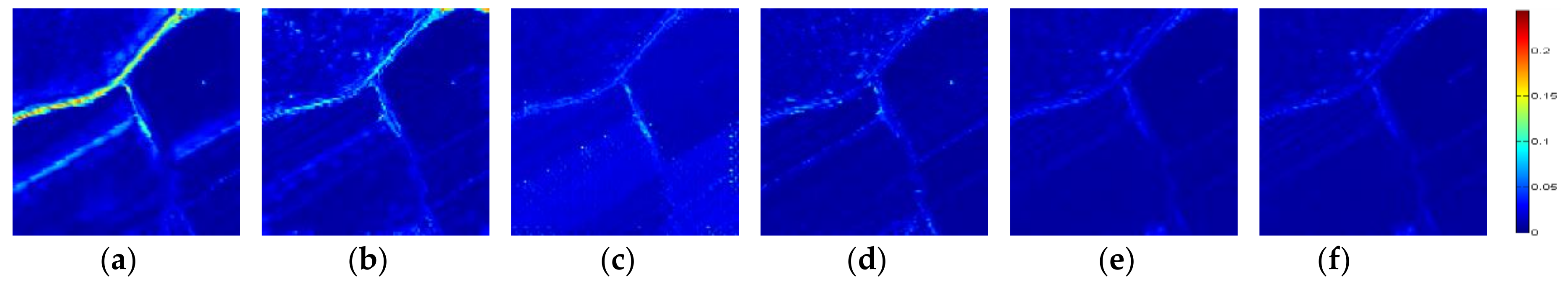
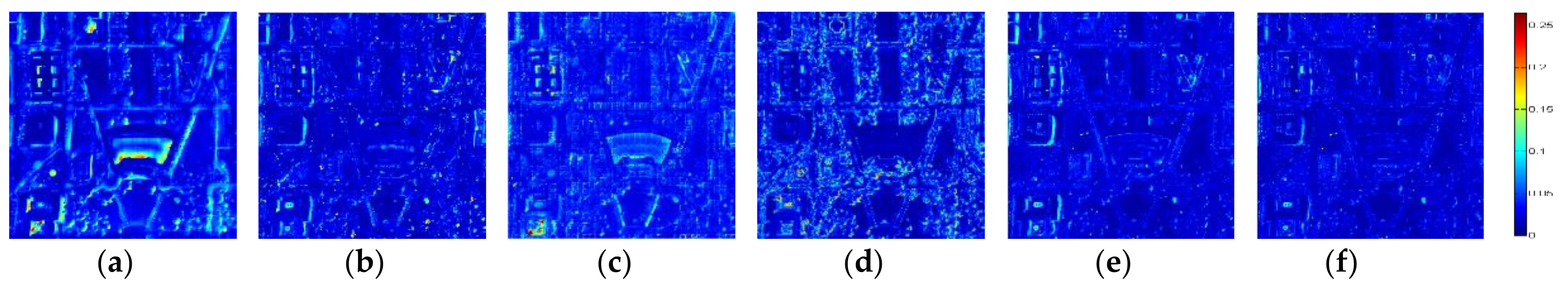
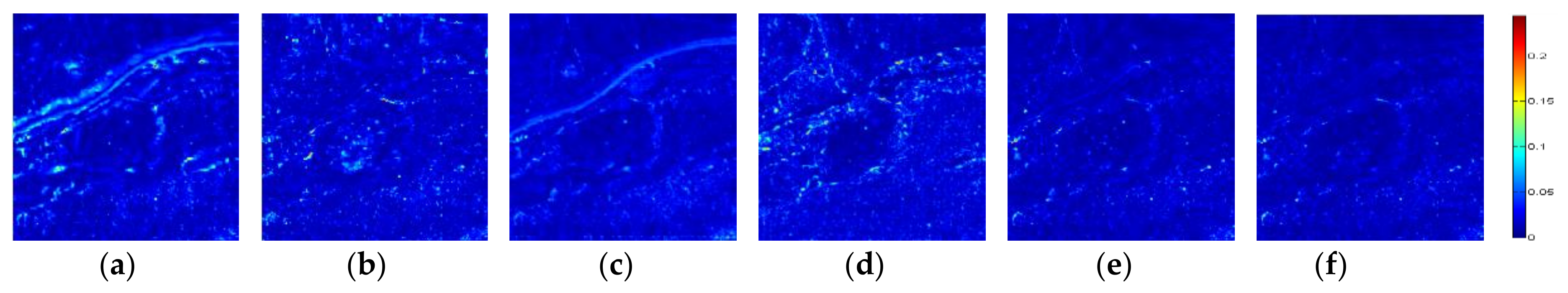
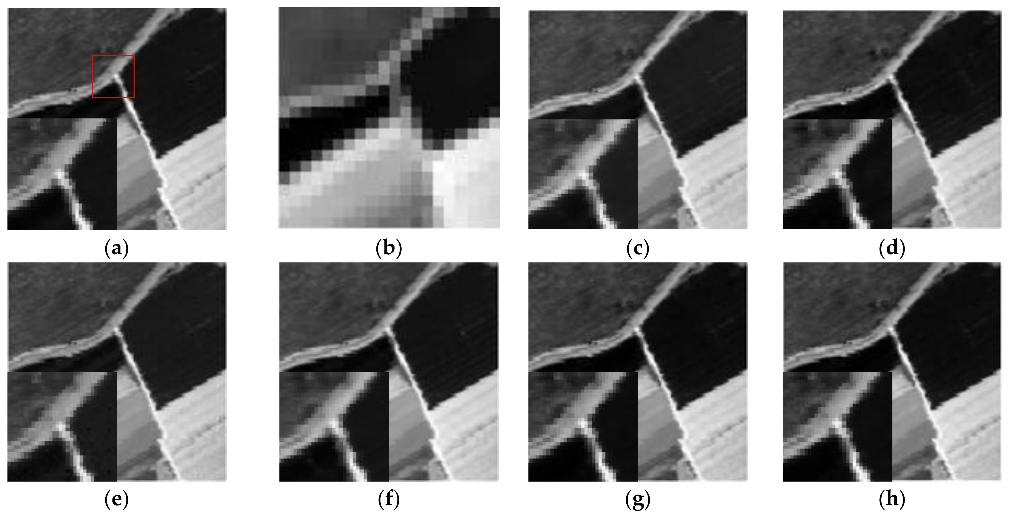
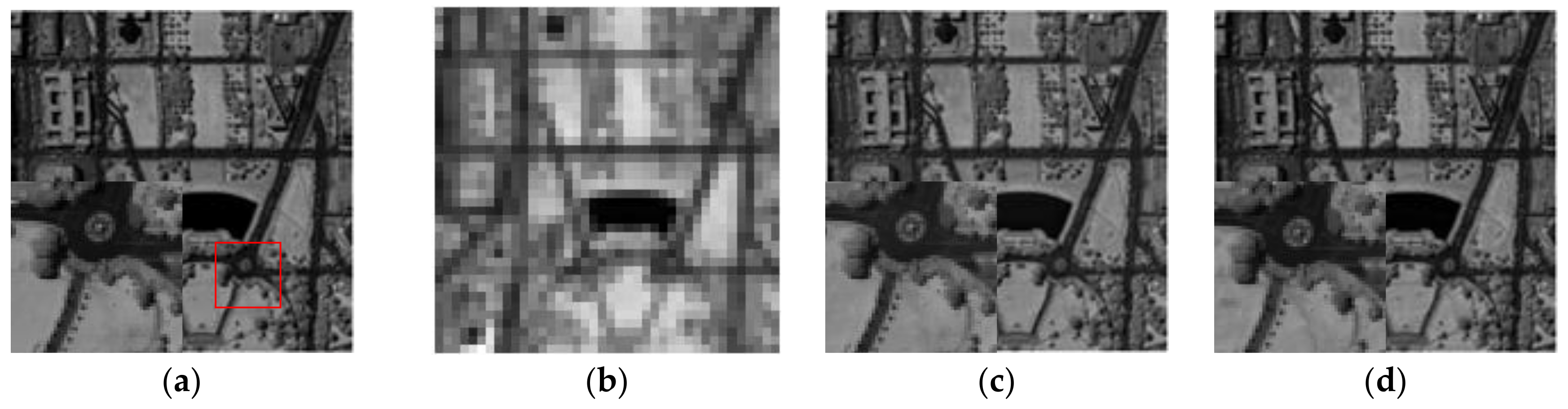
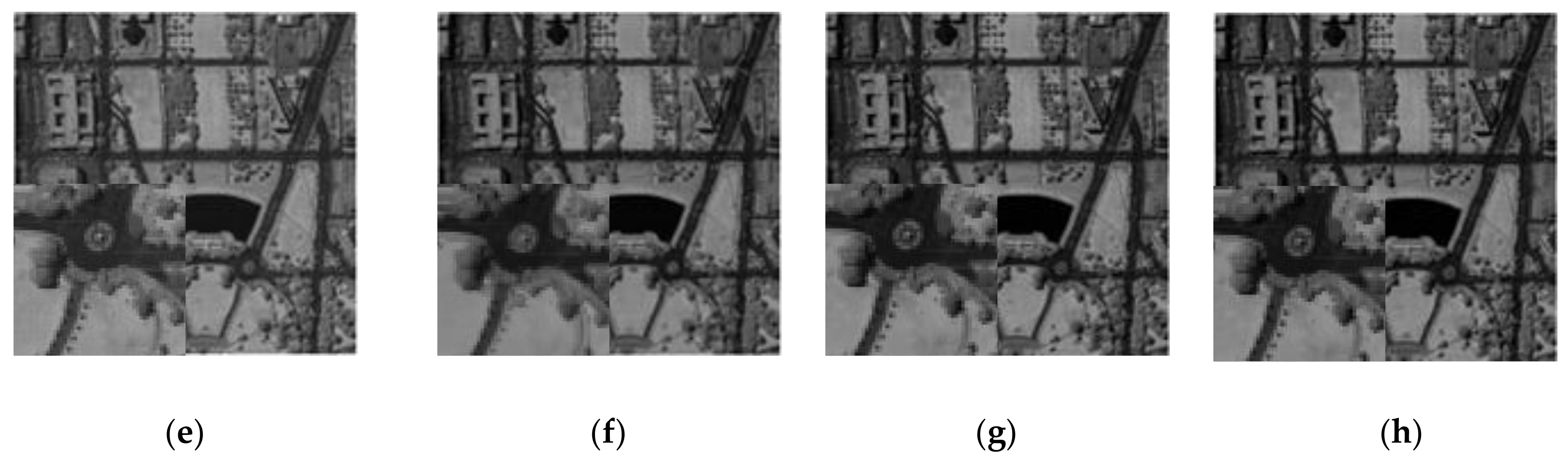
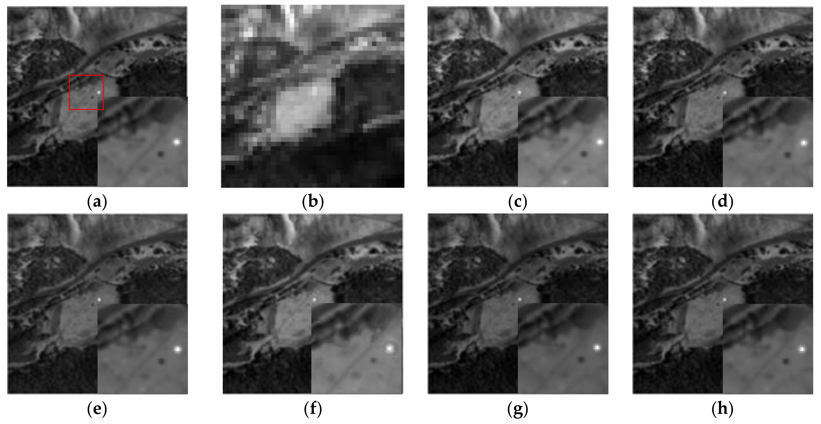
3.2.2. From the Spatial Viewpoint

To further analyze the relationship between the spatial fusion quality and the wavelength, the comparisons of PSNR and CC curves for each band of the HSS data are shown in Figure 7, Figure 8 and Figure 9, and the wavelength distributions of the MS data are also marked in the PSNR curves. It can be seen that fusion results of all the methods are more ideal in the spectrum wavelength range that have overlapping parts between MS and HS images. Results of the Bayesian estimator have relatively poor sensitivity compared to other methods, while NSSR has great fusion results. In bands with no corresponding MS wavelength, the fusion effect of the HSS image falls sharply, and NSSR results in 1100–1400 nm perform the worst. The proposed method shows better results in the different wavelength regions. It can also be observed that the CC of our method is closest to the ideal value 1, and the slightest geometric distortion is introduced by the proposed method. In addition, the superiorities in the non-repetitive bands are even more obvious, which demonstrates better spectral enhancement capability of the proposed method. For visual comparison, Figure 10, Figure 11 and Figure 12 show the grayscale images and their local details of the reference, low resolution HS images and the resolution enhanced results for MAP, CNMF, Bayesian, NSSR and the proposed algorithm, with the wavelength of 1541 nm, 1204 nm and 1190 nm, respectively, for Salinas, Washington D.C. and Montana data. It can be visibly perceived that, for the non-repetitive wavelength, the fusion results of the proposed LASUF-OM method are the closest to the reference data by visual inspection. The local details include that the grayscale and shape features are maintained well in our results.

In general, high spectral spatial resolution hyperspectral data obtained by the proposed LASUF-OM strategy maintains the spectral signature of hyperspectral image and embodies the spatial features of multispectral images. The global measure ERGAS index also emphasizes this fact.

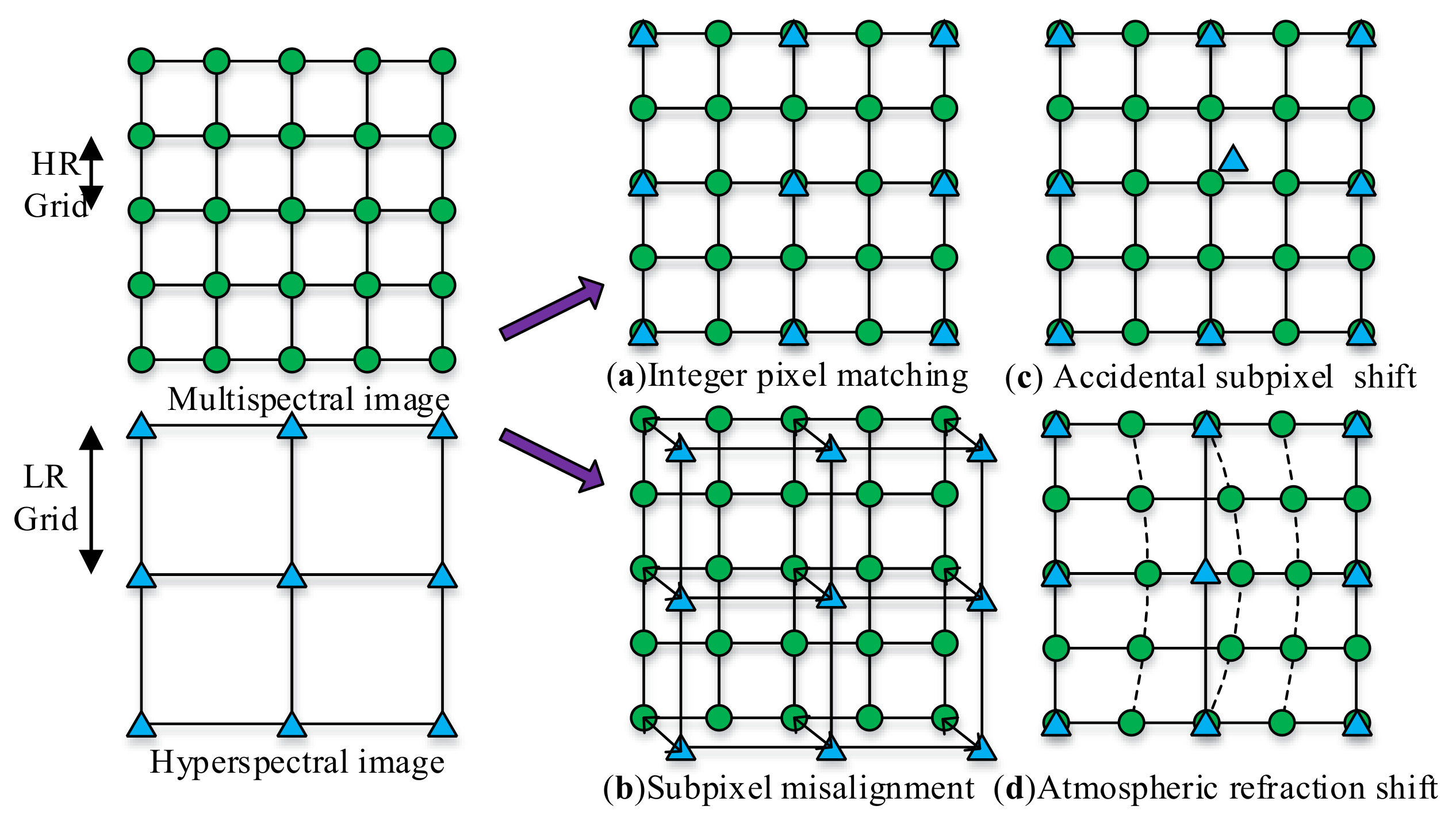
3.3. Subpixel Shift Experiment

A subpixel shift experiment is designed to further verify the performance of the proposed OM-AMF based subpixel calibration algorithm. In addition, $1/3\times 1/3$ and $1/2\times 1/2$ of the high spatial resolution pixel shift are manually added into HS Washington D.C. data along the low right side to discuss the influence of subpixel shift to various fusion methods.

Statistical indexes of the fusion results on the two shift datasets obtained by MAP, CNMF, Bayesian, NSSR, LASUF and LASUF-OM with k = 3, k = 6 are given respectively in

Table 4. Comparison of average statistical indexes of different methods of Washington D.C. (1/3 Subpixel Shift).

Dataset	Index	PSNR (dB)	SAM (rad)	CC	ERGAS
Washington D.C.	MAP	35.4668	0.0664	0.9887	1.9176
	CNMF	35.8417	0.0321	0.9838	1.8451
	Bayesian	34.8561	0.0598	0.9780	1.7198
	NSSR	35.7487	0.0356	0.9865	1.7901
	LASUF	37.2507	0.0284	0.9911	1.4886
	LASUF-OM, k = 3	38.7873	0.0251	0.9913	1.4139
	LASUF-OM, k = 6	39.1114	0.0244	0.9916	1.3879

and

Table 5. Comparison of average statistical indexes of different methods of Washington D.C. (1/2 Subpixel Shift).

Dataset	Index	PSNR (dB)	SAM (rad)	CC	ERGAS
Washington D.C.	MAP	35.1011	0.0694	0.9880	2.0194
	CNMF	35.3238	0.0371	0.9737	1.9078
	Bayesian	34.7970	0.0607	0.9775	1.7349
	NSSR	35.3824	0.0396	0.9845	1.9528
	LASUF	36.4405	0.0303	0.9904	1.5454
	LASUF-OM, k = 3	38.2911	0.0255	0.9912	1.4283
	LASUF-OM, k = 6	38.5723	0.0247	0.9914	1.4028

. The SAM maps are shown in Figure 13 and Figure 14. Compared with integer pixel matched fusion results in Table 2 and Figure 5, we can observe that, when subpixel shift exists, the fusion performances of each method become worse. Meanwhile, along with the degree of shifts increasing, results become even worse. Among the contrasting algorithms, MAP is the most sensitive to spatial alignment, for its fusion quality decreases the most. It can be seen in SAM maps that the areas with over 0.25 spectral angle amplifies evidently compared to Figure 5a, and are larger than results of other methods in Figure 13 and Figure 14. While the results of the proposed LASUF drop slightly and the SAM maps in Figure 13c and Figure 14c are similar to Figure 5c, which mean local adaptive optimal solution embodied more robustness than global optimization. Through the subpixel calibration phase, the fusion performances improve obviously. Comparing Table 2 with Table 4 and Table 5, when k = 3, the improvement degree of the shifted data is superior to that of the completely matched data. In addition, with the decreasing of the subpixel measure in the OM-AMF, the fusion results are better. The LASUF-OM results of the subpixel shift experiment are superior to the CNMF results of matched data. In addition, when k = 6, the SAM and PSNR of LASUF-OM overmatch that of LASUF in Table 2. These all demonstrate that the OM-AMF based postprocessing could calibrate the subpixel shift effectively.

4. Discussion

4.1. Endmembers Collinearlity

To experimentally verify the improvement of the endmembers obtained by our method, we propose an evaluation index $Er\in {ℝ}^{d\times 1}$ to further quantitatively measure the endmember collinearity. First, arbitrary endmember $e_k$ in matrix $E$ is approximately linearly expressed by other endmembers in least squares estimator as:

$$e_k={\displaystyle \sum _{i\ne k}^{i\in (1,2\dots d)}{\alpha }_{ki}}{e}_i+r_k,$$

(26)

where $r_k\in {ℝ}^{1\times b_h}$ is the residual error using other endmembers to linear express $e_k$. Then, vector $Er$ representing the discrete degree of each endmember linearly expressed by other endmembers is calculated as:

$$Er(k)=\frac{\left|r_k\right|}{\left|e_k\right|}.$$

(27)

The mean value $\mathrm{mean}(Er)$ and minimum value $\min (Er)$ of $Er$ are together used to describe the non-collinearity of the endmembers matrix, the larger those two values are, the more difficult they are to be linear expressed by other endmembers, and the lower collinearity degree of the endmember matrix.

Experiments are executed on the final endmember matrices of the CNMF method and the proposed LASUF method to quantitatively compare the endmembers’ expressiveness. The evaluation indexes are calculated for the three datasets and shown in

Table 6. Comparison of endmembers’ expressiveness.

Index	Mean (Er)	Min (Er)	Mean (Er)	Min (Er)
	CNMF		LASUF
Salinas	0.0340	0.0131	0.1257	0.0235
Washington D.C.	0.1607	0.0585	0.4397	0.1685
Montana	0.0534	0.0220	0.1800	0.0350

. It is evident that endmembers obtained by the proposed LASUF are much harder to be linearly expressed by the others than CNMF. The results further illustrate that a local adaptive sparse procedure can improve endmembers’ expressiveness.

4.2. Computational Efficiency

LASUF can not only improve the fusion performance but also promote the computational efficiency. The computation burden is huge in CNMF. In per-iteration of the multiplicative update procedure, plenty of multiply-add operations are executed. Taking the $E_{MS}$ update procedure as an example, Equation (15) needs $2b_m{({\mathrm{r}}_m{\mathrm{c}}_m)}^{2}d+b_m{d}^2({\mathrm{r}}_m{\mathrm{c}}_m)+3b_{m}d$ multiply-add operations, and its computation complexity is $O(b_m{({\mathrm{r}}_m{\mathrm{c}}_m)}^{2}d)$. Although in our unmixing algorithm additional computations, including Equations (9), (10) and (12) are executed to generate sparse abundance matrix $A_{MS}^S$, their computation complexities are all no more than $O(d({\mathrm{r}}_m{\mathrm{c}}_m))$, which are negligible compared with Equations (15) and (16). With a sparse matrix $A_{HS}^S$ or $A_{MS}^S$, the actual computation cost of each of the multiplicative update reduces significantly. Furthermore, the numbers of the inter iterations can also be reduced by the proposed method. Falling in the local minimum is another one of the crucial factors, which affects the convergence rate when solving the optimization problem. In our algorithm, the straightforward sparse operation for the abundance matrix provides an extra opportunity to escape the local minimum in each iteration. Furthermore, the local adaptive sparsification makes the abundance of the nonexistent ground objects converge to “0” more efficiently. Hence, the convergence rate of LASUF is improved and the holistic computing efficiency of the unmixing fusion is increased.

The running time in Table 1, Table 2 and Table 3 reveal that the computational efficiency of LASUF increases 3–4 times that of CNMF. This is because the computation cost of the multiplicative update reduces significantly due to the abundance matrix sparse operation in each iteration. In addition, the sparsification process has much lower computational cost. Although the computation complexity increases when OM-AMF is executed, the running time of LASUF-OM is still about half of CNMF.

5. Conclusions

In this paper, we propose a novel fusion method for high spatial resolution MS images and low spatial resolution HS images integration based on local adaptive sparse unmixing and subpixel calibration. Considering the spectrum composition characteristics and the spatial local correlation of ground objects distribution in spectral images, the proposed algorithm makes the abundance matrix sparse according to probability distribution of the endmembers in the neighborhood, thereby achieving the local optimal unmixing automatically. Then, to correct the subpixel shift between HS and MS images, an optimal matching adaptive morphology filtering based subpixel calibration algorithm is proposed. Experimental results show that the resolution enhanced hyperspectral image obtained by the proposed LASUF-OM method has high spectral and spatial fidelities. The proposed algorithm is easy for implementation and combinatorial application. The local adaptive sparsification can be utilized in various kinds of unmixing based fusion to improve their endmembers expressiveness and the convergence efficiency. The actual computational efficiency of the unmixing processes can also be distinctly enhanced by the sparse abundance matrices. The OM-AMF procedure can not only calibrate the original subpixel misregistration and the random shift introduced by fusion, but also preserve the spectral composition features of HSS images.

References

1. Loncan, L.; Almeida, L.B.; Bioucas-Dias, J.M.; Briottet, X.; Chanussot, J.; Dobigeon, N.; Fabre, S.; Liao, W.; Licciardi, G.A.; Simoes, M.; et al. Hyperspectral Pansharpening: A Review. IEEE Geosci. Remote Sens. Mag. 2015, 3, 27–46. [Google Scholar] [CrossRef] [Green Version]
2. Vivone, G.; Alparone, L.; Chanussot, J.; Mura, M.D.; Garzelli, A.; Licciardi, G.A.; Restaino, R.; Wald, L. A Critical Comparison among Pansharpening Algorithms. IEEE Trans. Geosci. Remote Sens. 2015, 53, 2565–2586. [Google Scholar] [CrossRef]
3. Mookambiga, A.; Gomathi, V. Comprehensive review on fusion techniques for spatial information enhancement in hyperspectral imagery. Multidimens. Syst. Sign Process. 2016, 27, 863–889. [Google Scholar] [CrossRef]
4. Charles, A.S.; Rozell, C.J. Spectral Superresolution of Hyperspectral Imagery Using Reweighted l1 Spatial Filtering. IEEE Geosci. Remote Sens. Lett. 2014, 11, 602–606. [Google Scholar] [CrossRef]
5. Li, J.; Yuan, Q.; Feng, H.; Meng, X.; Zhang, L. Hyperspectral Image Super-Resolution by Spectral Mixture Analysis and Spatial-Spectral Group Sparsity. IEEE Geosci. Remote Sens. Lett. 2016, 13, 1250–1254. [Google Scholar] [CrossRef]
6. Zhao, Y.; Yang, J.; Chan, J.C.-W. Hyperspectral imagery super-resolution by spatial-spectral joint nonlocal similarity. IEEE J. Sel. Top. Appl. Earth Obs. Remote Sens. 2014, 7, 2671–2679. [Google Scholar] [CrossRef]
7. Gu, Y.; Zhang, Y.; Zhang, J. Integration of Spatial-Spectral Information for Resolution Enhancement in Hyperspectral Images. IEEE Trans. Geosci. Remote Sens. 2008, 46, 1347–1358. [Google Scholar]
8. Tu, T.M.; Su, S.C.; Shyu, H.C.; Huang, P.S. Fusion of hyperspectral and panchromatic images using multi-resolution analysis and nonlinear PCA band reduction. Inf. Fusion 2001, 2, 117–186. [Google Scholar]
9. Shah, V.P.; Younan, N.; King, R.L. An efficient pan-sharpening method via a combined adaptive PCA approach and contourlets. IEEE Trans. Geosci. Remote Sens. 2008, 56, 1323–1335. [Google Scholar] [CrossRef]
10. Laben, C.; Brower, B. Process for Enhancing the Spatial Resolution of Multispectral Imagery Using Pan-Sharpening. U.S. Patent 6 011 875, 4 January 2000. [Google Scholar]
11. Licciardi, G.A.; Khan, M.M.; Chanussot, J.; Montanvert, A.; Condat, L.; Jutten, C. Fusion of hyperspectral and panchromatic images using multiresolution analysis and nonlinear PCA band reduction. EURASIP J. Adv. Signal Process. 2012, 2012, 207. [Google Scholar] [CrossRef]
12. Starck, J.L.; Fadili, J.; Murtagh, F. The undecimated wavelet decomposition and its reconstruction. IEEE Trans. Image Process. 2007, 16, 297–309. [Google Scholar] [CrossRef] [PubMed]
13. He, K.; Sun, J.; Tang, X. Guided image filtering. IEEE Trans. Pattern Anal. Mach. Intell. 2013, 35, 1397–1409. [Google Scholar] [CrossRef] [PubMed]
14. Kang, X.; Li, J.; Benediktsson, J.A. Spectral-spatial hyperspectral image classification with edge-preserving filtering. IEEE Trans. Geosci. Remote Sens. 2014, 52, 2666–2677. [Google Scholar] [CrossRef]
15. Naoto, Y.; Claas, G.; Jocelyn, C. Hyperspectral and multispectral data fusion: A comparative review of the recent literature. IEEE Geosci. Remote Sens. Mag. 2017, 5, 29–56. [Google Scholar]
16. Gomez, R.; Jazaeri, A.; Kafatos, M. Wavelet-based hyperspectral and multi-spectral image fusion. Proc. SPIE 2001, 4383, 36–42. [Google Scholar]
17. Choi, Y.; Sharifahmadian, E.; Latifi, S. Performance analysis of contourlet based hyperspectral image fusion methods. Int. J. Inf. Theory 2013, 2, 1–14. [Google Scholar] [CrossRef]
18. Hardie, R.C.; Eismann, M.T.; Wilson, G.L. MAP estimation for hyperspectral image resolution enhancement using an auxiliary sensor. IEEE Trans. Image Process. 2004, 13, 1174–1184. [Google Scholar] [CrossRef] [PubMed]
19. Eismann, M.T.; Hardie, R.C. Application of the stochastic mixing model to hyperspectral resolution enhancement. IEEE Trans. Geosci. Remote Sens. 2004, 42, 1924–1933. [Google Scholar] [CrossRef]
20. Eismann, M.T.; Hardie, R.C. Hyperspectral resolution enhancement using high-resolution multispectral imagery with arbitrary response functions. IEEE Trans. Geosci. Remote Sens. 2005, 43, 455–465. [Google Scholar] [CrossRef]
21. Wei, Q.; Dobigeon, N.; Tourneret, J.Y. Bayesian fusion of hyperspectral and multispectral images. In Proceedings of the 2014 IEEE International Conference on Acoustics, Speech and Signal Processing (ICASSP), Florence, Italy, 4–9 May 2014; pp. 3176–3180. [Google Scholar]
22. Wei, Q.; Dobigeon, N.; Tourneret, J.Y. Fast fusion of multi-band images based on solving a sylvester equation. IEEE Trans. Image Process. 2015, 24, 4109–4121. [Google Scholar] [CrossRef] [PubMed]
23. Wei, Q.; Dobigeon, N.; Tourneret, J.Y. Bayesian fusion of multi-band images. IEEE J. Sel. Top. Signal Process. 2015, 9, 1117–1127. [Google Scholar] [CrossRef]
24. Simões, M.; Dias, J.B.; Almeida, L.B.; Chanussot, J. Hyperspectral image superresolution: An edge-preserving convex formulation. In Proceedings of the 2014 IEEE International Conference on Image Processing (ICIP), Paris, France, 27–30 October 2014; pp. 4166–4170. [Google Scholar]
25. Simões, M.; Dias, J.B.; Almeida, L.B.; Chanussot, J. A convex formulation for hyperspectral image superresolution via subspace-based regularization. IEEE Trans. Geosci. Remote Sens. 2015, 53, 3373–3388. [Google Scholar] [CrossRef]
26. Yokoya, N.; Yairi, T.; Iwasaki, A. Coupled Nonnegative Matrix Factorization Unmixing for Hyperspectral and Multispectral Data Fusion. IEEE Trans. Geosci. Remote Sens. 2012, 50, 528–537. [Google Scholar] [CrossRef]
27. Yokoya, N.; Mayumi, N.; Iwasaki, A. Cross-Calibration for Data Fusion of EO-1/Hyperion and Terra/ASTER. IEEE J. Sel. Top. Appl. Earth Obs. Remote Sens. 2013, 6, 419–426. [Google Scholar] [CrossRef]
28. Bendoumi, M.A.; He, M.; Mei, S. Hyperspectral Image Resolution Enhancement Using High-Resolution Multispectral Image Based on Spectral Unmixing. IEEE Trans. Geosci. Remote Sens. 2014, 52, 6574–6583. [Google Scholar] [CrossRef]
29. Kim, Y.; Choi, J.; Han, D.; Kim, Y. Block-Based Fusion Algorithm with Simulated Band Generation for Hyperspectral and Multispectral Images of Partially Different Wavelength Ranges. IEEE J. Sel. Top. Appl. Earth Obs. Remote Sens. 2015, 8, 2997–3007. [Google Scholar] [CrossRef]
30. Wycoff, E.; Chan, T.H.; Jia, K.; Ma, W.K.; Ma, Y. A non-negative sparse promoting algorithm for high resolution hyperspectral imaging. In Proceedings of the 2013 IEEE International Conference on Acoustics, Speech and Signal Processing (ICASSP), Vancouver, BC, Canada, 26–31 May 2013; pp. 1409–1413. [Google Scholar]
31. Grohnfeldt, C.; Zhu, X.; Bamler, R. Jointly sparse fusion of hyperspectral and multispectral imagery. In Proceedings of the 2013 IEEE International Geoscience and Remote Sensing Symposium (IGARSS), Melbourne, Australia, 21–26 July 2013. [Google Scholar]
32. Wei, Q.; Bioucas-Dias, J.M.; Dobigeon, N.; Tourneret, J.-Y.; Chen, M.; Godsill, S. Multi-band image fusion based on spectral unmixing. IEEE Trans. Geosci. Remote Sens. 2016, 23, 1632–1636. [Google Scholar]
33. Akhtar, N.; Shafait, F.; Mian, A. Sparse spatio-spectral representation for hyperspectral image super-resolution. In Proceedings of the 2014 European Conference on Computer Vision, Zurich, Switzerland, 6–12 September 2014; pp. 63–78. [Google Scholar]
34. Huang, B.; Song, H.; Cui, H.; Peng, J.; Xu, Z. Spatial and spectral image fusion using sparse matrix factorization. IEEE Trans. Geosci. Remote Sens. 2014, 52, 1693–1704. [Google Scholar] [CrossRef]
35. Dong, W.; Fu, F.; Shi, G.; Cao, X.; Wu, J.; Li, G.; Li, X. Hyperspectral image super-resolution via non-negative structured sparse representation. IEEE Trans. Image Process. 2016, 25, 2337–2352. [Google Scholar] [CrossRef] [PubMed]
36. Chen, Q.; Shi, Z.; An, Z. Hyperspectral image fusion based on sparse constraint NMF. Opt. Int. J. Light Electron Opt. 2014, 125, 832–838. [Google Scholar] [CrossRef]
37. Sun, X.; Zhang, L.; Yang, H.; Wu, T.; Cen, Y.; Guo, Y. Enhancement of Spectral Resolution for Remotely Sensed Multispectral Image. IEEE J. Sel. Top. Appl. Earth Obs. Remote Sens. 2015, 8, 2198–2211. [Google Scholar] [CrossRef]
38. Wald, L.; Ranchin, T.; Mangolini, M. Fusion of satellite images of different spatial resolutions: Assessing the quality of resulting images. Photogramm. Eng. Remote Sens. 1997, 63, 691–699. [Google Scholar]
39. Target Detection Blind Test. Available online: http://dirsapps.cis.rit.edu/blindtest/ (accessed on 4 July 2006).
40. Jia, S.; Qian, Y. Constrained nonnegative matrix factorization for hyperspectral unmixing. IEEE Trans. Geosci. Remote Sens. 2009, 47, 161–173. [Google Scholar] [CrossRef]
41. Liu, X.; Xia, W.; Wang, B.; Zhang, L. An approach based on constrained nonnegative matrix factorization to unmix hyperspectral data. IEEE Trans. Geosci. Remote Sens. 2011, 49, 757–772. [Google Scholar] [CrossRef]
42. Karoui, M.S.; Deville, Y.; Benhalouche, F.Z.; Boukerch, I. Hypersharpening by Joint-Criterion Nonnegative Matrix Factorization. IEEE Trans. Geosci. Remote Sens. 2017, 5, 1660–1670. [Google Scholar] [CrossRef]
43. Keshava, N.; Mustard, J.F. Spectral unmixing. IEEE Signal Process. Mag. 2002, 19, 44–57. [Google Scholar] [CrossRef]
44. Van der Meer, F.D.; Jia, X. Collinearity and orthogonality of endmembers in linear spectral unmixing. Int. J. Appl. Earth Obs. Geoinf. 2012, 18, 491–503. [Google Scholar] [CrossRef]
45. Heinz, D.C.; Chang, C.I. Fully constrained least squares linear spectral mixture analysis method for material quantification in hyperspectral imagery. IEEE Trans. Geosci. Remote Sens. 2001, 39, 529–545. [Google Scholar] [CrossRef]
46. Nascimento, J.M.P.; Bioucas-Dias, J.M. Vertex component analysis: A fast algorithm to unmix hyperspectral data. IEEE Trans. Geosci. Remote Sens. 2005, 43, 898–910. [Google Scholar] [CrossRef]
47. Lee, D.D.; Seung, H.S. Learning the parts of objects by nonnegative matrix factorization. Nature 1999, 401, 788–791. [Google Scholar] [PubMed]
48. Park, S.C.; Park, M.K.; Kang, M.G. Super-Resolution Image Reconstruction: A Technical Overview. IEEE Signal Process. Mag. 2003, 20, 21–36. [Google Scholar] [CrossRef]
49. Soille, P. Morphological Image Analysis, 2nd ed.; Springer: Berlin/Heidelberg, Germany, 2004; Volume 132, p. 392. [Google Scholar]
50. Teng, Y.; Zhang, Y.; Chen, Y.; Ti, C. A novel hyperspectral images destriping method based on edge reconstruction and adaptive morphological operators. In Proceedings of the 2014 IEEE International Conference on Image Processing (ICIP), Paris, France, 27–30 October 2014; pp. 2948–2952. [Google Scholar]
51. Teng, Y.; Zhang, Y.; Chen, Y.; Ti, C. Adaptive Morphological Filtering Method for Structural Fusion Restoration of Hyperspectral Images. IEEE J. Sel. Top. Appl. Earth Obs. Remote Sens. 2015, 9, 655–667. [Google Scholar] [CrossRef]
52. Du, Q.; Younan, N.H.; King, R.; Shah, V.P. On the performance evaluation of pan-sharpening techniques. IEEE Geosci. Remote Sens. Lett. 2007, 4, 518–522. [Google Scholar] [CrossRef]
Figure 1. Experimental Reference Datasets: (a) hyperspectral image of Salinas; (b) hyperspectral image of Washington D.C.; (c) hyperspectral image of Montana.
Remotesensing 10 00592 g001
Figure 2. Schematic diagram of integer pixel matching and subpixel shift in multispectral and hyperspectral image registration.
Remotesensing 10 00592 g002
Figure 3. The schematic of subpixel spatial calibration phase.
Remotesensing 10 00592 g003
Figure 4. SAM maps of the enhanced images for Salinas dataset: (a) MAP; (b) CNMF; (c) Bayesian; (d) NSSR; (e) LASUF; (f) LASUF-OM.
Remotesensing 10 00592 g004
Figure 5. SAM maps of the enhanced images for Washington D.C. dataset: (a) MAP; (b) CNMF; (c) Bayesian; (d) NSSR; (e) LASUF; (f) LASUF-OM.
Remotesensing 10 00592 g005
Figure 6. SAM maps of the enhanced images for Montana dataset: (a) MAP; (b) CNMF; (c) Bayesian; (d) NSSR; (e) LASUF; (f) LASUF-OM.
Remotesensing 10 00592 g006
Figure 7. Comparisons of statistical indexes of individual bands for Salinas: (a) PSNR; (b) CC.
Remotesensing 10 00592 g007
Figure 8. Comparisons of individual bands for Washington D.C.: (a) PSNR; (b) CC.
Remotesensing 10 00592 g008
Figure 9. Comparisons of statistical indexes of individual bands for Montana: (a) PSNR; (b) CC.
Remotesensing 10 00592 g009
Figure 10. Details of original and resolution enhanced Salinas HSS images at a wavelength of 1541 nm: (a) reference; (b) input; (c) MAP; (d) CNMF; (e) Bayesian; (f) NSSR; (g) LASUF; (h) LASUF-OM.
Remotesensing 10 00592 g010
Figure 11. Details of original and resolution enhanced Washington D.C. HSS images at wavelength of 1204 nm: (a) reference; (b) input; (c) MAP; (d) CNMF; (e) Bayesian; (f) NSSR; (g) LASUF; (h) LASUF-OM.
Remotesensing 10 00592 g011aRemotesensing 10 00592 g011b
Figure 12. Details of original and resolution enhanced Montana HSS images at wavelength of 1190 nm: (a) reference; (b) input; (c) MAP; (d) CNMF; (e) Bayesian; (f) NSSR; (g) LASUF; (h) LASUF-OM.
Remotesensing 10 00592 g012
Figure 13. SAM maps of the enhanced images for Washington D.C. dataset. (1/3 subpixel shift): (a) MAP; (b) CNMF; (c) Bayesian; (d) NSSR; (e) LASUF; (f) LASUF-OM, k = 3; (g) LASUF-OM, k = 6.
Remotesensing 10 00592 g013
Figure 14. SAM maps of the enhanced images for Washington D.C. dataset. (1/2 subpixel shift): (a) MAP; (b) CNMF; (c) Bayesian; (d) NSSR; (e) LASUF; (f) LASUF-OM, k = 3; (g) LASUF-OM, k = 6.
Remotesensing 10 00592 g014