A Method of Retrieving BRDF from Surface-Reflected Radiance Using Decoupling of Atmospheric Radiative Transfer and Surface Reflection

Abstract

Bi-directional reflection distribution function (BRDF) defines anisotropy of the surface reflection. It is required to specify the boundary condition for radiative transfer (RT) modeling used in aerosol retrievals, cloud retrievals, atmospheric modeling, and other applications. Ground based measurements of reflected radiance draw increasing attention as a source of information about anisotropy of surface reflection. Derivation of BRDF from surface radiance requires atmospheric correction. This study develops a new method of retrieving BRDF on its whole domain, making it immediately suitable for further atmospheric RT modeling applications. The method is based on the integral equation relating surface-reflected radiance, BRDF, and solutions of two auxiliary atmosphere-only RT problems. The method requires kernel-based BRDF. The weights of the kernels are obtained with a quickly converging iterative procedure. RT modeling has to be done only one time before the start of iterative process.

1. Introduction

Radiation reflected from the Earth’s surface presents a valuable source of information about surface properties that can be formalized in the bi-directional reflection distribution function (BRDF). That information is required to specify a boundary condition for radiative transfer (RT) modeling, which is used in aerosol retrievals, cloud retrievals, atmospheric modeling, and other applications. Ground based measurements of reflected radiance draw high attention as a source of information about anisotropy of surface reflection [1,2,3,4,5,6,7] in the past years, along with development of measurement techniques [8]. Atmospheric correction has to be done to derive BRDF from surface radiance, so retrieval methods were also developed [9,10].

The retrieval methods are based on a comparison of the measured and computed reflected radiance at the ground level. If yet another evaluation of the radiance is needed, then a full radiative transfer problem has to be solved anew for the next estimate of BRDF. Decoupling of the atmospheric radiative transfer and anisotropic surface reflectance allows one to avoid multiple RT computations if standard problems (i.e., no reflection on the boundaries of the atmosphere) are solved. Study by Lyapustin and Knyazikhin [11], the solution was found in the form of a series by the number of reflections. Development in that study was used in the multi-angle implementation of atmospheric correction (MAIAC) [12]. That algorithm uses an approximate expression of the surface-reflected radiance (hereafter, this term is used for radiance reflected by the surface immediately above it), see Equation (2) of that paper. The approximation originates from the necessity to summate the series by the number of reflections. The accuracy of that approximation was found high in Lyapustin and Knyazikhin [11].

Study [13] also presents decoupling of atmospheric RT and surface reflection. Surface-reflected radiance is presented there as a solution of an integral equation relating it with BRDF and radiances transmitted through and reflected by the atmosphere. Solution of that equation provides the informal sum of the series by the number of interactions of a photon with the surface. In this sense, these two techniques are equivalent. Therefore, the necessity to summate a series [11] was replaced by the necessity to solve an integral equation [13]. The approaches to solve that equation if standard problems are solved with the discrete ordinates method and spherical harmonics method were also considered in that study.

A recent study [14] developed yet another method to solve the equation for surface-reflected radiance based on 2D discretization on a unit sphere and iterative solution of the resulting system of linear equations. That paper also considered inversion of the equation for the surface-reflected radiance with respect to BRDF. The resulting equation presents an ill-posed problem, but even if this complication is overcome, it requires knowledge of the reflected radiance on its whole domain, which practically cannot be achieved.

The use of kernel-based BRDF became a standard approach to resolve such a problem [15,16,17]. Kernel-based BRDF models were used in various terrestrial applications [18,19,20]. Most of the models are comprised with three kernels though Liu and co-authors presented a five-kernel model [21]. An overview of the modern state of the field is given in Roujean [22]. In particular, that study argued that “the BRDF model matrix is ill-conditioned if the number of kernels would be too much in exceed over three because of their similarity, which leads to linear dependence of model kernels. Therefore, further progress in BRDF modeling and inversion is related to these model extensions and implementation of advanced inversion techniques”. One such inversion technique is presented in this paper. Study [22] also states “the kernels could be of any kind of complexity, provided they properly and correctly mimic the observed information”, so that selection of kernels for the retrieval model is an important problem that should be addressed based on physical features of the surface. This problem is not considered in this study. The purpose of the development here is to present an algorithm for obtaining kernel weights in a situation when the choice of the kernels is clear.

2. Methodology

2.1. Equation for Surface-Reflected Radiance

If a plane-parallel atmosphere of total optical thickness τ_t and underlain with a surface given by BRDF ρ(μ₁, μ₂, φ₁ − φ₂) (please note that both μ₁ and μ₂ are positive here in accordance with bottom boundary condition used in Radkevich [14], see Equation (3) there) is illuminated on its top with monodirectional light making polar angle θ₀ with the vertical axis pointed to the surface, μ₀ = cos(θ₀), then radiance of light reflected by the surface and propagating in direction (arccos(−μ), φ) at the surface level is given by the equation [13]

$$L(\mathsf{\tau }={\mathsf{\tau }}_t,-\mathsf{\mu },\mathsf{\varphi },{\mathsf{\mu }}_0)= S\left({\mathsf{\mu }}_0, \mathsf{\mu },\mathsf{\varphi }\right) + {\displaystyle \underset{0}{\overset{2\pi }{\int }}d{\mathsf{\varphi }}_2}{\displaystyle \underset{0}{\overset{1}{\int }}d{\mathsf{\mu }}_{2}K(\mathsf{\mu },{\mathsf{\mu }}_2,\mathsf{\varphi }-{\mathsf{\varphi }}_2)L(\mathsf{\tau }={\mathsf{\tau }}_t,-{\mathsf{\mu }}_2,{\mathsf{\varphi }}_2,{\mathsf{\mu }}_0)},$$

(1)

where source function S and kernel K are given with the expressions

$$S\left({\mathsf{\mu }}_0, \mathsf{\mu },\mathsf{\varphi }\right) = I_0{\mathsf{\mu }}_0\exp \left({-\mathsf{\tau }}_t/{\mathsf{\mu }}_0\right)\mathsf{\rho }\left({\mathsf{\mu }}_0, \mathsf{\mu },\mathsf{\varphi }\right) + {\displaystyle \underset{0}{\overset{2\pi }{\int }}d{\mathsf{\varphi }}_1}{\displaystyle \underset{0}{\overset{1}{\int }}d{\mathsf{\mu }}_1}{ \mathsf{\mu }}_1\mathsf{\rho }\left({\mathsf{\mu }}_1, \mathsf{\mu },\mathsf{\varphi }-{\mathsf{\varphi }}_1\right)I\left({\mathsf{\tau } = \mathsf{\tau }}_t{, \mathsf{\mu }}_1,{\mathsf{\varphi }}_1{, \mathsf{\mu }}_0\right),$$

(2)

$$K\left({\mathsf{\mu }, \mathsf{\mu }}_2,\mathsf{\varphi }-{\mathsf{\varphi }}_2\right) = {\displaystyle \underset{0}{\overset{2\pi }{\int }}d{\mathsf{\varphi }}_1}{\displaystyle \underset{0}{\overset{1}{\int }}d}{\mathsf{\mu }}_1{ \mathsf{\mu }}_1\mathsf{\rho }\left({\mathsf{\mu }}_1, \mathsf{\mu },\mathsf{\varphi }-{\mathsf{\varphi }}_1\right)J\left({\mathsf{\tau } = 0, -\mathsf{\mu }}_1,{\mathsf{\varphi }}_1-{\mathsf{\varphi }}_2{, \mathsf{\mu }}_2\right)/I_0,$$

(3)

Radiance I in Equation (2) is the solution of the RT problem for the same atmosphere without surface reflection; radiance J in Equation (3) is similar to I but for the atmosphere with inverse order of layers (flipped-over atmosphere). I₀ is radiance at the top-of-atmosphere level, so that μ₀I₀ is TOA irradiance.

A recent paper [14] discusses the numerical solution of Equation (1). The key findings that are important in the context of this study are: (1) source function S provides a very good first approximation to the full solution of Equation (1); (2) the use of numerical quadrature with respect to the azimuth variable provides an efficient way to solve the equation without expanding all quantities into Fourier series and consequent summation of the resulting series; and (3) inversion of Equation (1) with respect to BRDF is theoretically possible but does not provide any advantages in retrievals, since it is ill posed and requires knowledge (measurements) of the surface-reflected radiance on its entire domain, which is practically impossible.

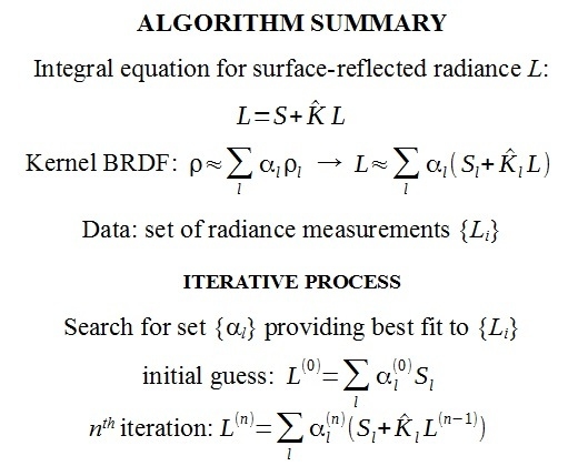
2.2. Iterative Fitting Algorithm to Derive BRDF from the Surface-Reflected Radiance

The fact that source function S Equation (2) of Equation (1) provides very good initial approximation of the reflected radiance $L(\mathsf{\tau }={\mathsf{\tau }}_t,-\mathsf{\mu },\mathsf{\varphi },{\mathsf{\mu }}_0)$ gives us an idea to improve that initial approximation by iterations. We will assume that the atmospheric state is known, i.e., radiances I and J can be modeled on their entire domains; and that real BRDF can be approximated by a finite set of kernels, see e.g., Lucht, et al, [17],

$$\mathsf{\rho }\left({\mathsf{\theta }}_s,{\mathsf{\theta }}_v,\mathsf{\varphi }\right) \approx {\displaystyle \sum _{l=1}^k{\mathsf{\alpha }}_l}{\mathsf{\rho }}_l\left({\mathsf{\theta }}_s,{\mathsf{\theta }}_v,\mathsf{\varphi }\right),$$

(4)

so that the problem is reduced to obtaining weights of the kernels ${\mathsf{\alpha }}_l$. We will also assume that BRDF ρ and kernels ρ_l are symmetric functions of relative azimuth φ. Then, substituting Equation (4) into Equations (1)–(3) we obtain

$$L(\mathsf{\tau }={\mathsf{\tau }}_t,-\mathsf{\mu },\mathsf{\varphi },{\mathsf{\mu }}_0)\approx {\displaystyle \sum _{l=1}^k{\mathsf{\alpha }}_l}\left\{S_l\left({\mathsf{\mu }}_0, \mathsf{\mu },\mathsf{\varphi }\right) + {\displaystyle \underset{0}{\overset{2\pi }{\int }}d{\mathsf{\varphi }}_2}{\displaystyle \underset{0}{\overset{1}{\int }}d{\mathsf{\mu }}_2{K}_l(\mathsf{\mu },{\mathsf{\mu }}_2,\mathsf{\varphi }-{\mathsf{\varphi }}_2)L(\mathsf{\tau }={\mathsf{\tau }}_t,-{\mathsf{\mu }}_2,{\mathsf{\varphi }}_2,{\mathsf{\mu }}_0)}\right\},$$

(5)

where

$$S_l\left({\mathsf{\mu }}_0, \mathsf{\mu },\mathsf{\varphi }\right) = I_0{\mathsf{\mu }}_0\exp \left({-\mathsf{\tau }}_t/{\mathsf{\mu }}_0\right){\mathsf{\rho }}_l\left({\mathsf{\mu }}_0, \mathsf{\mu },\mathsf{\varphi }\right) + {\displaystyle \underset{0}{\overset{2\pi }{\int }}d{\mathsf{\varphi }}_1}{\displaystyle \underset{0}{\overset{1}{\int }}d{\mathsf{\mu }}_1}{ \mathsf{\mu }}_1{\mathsf{\rho }}_l\left({\mathsf{\mu }}_1, \mathsf{\mu },\mathsf{\varphi }-{\mathsf{\varphi }}_1\right)I\left({\mathsf{\tau } = \mathsf{\tau }}_t{, \mathsf{\mu }}_1,{\mathsf{\varphi }}_1{, \mathsf{\mu }}_0\right),$$

(6)

$$K_l\left({\mathsf{\mu }, \mathsf{\mu }}_2,\mathsf{\varphi }-{\mathsf{\varphi }}_2\right) = {\displaystyle \underset{0}{\overset{2\pi }{\int }}d{\mathsf{\varphi }}_1}{\displaystyle \underset{0}{\overset{1}{\int }}d}{\mathsf{\mu }}_1{ \mathsf{\mu }}_1{\mathsf{\rho }}_l\left({\mathsf{\mu }}_1, \mathsf{\mu },\mathsf{\varphi }-{\mathsf{\varphi }}_1\right)J\left({\mathsf{\tau } = 0, -\mathsf{\mu }}_1,{\mathsf{\varphi }}_1-{\mathsf{\varphi }}_2{, \mathsf{\mu }}_2\right)/I_0,$$

(7)

Surface-reflected radiance L is usually measured on a limited set of sun-to-observer geometries, so we assume that L is known on a sparse set {μ_0,i, μ_i, φ_i}, i = 1, ... p. Then, the algorithm somewhat resembles the iterative process in Gatebe, et at. [23] and BRDF retrievals iterative process of MAIAC [24], see Equation (3) there. Equation (5) is used twice in every step: first to obtain an approximation of BRDF and second to improve current approximation of L.

0-th approximation:

Step A: minimal square fit to find coefficients $\left\{{\mathsf{\alpha }}_l^{(0)}\right\}$, l = 1, …, k, so that ${\displaystyle \sum _{l=1}^k{\mathsf{\alpha }}_l^{\left(0\right)}}{S}_l\left({\mathsf{\mu }}_0, \mathsf{\mu },\mathsf{\varphi }\right)$ is the best match to the set of experimental data $\left\{L_i\right\}=\left\{L(\mathsf{\tau }={\mathsf{\tau }}_t,-{\mathsf{\mu }}_i,{\mathsf{\varphi }}_i,{\mathsf{\mu }}_{0,i})\right\}$;

Step B: compute 0-th approximation of surface-reflected radiance as

$$L(\mathsf{\tau }={\mathsf{\tau }}_t,-\mathsf{\mu },\mathsf{\varphi },{\mathsf{\mu }}_0) = {\displaystyle \sum _{l=1}^k{\mathsf{\alpha }}_l^{\left(0\right)}}{S}_l\left({\mathsf{\mu }}_0, \mathsf{\mu },\mathsf{\varphi }\right).$$

(8)

at all values of its arguments needed for evaluation of the integral term in Equation (5);

First approximation:

Step A: minimal square fit to find coefficients $\left\{{\mathsf{\alpha }}_l^{(1)}\right\}$, l = 1, …, k, so that ${\displaystyle \sum _{l=1}^k{\mathsf{\alpha }}_l^{(1)}}\left\{S_l\left({\mathsf{\mu }}_0, \mathsf{\mu },\mathsf{\varphi }\right) + {\displaystyle \underset{0}{\overset{2\pi }{\int }}d{\mathsf{\varphi }}_2}{\displaystyle \underset{0}{\overset{1}{\int }}d{\mathsf{\mu }}_2{K}_l(\mathsf{\mu },{\mathsf{\mu }}_2,\mathsf{\varphi }-{\mathsf{\varphi }}_2)L^{(0)}(\mathsf{\tau }={\mathsf{\tau }}_t,-{\mathsf{\mu }}_2,{\mathsf{\varphi }}_2,{\mathsf{\mu }}_0)}\right\}$ is the best match to the set of experimental data $\left\{L_i\right\}$;

Step B: compute first approximation of surface-reflected radiance as

$$L^{(1)}(\mathsf{\tau }={\mathsf{\tau }}_t,-\mathsf{\mu },\mathsf{\varphi },{\mathsf{\mu }}_0)={\displaystyle \sum _{l=1}^k{\mathsf{\alpha }}_l^{(1)}}\left\{S_l\left({\mathsf{\mu }}_0, \mathsf{\mu },\mathsf{\varphi }\right) + {\displaystyle \underset{0}{\overset{2\pi }{\int }}d{\mathsf{\varphi }}_2}{\displaystyle \underset{0}{\overset{1}{\int }}d{\mathsf{\mu }}_2{K}_l(\mathsf{\mu },{\mathsf{\mu }}_2,\mathsf{\varphi }-{\mathsf{\varphi }}_2)L^{(0)}(\mathsf{\tau }={\mathsf{\tau }}_t,-{\mathsf{\mu }}_2,{\mathsf{\varphi }}_2,{\mathsf{\mu }}_0)}\right\},$$

(9)

at all values of its arguments needed to evaluate the integral term in Equation (5). The steps of the first approximation can be repeated until desirable convergence is reached.

2.3. Numerical Consideration

Due to the assumption that all quantities in the equations above are symmetric functions of azimuth, all integrations over interval [0, 2π] can be reduced to integration over interval [0, π]. This study employs the same quadrature scheme as used in Radkevich [14]: Gaussian rule {μ_j, β_j}, j = 1, …, m on [0, 1] and trapezoidal rule on a regular grid on [0, π] {φ_i, w_i}, i = 1, …, n, φ_i = Δφ(i − 1), w_i = Δφ(1 − δ_i,0/2 − δ_i,n/2), Δφ = π/(n − 1). Discretized Equation (1) takes the form

$$\begin{array}{cccc}{L}_{j,i}=S_{j,i} +{\displaystyle \sum _{s=1}^m{\displaystyle \sum _{l=1}^n{K}_{j,i,s,l}{L}_{s,l}}};& L_{j,i}=L(\mathsf{\tau }={\mathsf{\tau }}_t,-{\mathsf{\mu }}_j,{\mathsf{\varphi }}_i,{\mathsf{\mu }}_0);& i=1,\dots ,n;& j=1,\dots ,m;\end{array}$$

(10)

where

$$S_{j,i}=S({\mathsf{\mu }}_0,{\mathsf{\mu }}_j,{\mathsf{\varphi }}_i);$$

(11)

$$K_{j,i,s,l} = {\mathsf{\beta }}_j{w}_i\left(\left\{\begin{array}{c}K\left({\mathsf{\mu }}_j,{\mathsf{\mu }}_s,{\mathsf{\varphi }}_{i-l+1}\right), 1\le l\le i\\ K\left({\mathsf{\mu }}_j,{\mathsf{\mu }}_s,{\mathsf{\varphi }}_{l-i+1}\right), i+1\le l\le n\end{array}\right\} + \left\{\begin{array}{c}K\left({\mathsf{\mu }}_j,{\mathsf{\mu }}_s,{\mathsf{\varphi }}_{i+l-1}\right), 1\le l\le n-i+1\\ K\left({\mathsf{\mu }}_j,{\mathsf{\mu }}_s,{\mathsf{\varphi }}_{2n-i-l+1}\right), n-i+2\le l\le n\end{array}\right\}\right),$$

(12)

Numerical tests of the performance of the suggested algorithm were conducted with the following atmospheric conditions: the atmosphere is a uniform layer comprised of (a) Rayleigh scattering and weak gas absorption, so that single scattering albedo (SSA) is 0.999 and optical thickness τ_R of 0.1 (this roughly corresponds to the wavelength of 550 nm) and (b) transported mineral dust aerosol from OPAC [25] with optical thicknesses τ_A of 0.1, 0.5, and 1.0. Therefore, simplified atmospheric conditions are defined with Rayleigh scattering, aerosol scattering and absorption of a known aerosol type, and weak gas absorption. Single scattering properties of aerosol were computed with code SPHER [26]. It was found that it is essential to retain 138 terms in Legendre expansion of the phase function of the selected type of aerosol. Radiances L, I, J were computed with DISORT using 158 streams for all μ₀ and μ being nodes of the Gaussian quadrature of order m = 24 and φ on the regular grid described above with n = 49.

Surface-reflected radiance was computed for two BRDF models. First, bare soil model by Nilson and Kuusk [27], see Equations (11) and (11′) there

$$\begin{array}{c}\mathsf{\rho }\left({\mathsf{\theta }}_s,{\mathsf{\theta }}_v,\mathsf{\varphi }\right) = a\left(b_0 + b_1{\mathsf{\theta }}_s{\mathsf{\theta }}_v\cos \mathsf{\varphi }+b_2\left({\mathsf{\theta }}_s^2+{\mathsf{\theta }}_v^2\right) + b_3{\mathsf{\theta }}_s^2{\mathsf{\theta }}_v^2\right)\\ \begin{array}{ccccc}a=\underset{{\mathsf{\theta }}_s\to \mathsf{\pi }/2}{{\displaystyle \lim }}a\left({\mathsf{\theta }}_s\right)=0.2;& b_0=0.31489;& b_1=0.14129;& b_2=-0.082511;& b_3=0.14779\end{array}\end{array},$$

(13)

The second model is MODIS BRDF, see Equations (37)–(44) [17]

$$\mathsf{\rho }\left({\mathsf{\theta }}_s,{\mathsf{\theta }}_v,\mathsf{\varphi }\right) =\frac{1}{\mathsf{\pi }} \left(f_{iso}+f_{vol}{K}_{vol}({\mathsf{\theta }}_s,{\mathsf{\theta }}_v,\mathsf{\varphi })+f_{geo}{K}_{geo}({\mathsf{\theta }}_s,{\mathsf{\theta }}_v,\mathsf{\varphi })\right),$$

(14)

where factor 1/π comes in due to the difference in definitions, so that we will denote α₁ = f_iso/π, α₂ = f_vol/π, α₃ = f_geo/π. In this study, the following particular values of the parameters were used: f_iso = 0.265, f_vol = 0.066, f_geo = 0.000 (α₁ = 0.08435, α₂ = 0.02101, α₃ = 0.0000) representing actual MODIS BRDF retrievals [28] over the Sahara Desert.

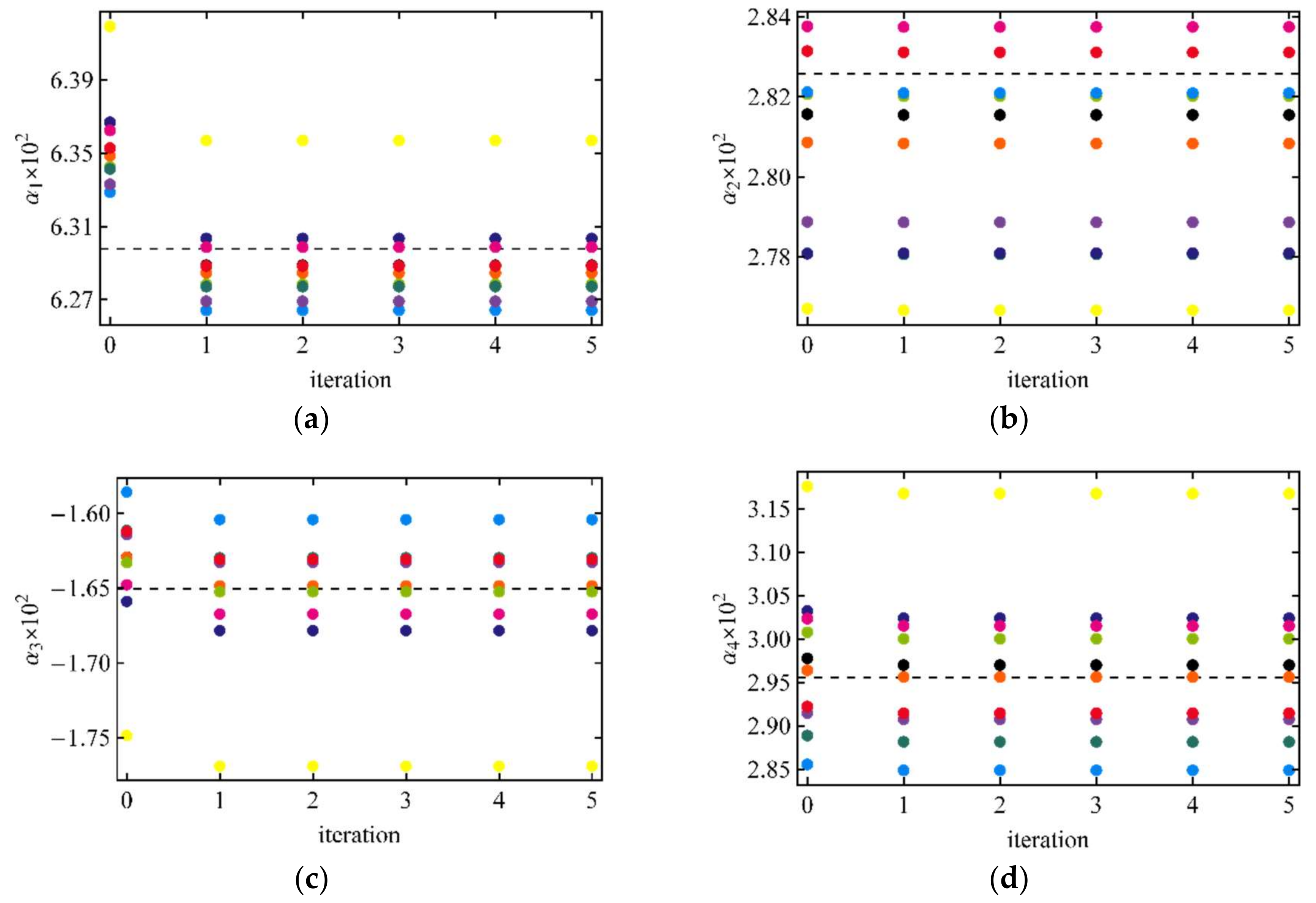
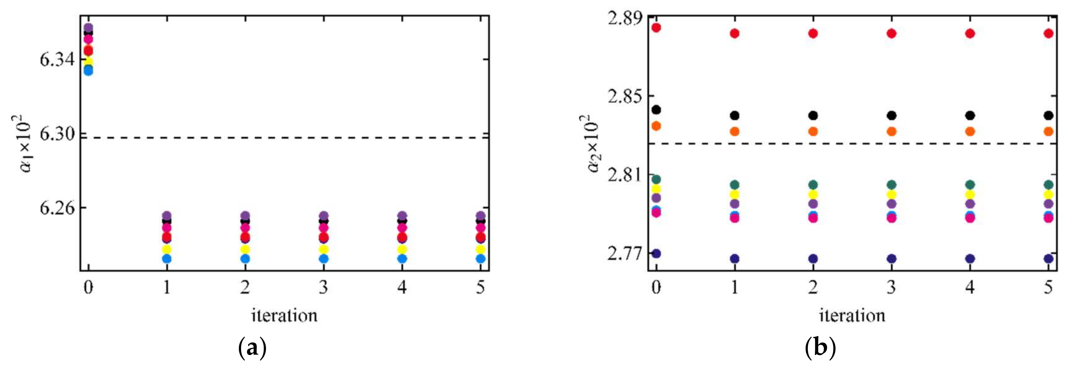
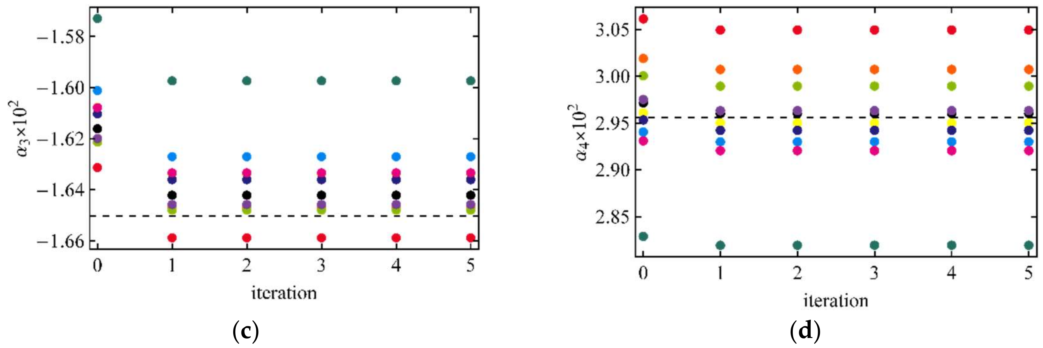
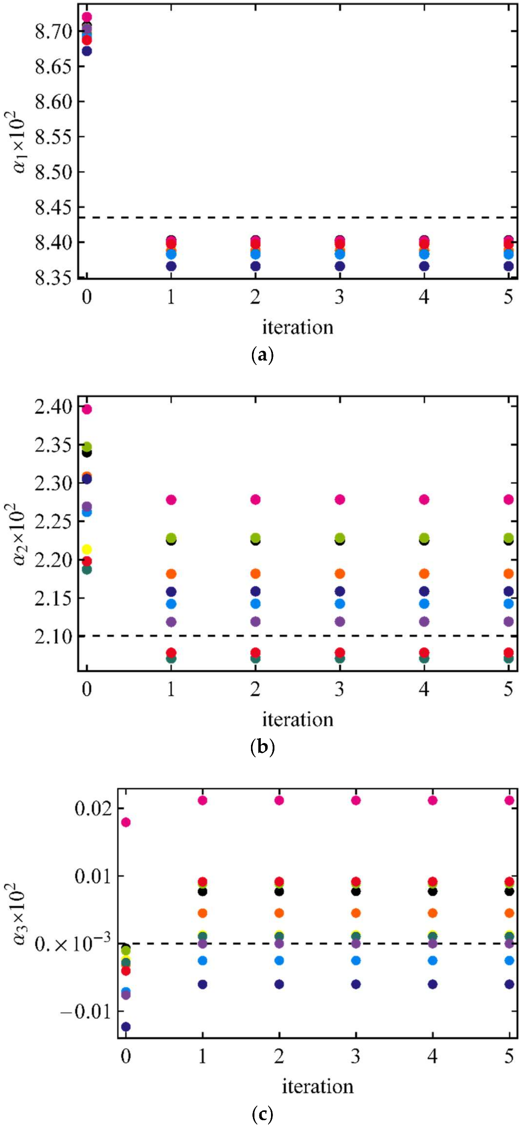
3. Results of BRDF Retrievals

Surface-reflected radiance L, obtained by solving the boundary value problem to the radiative transfer equation with DISORT, can be used as a simulation of experimental measurements if taken at sparse geometries. Paper [14] compares radiance L directly computed with DISORT with numerical solution of Equation (1) using radiance I and J also computed with DISORT. It was found that the solution obtained with DISORT has noticeable azimuthal noise of the order of few percent, see Figure 1, Figure 2 and Figure 3 there. The numerical solution of Equation (1) obtained in Radkevich [14] is not independent from errors introduced by DISORT, thus it cannot be considered as more accurate. Though the origin of this noise is beyond the scope of this paper, its presence in the solution makes it a valuable opportunity to check robustness of BRDF retrievals by the iterative process described above.

Numerical experiments below will use surface-reflected radiance L computed on the grid described in Section 2.3. Random selections of 12 and 60 geometries, i.e., values of {μ_0,i, μ_i, φ_i}, were performed for each optical thickness, so that retrievals were performed on different sets of data. The purpose of this study is to test the developed algorithm, so the optimized selection of data samples suggested in study [29] was not used. The final results of retrievals are summarized in

Table 1. Parameters of Nilson–Kuusk BRDF, Equation (13), retrieved from surface radiance using 10 sets of 60 (a), and 10 sets of 12 (b) randomly selected sun-to-sensor geometries for different optical thickness of the atmosphere multiplied by 100.

		τt = 0.2: τR = 0.1, τA = 0.1		τt = 0.6: τR = 0.1, τA = 0.5		τt = 1.1: τR = 0.1, τA = 1.0
Parameter	Theoretical Value	Mean Value	Standard Deviation	Mean Value	Standard Deviation	Mean Value	Standard Deviation
(a)
α1	6.298	6.286	0.004	6.260	0.015	6.243	0.008
α2	2.826	2.815	0.008	2.793	0.027	2.809	0.033
α3	−1.650	−1.646	0.004	−1.645	0.019	−1.637	0.017
α4	2.956	2.948	0.013	2.964	0.055	2.953	0.061
(b)
α1	6.298	6.291	0.026	6.256	0.109	6.193	0.325
α2	2.826	2.805	0.024	2.866	0.141	2.770	0.160
α3	−1.650	−1.656	0.045	−1.622	0.195	−1.564	0.314
α4	2.956	2.968	0.091	2.933	0.297	2.860	0.323

and

Table 2. Parameters of MODIS BRDF, Equation (14), retrieved from surface radiance using 10 sets of 60 (a), and 10 sets of 12 (b) randomly selected sun-to-sensor geometries for different optical thickness of the atmosphere multiplied by 100.

		τt = 0.6: τR = 0.1, τA = 0.5		τt = 1.1: τR = 0.1, τA = 1.0
Parameter	Theoretical Value	Mean Value	Standard Deviation	Mean Value	Standard Deviation
(a)
α1	8.435	8.392	0.012	8.373	0.016
α2	2.101	2.156	0.072	2.099	0.058
α3	0.	0.005	0.008	−0.001	0.005
(b)
α1	8.435	8.348	0.079	8.404	0.086
α2	2.101	2.163	0.171	2.187	0.146
α3	0.	−0.026	0.060	0.012	0.043

. The iterative process of retrievals are shown in Figure 1, Figure 2 and Figure 3. As one can see from the figure’s zeroth iteration, Equation (8) provides good accuracy but it can be improved with the first iteration, Equation (9). The difference between first and second iterations can be hardly seen on the graphs. Within an accuracy of seven decimal figures, there is no difference between the second and all subsequent iterations. Therefore, for practical purposes zeroth and first iterations are enough for the process to converge.

Table 1a,b show that the increase of the aerosol optical thickness from 0.1 to 0.5 causes the increase of the standard deviation ${\mathsf{\sigma }}_l$ of the retrieved parameters ${\mathsf{\alpha }}_l$ while further increase of τ_A to 1.0 does not cause the same effect. Table 2a,b also show no clear tendency for ${\mathsf{\sigma }}_l$ in this case. Also, greater τ_A (and, consequently, greater τ_t) leads to greater difference between ${\overline{\mathsf{\alpha }}}_l$ and theoretical values ${\mathsf{\alpha }}_{t,l}$ in some cases. However, theoretical values ${\mathsf{\alpha }}_{t,l}$ either falls into 1-σ confidence interval around the mean values ${\overline{\mathsf{\alpha }}}_l$ or the relative difference between ${\overline{\mathsf{\alpha }}}_l$ and ${\mathsf{\alpha }}_{t,l}$ does not exceed 2%.

4. Discussion

Analysis of Table 1 and Table 2 shows that mean values over 10 randomly selected sun-to-sensor geometries are closer to theoretical values for optically thin atmosphere. It means that even in the ideal case of modeling surface signals with known BRDF and atmospheric conditions, the accuracy of the radiative transfer modeling affects the accuracy of BRDF retrievals. The problem here is at least two-fold. First, the noise in surface-reflected radiance increases with the increase of the optical thickness, making retrievals from it less accurate. Second, since the retrieval process depends on the radiances I and J transmitted through and reflected by unbound atmosphere, their accuracy and potential presence of noise also affect the accuracy of the retrieval process.

The iterative process itself shows very quick convergence regardless of the surface type and atmospheric conditions.

The accuracy of the retrievals under different atmospheric conditions and for different surfaces can be illustrated with 1-σ confidence intervals relative to the theoretical value for those parameters which have non-zero α_t,l

$${\mathsf{\epsilon }}_{\pm }=[(|{\overline{\mathsf{\alpha }}}_l|\pm {\mathsf{\sigma }}_l)/|{\mathsf{\alpha }}_{t,l}|-1]\times 100\%,$$

(15)

These relative intervals are presented in

Table 3. Relative confidence intervals, Equation (15), of the retrieved parameters of Nilson–Kuusk BRDF, Equation (13), retrieved from surface radiance using 10 sets of 60 (a), and 10 sets of 12 (b) randomly selected sun-to-sensor geometries for different optical thickness of the atmosphere.

	τt = 0.2: τR = 0.1, τA = 0.1		τt = 0.6: τR = 0.1, τA = 0.5		τt = 1.1: τR = 0.1, τA = 1.0
	${\mathsf{\epsilon }}_{-}$	${\mathsf{\epsilon }}_{+}$	${\mathsf{\epsilon }}_{-}$	${\mathsf{\epsilon }}_{+}$	${\mathsf{\epsilon }}_{-}$	${\mathsf{\epsilon }}_{+}$
(a)
α1	−0.25	−0.13	−0.84	−0.37	−1.00	−0.75
α2	−0.67	−0.11	−2.12	−0.21	−1.77	0.57
α3	−0.48	0.00	−1.45	0.85	−1.82	0.24
α4	−0.71	0.17	−1.59	2.13	−2.17	1.96
(b)
α1	−0.52	0.30	−2.40	1.06	−6.83	3.49
α2	−1.59	0.11	−3.57	6.40	−7.64	3.68
α3	−2.36	3.09	−13.52	10.12	−24.24	13.82
α4	−2.67	3.48	−10.83	9.27	−14.17	7.68

and

Table 4. Relative confidence intervals, Equation (15), of the retrieved parameters of MODIS BRDF, Equation (14), retrieved from surface radiance using 10 sets of 60 (a), and 10 sets of 12 (b) randomly selected sun-to-sensor geometries for different optical thickness of the atmosphere.

	τt = 0.6: τR = 0.1, τA = 0.5		τt = 1.1: τR = 0.1, τA = 1.0
	${\mathsf{\epsilon }}_{-}$	${\mathsf{\epsilon }}_{+}$	${\mathsf{\epsilon }}_{-}$	${\mathsf{\epsilon }}_{+}$
(a)
α1	−0.65	−0.37	−0.92	−0.55
α2	−0.81	6.04	−2.86	2.67
(b)
α1	−1.97	−0.09	−1.39	0.65
α2	−5.19	11.09	−2.86	11.04

below.

Confidence intervals are generally smaller for smaller optical thicknesses and for the greater number of ‘observations’ used in the retrieval process. It is easy to see that, in many instances, one parameter has positive bias while another has negative. This leads to some cancellation of errors, reducing the overall error in albedo.

It is important to mention that for MODIS BRDF (Equation (14)) retrieval testing one of the parameters, α₃, was deliberately chosen to be zero. The purpose was to check how accurately this zero can be caught by the retrieval algorithm. Lucht and co-authors [17] argued that retrieved parameters of BRDF (Equation (14)) should be non-negative. Lewis [16], considering retrievals of the kernel weight with minimization of the error function, argued that “the minimum of the error function described above can sometimes lie outside of physical limits. In this case, the minimum lies on one of the constraint boundaries in N_k-dimensional space.” (N_k is the number of kernels, k in notation of this paper). Following this idea, study [17] suggests that “if the mathematical inversion produces a negative parameter, the next best valid value for this parameter is zero, under which imposed condition, the remaining kernel parameters should be re-derived.” In the case presented in Figure 3c, all retrievals are wrong, both positive and negative. There are three negative and seven positive retrievals there. Following the approach above, negative values should be set to zero and the retrieval algorithm should be re-run without a third kernel while sevrn positive but equally wrong values should be left as is. The approach can be modified in this situation. If an algorithm is intended to be used on a certain amount of data points of certain quality, then performance (absolute error δ_l of each parameter) of the retrievals can be established statistically with extensive radiative transfer modeling. Then, if a retrieved value α_l falls into an interval α_m,l ± δ_l around its marginal value α_m,l, α_l should be set α_m,l. In the case shown in Figure 3c α_m,3 = 0.0, δ₃ can be set—e.g., equal σ₃ = 0.008—see the corresponding value in Table 2a. This eliminates four (out of seven) positive values of α₃. Setting δ₃ = 2σ₃ eliminates six and δ₃ = 3σ₃ eliminates all seven positive (and wrong) retrievals of α₃.

5. Conclusions

An algorithm for retrievals of BRDF from the surface-reflected radiance measured at the ground level is presented. The algorithm is based on the equation relating BRDF with the surface-reflected radiance and the solutions of the RT problems for unbound atmosphere. The previous analysis of the contributions of the different terms of the equation for the reflected radiance suggested that only minor correction to the source term of the equation has to be done. Therefore, fast convergence of the iterative process could be expected.

The presented algorithm requires an assumption on the atmospheric condition. It is based on kernel-based BRDF; therefore, it also requires an assumption on the functional form of the kernels comprising BRDF. The algorithm returns the weights of the kernels. The choice of the kernels depends on the physical properties of the surface. A potential application of the algorithm is derivation of BRDF parameter from measurements acquired in ground-based experimental campaigns. It is desirable to have measurements performed simultaneously with sun-photometer measurements similar to AERONET [30] to ensure accurate retrieval of aerosol properties.

It was shown that the algorithm converges very quickly; no more than one iteration (after initial guess) is needed. Accuracy of the algorithm depends on the number of experimental measurements used for retrievals, optical thickness of the atmosphere, and the quality of the measurements of the surface-reflected radiance. The last two factors may not be independent in the context of this study since the surface-reflected radiance was simulated with DISORT. It was shown in a previous study [14] that there is some noise in those simulations with magnitude increasing with the optical thickness of the atmosphere. Retrievals were performed on the sets of 12 and 60 randomly selected sun-to-sensor geometries. While the mean values of the retrieved kernel weights over 10 sets of geometries are within ~5% of the theoretical values for both 12 and 60 samples (with better matches for optically thinner cases), the range on those sets are wider for the smaller number reaching up to ~25% in certain cases, but staying generally within ~10%.

References

1. Meister, G.; Wiemker, R.; Bienlein, J. In Situ BRDF Measurements of Selected Surface Materials to Improve Analysis of Remotely Sensed Multispectral Imagery. ISPRS Arch. 1996, 31 Pt B7, 493–498. [Google Scholar]
2. Deering, D.W.; Eck, T.F.; Grier, T. Shinnery Oak Bidirectional Reflectance Properties and Canopy Model Inversion. IEEE Trans. Geosci. Remote Sens. 1992, 30, 339–348. [Google Scholar] [CrossRef]
3. Leroux, C.; Deuzé, J.-L.; Goloub, P.; Sergent, C.; Fily, M. Ground measurements of the polarized bidirectional reflectance of snow in the near-infrared spectral domain: Comparison with model results. J. Geophys. Res. 1998, 103, 19721–19731. [Google Scholar] [CrossRef]
4. Hudson, S.R.; Warren, S.G.; Brandt, R.E.; Grenfell, T.C.; Six, D. Spectral bidirectional reflectance of Antarctic snow: Measurements and parameterization. J. Geophys. Res. 2006, 111, D18106. [Google Scholar] [CrossRef]
5. Huang, X.; Jiao, Z.; Dong, Y.; Zhang, H.; Li, X. Analysis of BRDF and Albedo Retrieved by Kernel-Driven Models Using Field Measurements. IEEE J. Sel. Top. Appl. Earth Obs. Remote Sens. 2013, 6, 149–161. [Google Scholar] [CrossRef]
6. Chopping, M.J. Testing a LiSK BRDF Model with in Situ Bidirectional Reflectance Factor Measurements over Semiarid Grasslands. Remote Sens. Environ. 2000, 74, 287–312. [Google Scholar] [CrossRef]
7. Walthall, C.; Roujean, J.-L.; Morisette, J. Field and landscape BRDF optical wavelength measurements: Experience, techniques and the future. Remote Sens. Rev. 2000, 18, 503–531. [Google Scholar] [CrossRef]
8. Bruegge, C.; Helmlinger, M.; Conel, J.; Gaitley, B.; Abdou, W. PARABOLA III—A sphere-scanning radiometer for field determination of surface anisotropic reflectance functions. Remote Sens. Rev. 2000, 19, 75–94. [Google Scholar] [CrossRef]
9. Martonchik, J.V. Retrieval of surface directional reflectance properties using ground level multiangle measurements. Remote Sens. Environ. 1994, 50, 303–316. [Google Scholar] [CrossRef]
10. Lyapustin, A.I.; Privette, J.L. A new method of retrieving surface bidirectional reflectance from ground measurements: Atmospheric sensitivity study. J. Geophys Res. 1999, 104, 6257–6268. [Google Scholar] [CrossRef]
11. Lyapustin, A.I.; Knyazikhin, Y. Green’s function method for the radiative transfer problem. I. Homogeneous non-Lambertian surface. Appl. Opt. 2001, 40, 3495–3501. [Google Scholar] [CrossRef] [PubMed]
12. Lyapustin, A.; Martonchik, J.; Wang, Y.; Laszlo, I.; Korkin, S. Multi-Angle Implementation of Atmospheric Correction (MAIAC): Part 1. Radiative Transfer Basis and Look-Up Tables. J. Geophys. Res. 2011, 116, D03210. [Google Scholar] [CrossRef]
13. Radkevich, A. A new look at decoupling of atmospheric radiative transfer and anisotropic surface reflection. JQSRT 2013, 127, 140–148. [Google Scholar] [CrossRef]
14. Radkevich, A. Iterative discrete ordinates solution of the equation for surface-reflected radiance. JQSRT 2017, 202, 114–125. [Google Scholar] [CrossRef]
15. Roujean, J.-L.; Leroy, M.; Deschamps, P.Y. A bidirectional reflectance model of the Earth’s surface for the correction of remote sensing data. J. Geophys. Res. 1992, 97, 20455–20468. [Google Scholar] [CrossRef]
16. Lewis, P. The utility of kernel-driven BRDF models in global BRDF and albedo studies. In Proceedings of the Geoscience and Remote Sensing Symposium, Firenze, Italy, 10–14 July 1995. [Google Scholar] [CrossRef]
17. Lucht, W.; Schaaf, C.B.; Strahler, A.H. An algorithm for the retrieval of albedo from space using semiempirical BRDF models. IEEE Trans. Geosci. Remote Sens. 2000, 38, 977–998. [Google Scholar] [CrossRef]
18. Pokrovsky, O.; Roujean, J.-L. Land surface albedo retrieval via kernel-based BRDF modeling: I. Statistical inversion method and model comparison. Remote Sens. Environ. 2002, 84, 100–119. [Google Scholar] [CrossRef]
19. Gao, F.; Schaaf, C.B.; Strahler, A.H.; Jin, Y.; Li, X. Detecting vegetation structure using a kernel-based BRDF model. Remote Sens. Environ. 2003, 86, 198–205. [Google Scholar] [CrossRef]
20. Román, M.O.; Gatebe, C.K.; Schaaf, C.B.; Poudyal, R.; Wang, Z.; King, M.D. Variability in surface BRDF at different spatial scales (30 m–500 m) over a mixed agricultural landscape as retrieved from airborne and satellite spectral measurements. Remote Sens. Environ. 2011, 115, 2184–2203. [Google Scholar] [CrossRef]
21. Liu, S.; Liu, Q.; Liu, Q.; Wen, J.; Li, X. The Angular and Spectral Kernel Model for BRDF and Albedo Retrieval. IEEE J. Sel. Top. Appl. Earth Obs. Remote Sens. 2010, 3, 242–256. [Google Scholar] [CrossRef]
22. Roujean, J.-L. Inversion of Lumped Parameters Using BRDF Kernels. Compre Remote Sens. 2018, 3, 23–34. [Google Scholar] [CrossRef]
23. Gatebe, C.K.; King, M.D.; Lyapustin, A.I.; Arnold, G.T.; Redemann, J. Airborne Spectral Measurements of Ocean Directional Reflectance. J. Atmos. Sci. 2005, 62, 1072–1092. [Google Scholar] [CrossRef]
24. Lyapustin, A.I.; Wang, Y.; Laszlo, I.; Hilker, T.; Hall, F.G.; Sellers, P.J.; Tucker, C.J.; Korkin, S.V. Multi-angle implementation of atmospheric correction for MODIS (MAIAC): 3. Atmospheric correction. Remote Sens. Environ. 2012, 127, 385–393. [Google Scholar] [CrossRef]
25. Hess, M.; Koepke, P.; Schult, I. Optical Properties of Aerosols and Clouds: The Software Package OPAC. BAMS 1998, 79, 831–844. [Google Scholar] [CrossRef]
26. Mishchenko, M.I.; Travis, L.D.; Lacis, A.A. Scattering, Absorption, and Emission of Light by Small Particles; Cambridge University Press: Cambridge, UK, 2002; 448p, ISBN 9780521782524. [Google Scholar]
27. Nilson, T.; Kuusk, A. A reflectance model for the homogeneous plant canopy and its inversion. Remote Sens. Environ. 1989, 27, 157–167. [Google Scholar] [CrossRef]
28. Schaaf, C.B.; Gao, F.; Strahler, A.H.; Lucht, W.; Li, X.; Tsang, T.; Strugnell, N.C.; Zhang, X.; Jin, Y.; Muller, J.-P.; et al. First Operational BRDF, Albedo and Nadir Reflectance Products from MODIS. Remote Sens. Environ. 2002, 83, 135–148. [Google Scholar] [CrossRef]
29. Pokrovsky, O.; Roujean, J.-L. Land surface albedo retrieval via kernel-based BRDF modeling: II. An optimal design scheme for the angular sampling. Remote Sens. Environ. 2002, 84, 120–142. [Google Scholar] [CrossRef]
30. Holben, B.N.; Eck, T.F.; Slutsker, I.; Tanre, D.; Buis, J.P.; Setzer, A.; Vermote, E.; Reagan, J.A.; Kaufman, Y.; Nakajima, T.; et al. AERONET—A federated instrument network and data archive for aerosol characterization. Remote Sens. Environ. 1998, 66, 1–16. [Google Scholar] [CrossRef]
Figure 1. Convergence of coefficients αl (×100) in the case of BRDF (Equation (13)) with τR = 0.1, τR = 0.1. Different colors are 10 random realizations of 12 observations. Dashed lines—theoretical values. (a) α1; (b) α2; (c) α3; (d) α4.
Remotesensing 10 00591 g001
Figure 2. The same as Figure 1 but with τA = 1.0 and for 10 random realizations of 60 observations. (a) α1; (b) α2; (c) α3; (d) α4.
Remotesensing 10 00591 g002aRemotesensing 10 00591 g002b
Figure 3. Convergence of coefficients αl (×100) in the case of BRDF (Equation (14)) with τR = 0.1, τR = 0.5. Different colors are 10 random realizations of 60 observations. Dashed lines—theoretical values. (a) α1; (b) α2; (c) α3.
Remotesensing 10 00591 g003