An Efficient Parallel Multi-Scale Segmentation Method for Remote Sensing Imagery

 ,
,  and
and
Abstract
:
1. Introduction
2. Multi-Scale Segmentation Method Based on MST and MHR
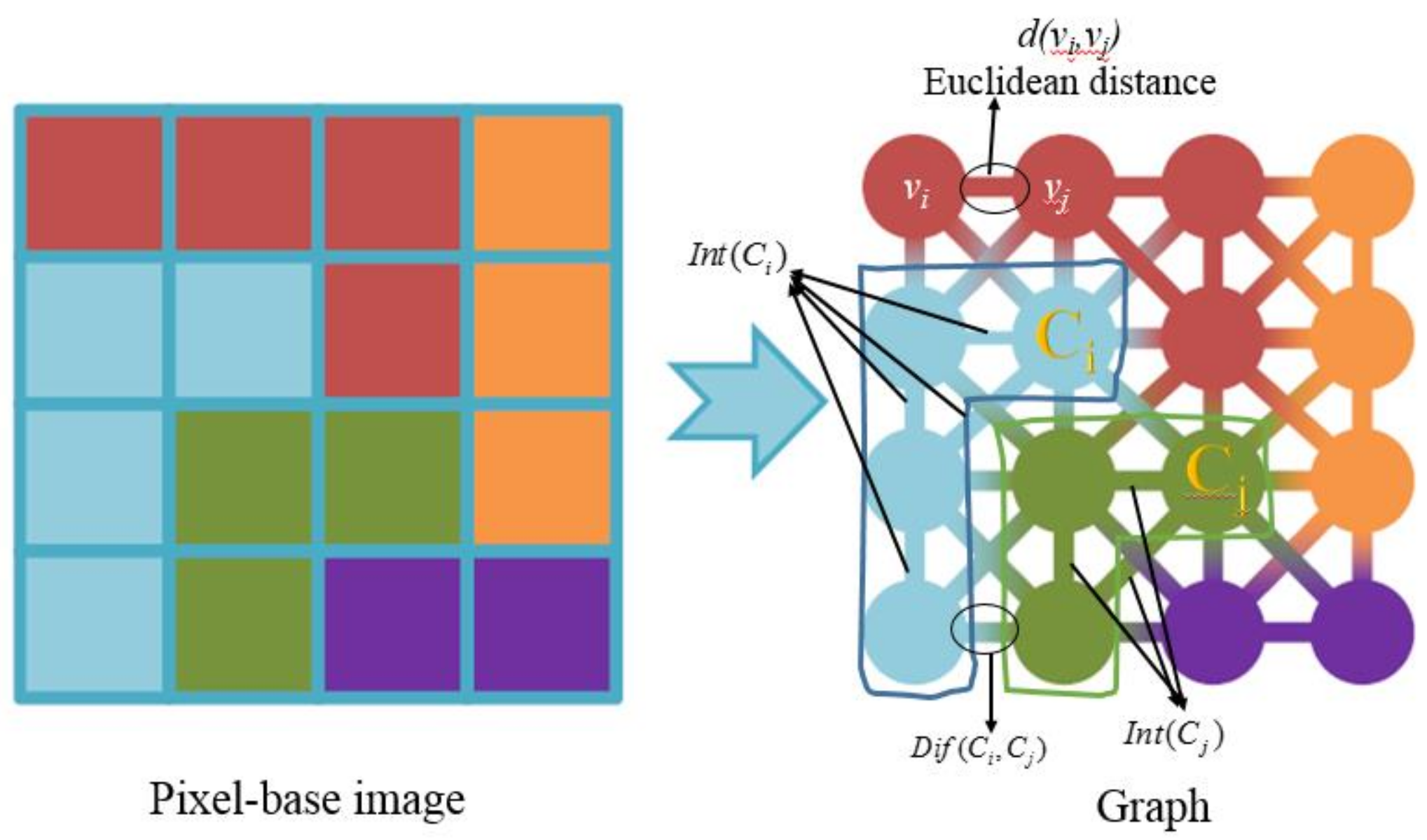
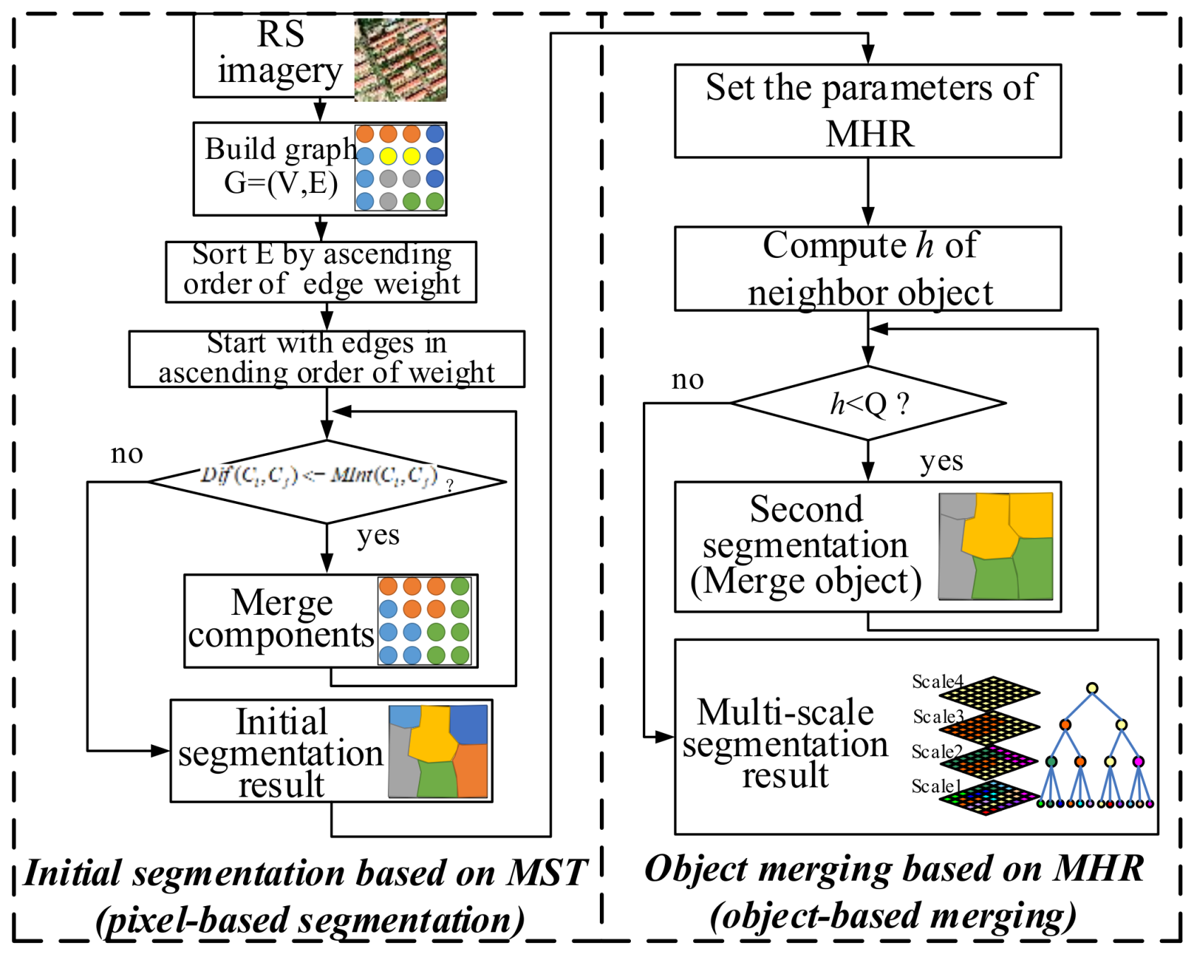
2.1. Initial Segmentation Based on MST
- (1)
- A graph with vertices V and edges E is built and the weight of each edge is the Euclidean distance between neighboring elements and in terms of the intensities of all the bands.
- (2)
- Sort E by non-decreasing edge weight.
- (3)
- Start with an initial segmentation S0, where each vertex is in its own component. Compute a threshold function for each component using Formula (5). Then Compute and for each component using Formulas (2) and (4). Subsequently we decide whether . If the condition holds, the two components are merged; otherwise nothing would be done. Repeat the above steps until all the components are computed.
- (4)
- The output is a segmentation of V into components .
2.2. Object Merging Based on MHR
- (1)
- Set the parameters of MHR, such as weights of color, shape, compact, and smooth (, , , ), and the scale parameter Q. Then compute the heterogeneity h of adjacent objects using Formula (6).
- (2)
- Decide whether h satisfies MHR. If h < (Q)2, the adjacent smaller objects are merged into a bigger one. Meanwhile, the average size, standard deviation, and mean of all the objects are calculated. Repeat this process until all the objects are merged.
- (3)
- Repeat steps 1–2 to accomplish the multi-scale segmentations.
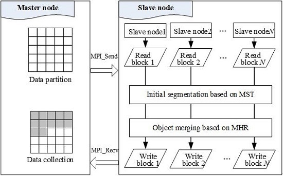
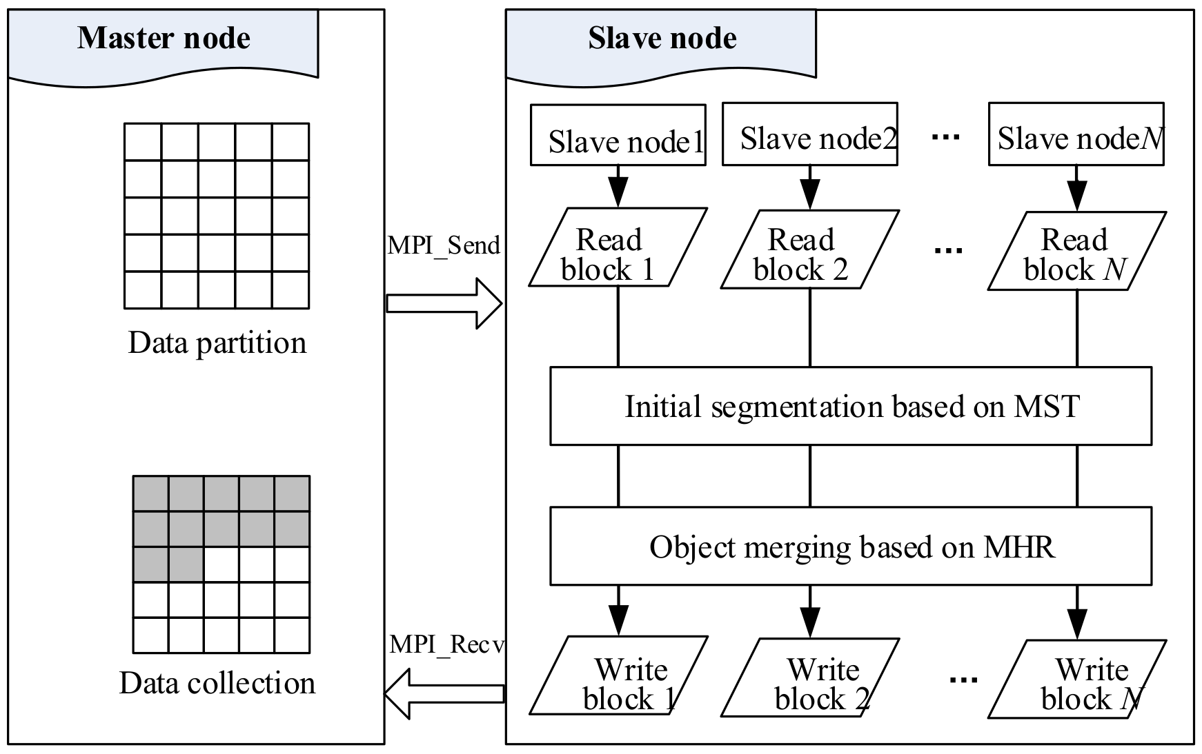
3. Parallel Segmentation Based on MPI
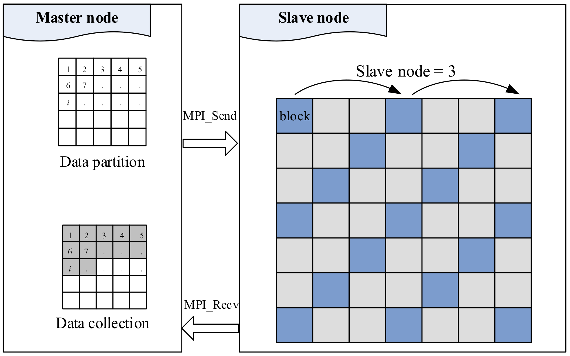
3.1. Data Partition Strategy
- (1)
- The data is divided into rectangular blocks, and every block is labelled with “1, 2, 3, …, i, …” from left to right, up to down.
- (2)
- Each block is assigned to a different slave node; the block is labelled as i, that is,where, (n, p) is the coordinate of the slave node, which is labeled with index i, and P is the number of slave nodes in the column direction. Here the column and row directions are equivalent to the coordinate in the x and y directions, respectively.
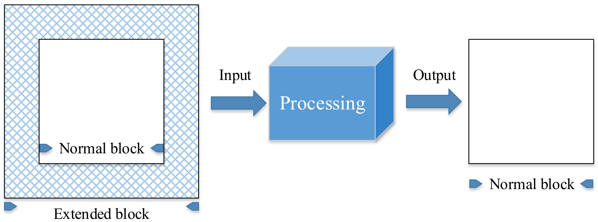
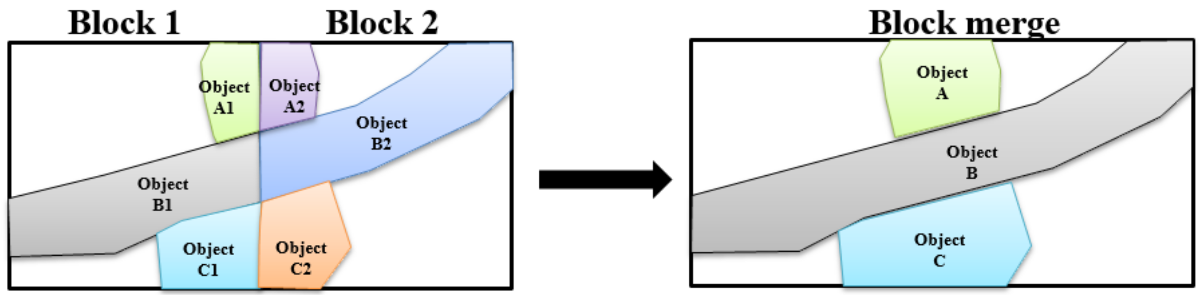
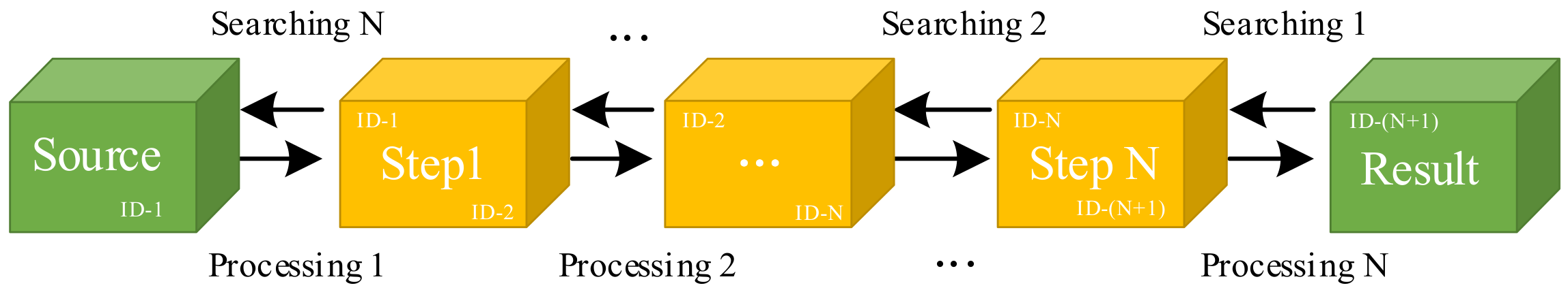
3.2. “Reverse Searching-Forward Processing” Chain
3.3. Parallel Segmentation Method
- (1)
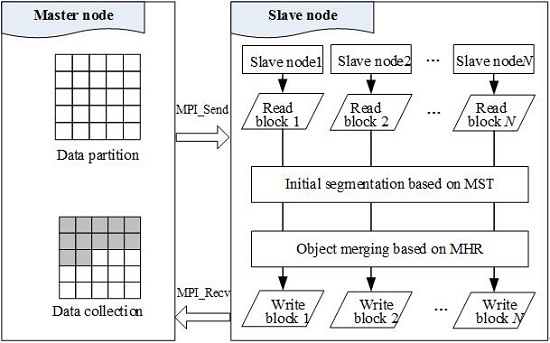
- The master node is responsible for reading the image and dividing it into blocks using extended buffer strategy. A regular data division is used to divide the original image data into sub-rectangular data blocks, which will be used as the input data and assigned to the slave nodes for parallel computing.
- (2)
- The slave nodes are responsible for receiving blocks. First, each block is segmented separately, and the data block is segmented to obtain objects initially based on MST. Then, the objects are merged based on MHR to obtain the results. In the end, all the segmentation results are sent to the master node.
- (3)
- The master node collects the results from each slave node, and outputs the segmentation image.
4. Test Sites and Experiments
4.1. Test Sites
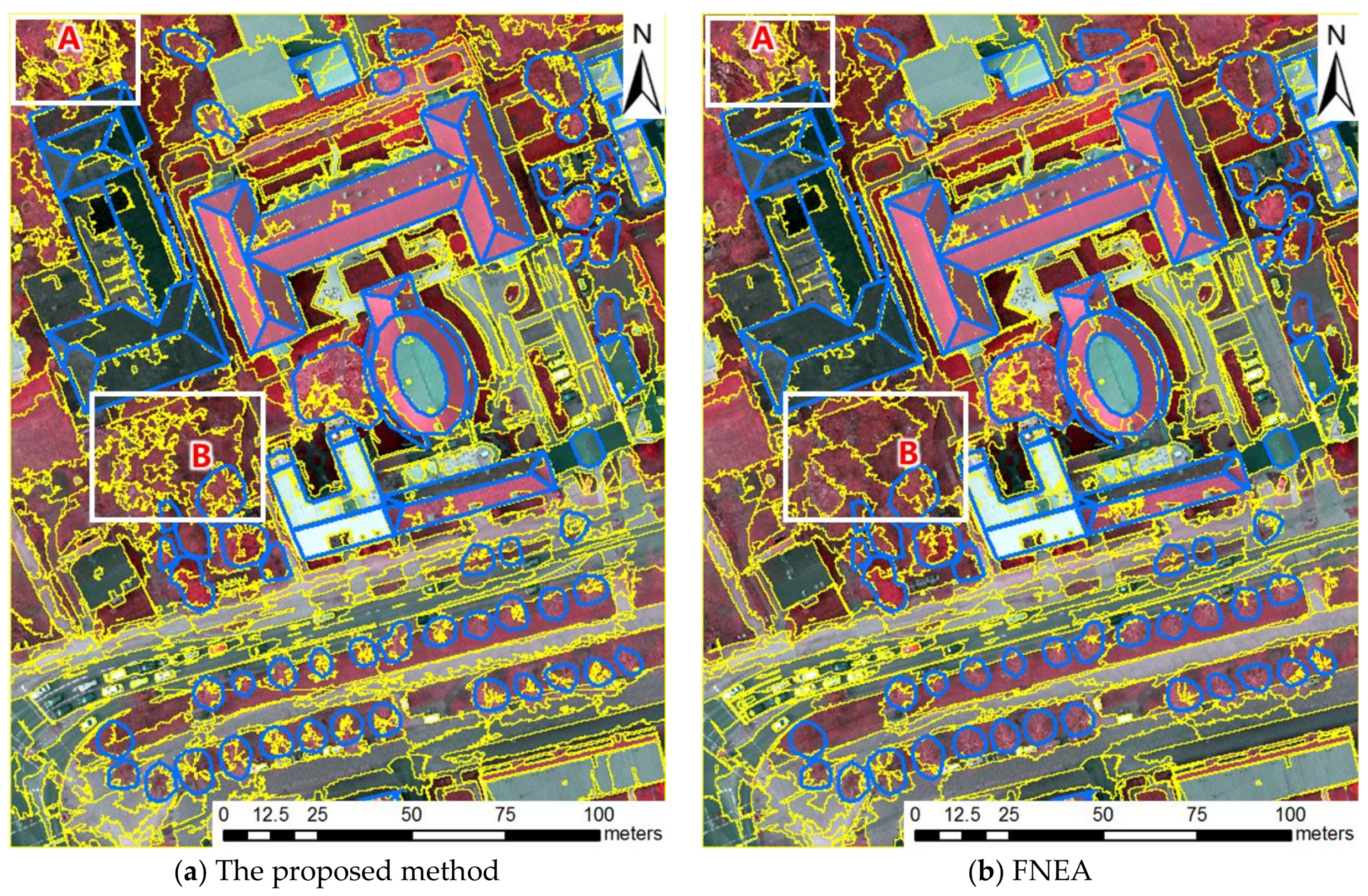
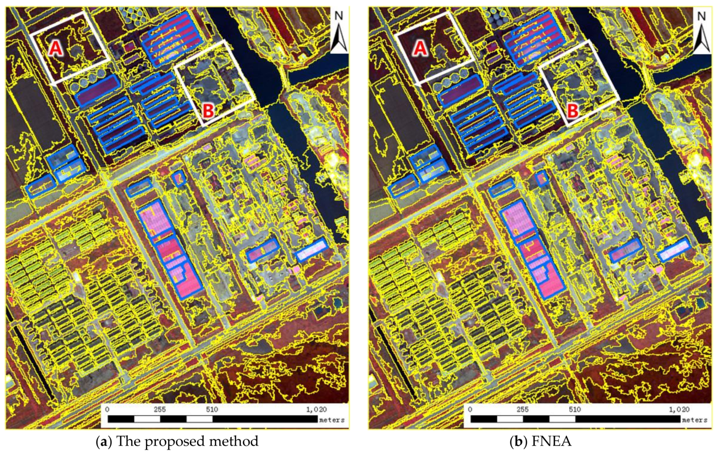
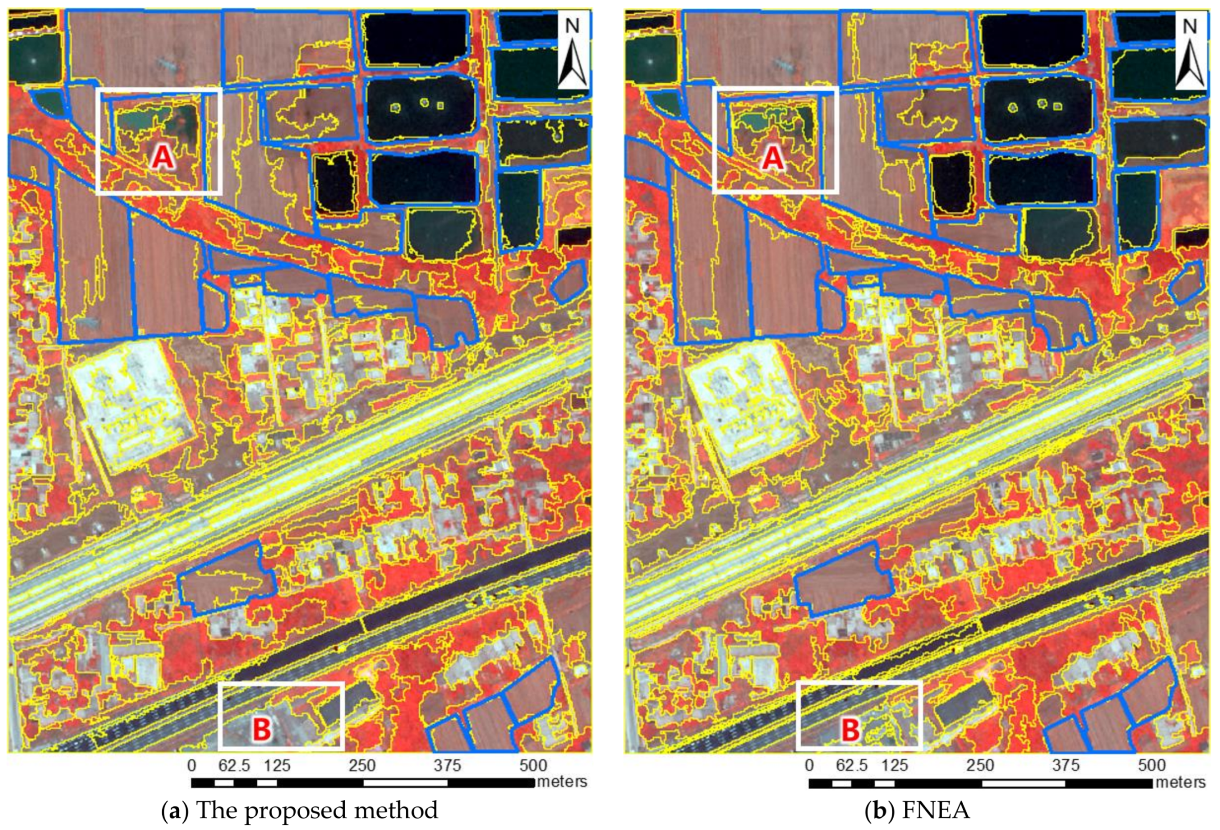
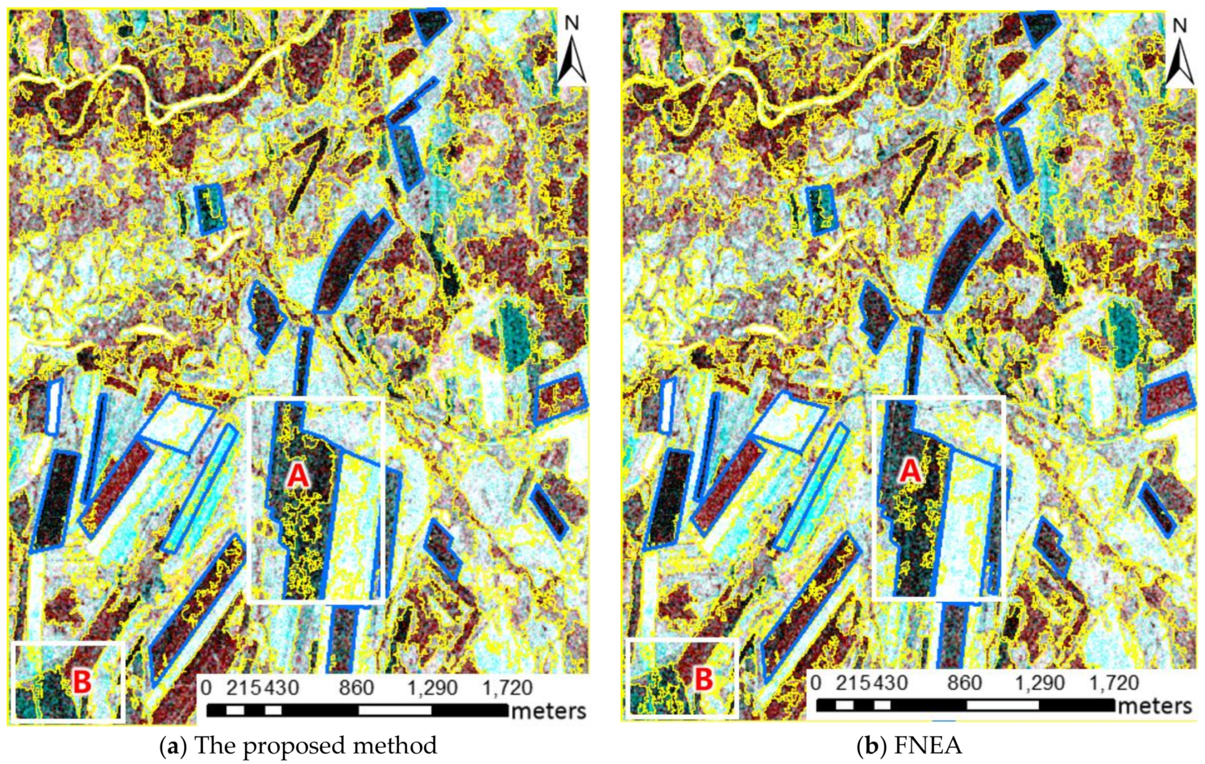
4.2. Results
4.3. Analysis
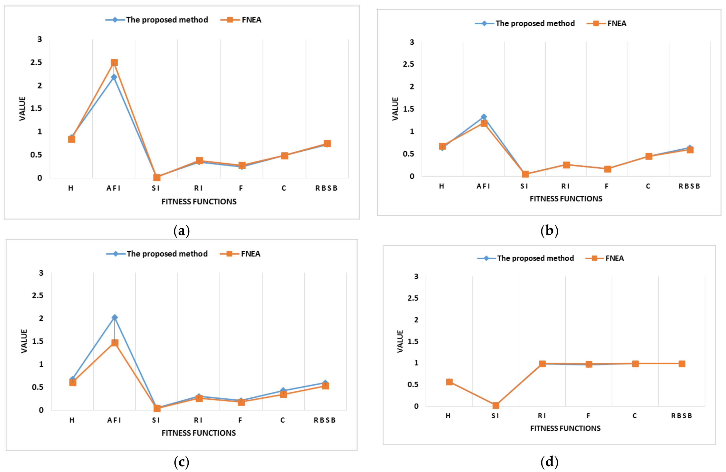
4.3.1. Accuracy Evaluation
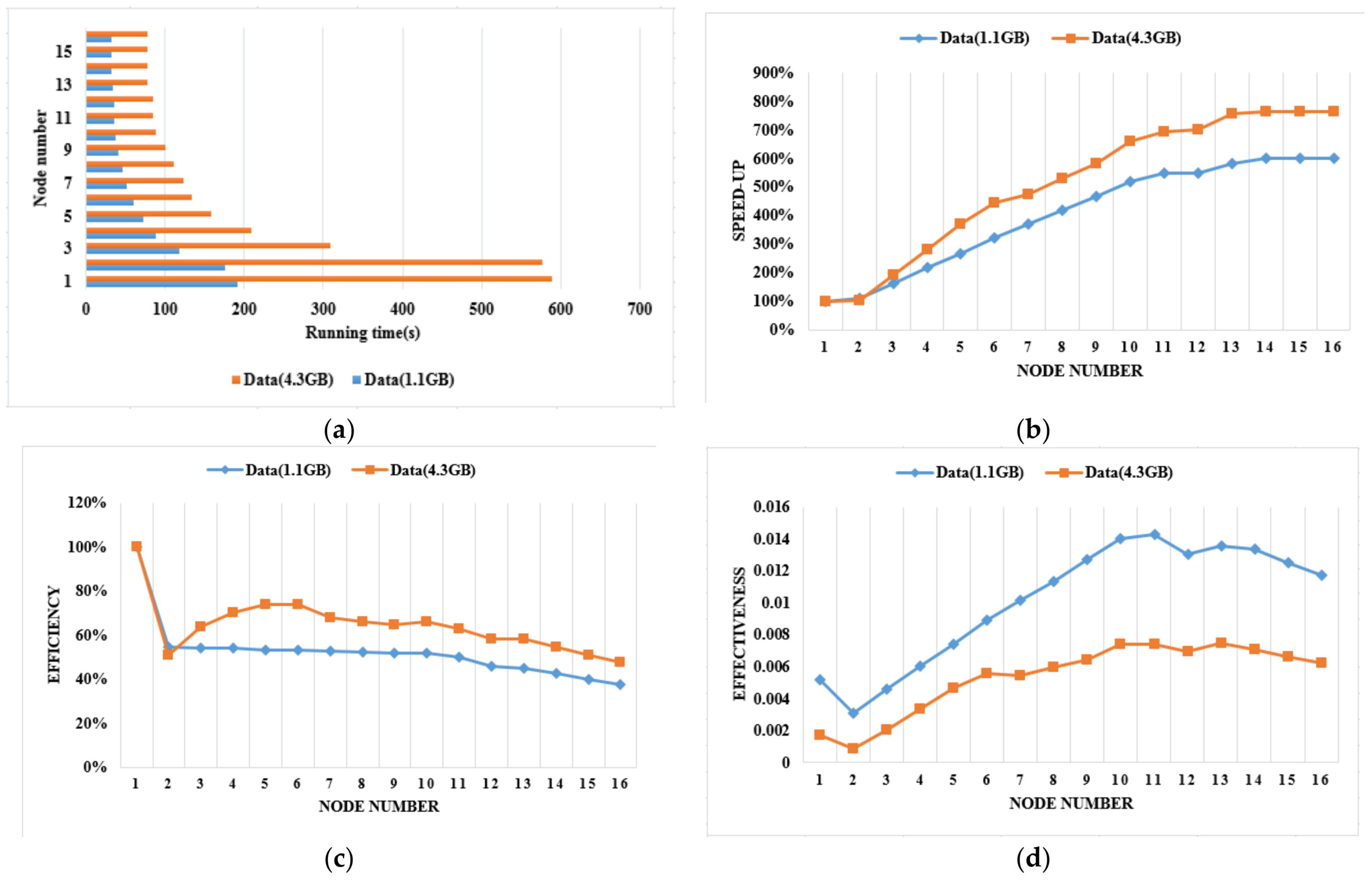
4.3.2. Speed Evaluation
5. Conclusions
Acknowledgments
Author Contributions
Conflicts of Interest
References
- Blaschke, T. Object based image analysis for remote sensing. ISPRS J. Photogramm. Remote Sens. 2010, 65, 2–16. [Google Scholar] [CrossRef]
- Blaschke, T.; Hay, G.J.; Kelly, M.; Lang, S.; Hofmann, P.; Addink, E.; Feitosa, R.; van der Meer, F.; van der Werff, H.; Van Coillie, F.; et al. Geographic Object-based Image Analysis: A new paradigm in Remote Sensing and Geographic Information Science. ISPRS J. Photogramm. Remote Sens. 2014, 87, 180–191. [Google Scholar] [CrossRef] [PubMed]
- Yuan, J.Y.; Wang, D.L.; Li, R.X. Remote Sensing Image Segmentation by Combining Spectral and Texture Features. IEEE Trans. Geosci. Remote Sens. 2014, 52, 16–24. [Google Scholar] [CrossRef]
- Wang, J.; Tang, J.L.; Liu, J.B; Ren, C.Y.; Liu, X.N.; Feng, J. Alternative Fuzzy Cluster Segmentation of Remote Sensing Images Based on Adaptive Genetic Algorithm. Chin. Geogr. Sci. 2009, 19, 83–88. [Google Scholar] [CrossRef]
- Judah, A.; Hu, B.X.; Wang, J.G. An Algorithm for Boundary Adjustment toward Multi-Scale Adaptive Segmentation of Remotely Sensed Imagery. Remote Sens. 2014, 6, 3583–3610. [Google Scholar] [CrossRef]
- Karantzalos, K.; Argialas, D. A Region-based Level Set Segmentation for Automatic Detection of Man-made Objects from Aerial and Satellite Images. Photogramm. Eng. Remote Sens. 2009, 75, 667–677. [Google Scholar] [CrossRef]
- Gaetano, R.; Masi, G.; Poggi, G. Marker-Controlled Watershed-Based Segmentation of Multiresolution Remote Sensing Images. IEEE Trans. Geosci. Remote Sens. 2015, 53, 2987–3004. [Google Scholar] [CrossRef]
- Michel, J.; Youssefi, D.; Grizonnet, M. Stable Mean-Shift Algorithm and Its Application to the Segmentation of Arbitrarily Large Remote Sensing Images. IEEE Trans. Geosci. Remote Sens. 2015, 53, 952–964. [Google Scholar] [CrossRef]
- Marpu, P.R.; Neubert, M.; Herold, H.; Niemeyer, I. Enhanced evaluation of image segmentation results. J. Spat. Sci. 2010, 55, 55–68. [Google Scholar] [CrossRef]
- Baatz, M.; Schäpe, A. Multiresolution segmentaion: An optimization approach for high quality multi-scale image segmentation. In Angewandte Geographische Informationsverarbeitung XII; Strobl, J., Blaschke, T., Griesebner, G., Eds.; Wichmann: Heidelberg, Germany, 2000; pp. 12–23. [Google Scholar]
- Deng, F.L.; Yang, C.J.; Cao, C.X.; Fan, X.Y. An Improved Method of FNEA for High Resolution Remote Sensing Image Segmentation. J. Geo-Inf. Sci. 2014, 16, 95–101. [Google Scholar]
- Peng, B.; Zhang, L.; Zhang, D. A Survey of Graph Theoretical Approaches to Image Segmentation. Pattern Recognit. 2013, 46, 1020–1038. [Google Scholar] [CrossRef]
- Beaulieu, J.M.; Goldberg, M. Hierarchy in Picture Segmentation: A Stepwise Optimization Approach. IEEE Trans. Pattern Anal. Mach. Intell. 1989, 11, 150–163. [Google Scholar] [CrossRef]
- Felzenszwalb, P.F.; Huttenlocher, D.P. Efficient Graph-Based Image Segmentation. Int. J. Comput. Vis. 2004, 59, 167–181. [Google Scholar] [CrossRef]
- Wang, S.; Siskind, J.M. Image Segmentation with Minimum Mean Cut. In Proceedings of the 8th IEEE International Conference on Computer Vision, Vancouver, BC, Canada, 7–14 July 2001; pp. 517–524. [Google Scholar]
- Wang, S.; Siskind, J.M. Image Segmentation with Ratio Cut. IEEE Trans. Pattern Anal. Mach. Intell. 2003, 25, 675–690. [Google Scholar] [CrossRef]
- Shi, J.B.; Malik, J. Normalised cuts and image segmentation. IEEE Trans. Pattern Anal. Mach. Intell. 2000, 22, 888–905. [Google Scholar]
- Dezső, B.; Giachetta, R.; László, I.; Fekete, I. Experimental study on graph-based image segmentation methods in the classification of satellite images. EARSeL eProc. 2012, 11, 12–24. [Google Scholar]
- Bue, B.D.; Thompson, D.R.; Gilmore, M.S.; Castano, R. Metric learning for hyperspectral image segmentation. In Proceedings of the 3rd IEEE WHISPERS, Lisbon, Portugal, 6–9 June 2011; pp. 1–4. [Google Scholar]
- Sırmaçek, B. Urban-Area and Building Detection Using SIFT Keypoints and Graph Theory. IEEE Trans. Geosci. Remote Sens. 2009, 47, 1156–1167. [Google Scholar] [CrossRef]
- Strîmbu, V.F.; Strîmbu, B.M. A graph-based segmentation algorithm for tree crown extraction using airborne LiDAR data. ISPRS J. Photogramm. Remote Sens. 2015, 104, 30–43. [Google Scholar] [CrossRef]
- Sharifi, M.; Kiani, K.; Kheirkhahan, M. A Graph-Based Image Segmentation Approach for Image Classification and Its Application on SAR Images. Prz. Elektrotech. 2013, 89, 202–205. [Google Scholar]
- Li, H.T.; Gu, H.Y.; Han, Y.S.; Yang, J.H. An efficient multi-scale SRMMHR (statistical region merging and minimum heterogeneity rule) segmentation method for high-resolution remote sensing imagery. IEEE J. Sel. Top. Appl. Earth Obs. Remote Sens. 2009, 2, 67–73. [Google Scholar] [CrossRef]
- Wang, M. A Multiresolution Remotely Sensed Image Segmentation Method Combining Rainfalling Watershed Algorithm and Fast Region Merging. Int. Arch. Photogramm. Remote Sens. Spat. Inf. Sci. 2008, 37, 1213–1218. [Google Scholar]
- Yang, Y.; Li, H.T.; Han, Y.S.; Gu, H.Y. High resolution remote sensing image segmentation based on graph theory and fractal net evolution approach. Int. Arch. Photogramm. Remote Sens. Spat. Inf. Sci. 2015, 40, 197–201. [Google Scholar] [CrossRef]
- Shen, Z.F.; Luo, J.C.; Chen, Q.X.; Sheng, H. High-efficiency Remotely Sensed Image Parallel Processing Method Study Based on MPI. J. Image Graph. 2007, 12, 133–136. [Google Scholar]
- Li, G.Q.; Liu, D.S. Key Technologies Research on Building a Cluster-based Parallel Computing System for Remote Sensing. In Proceedings of the 5th International Conference on Computational Science, Atlanta, GA, USA, 22–25 May 2005; Volume 3516, pp. 484–491. [Google Scholar]
- Schott, J.R. Remote Sensing: The Image Chain Approach; Oxford University Press: Oxford, UK, 2007; pp. 17–19. [Google Scholar]
- ISPRS Benchmarks. 2D Semantic Labeling Contest—Potsdam. Available online: http://www2.isprs.org/commissions/comm3/wg4/2d-sem-label-potsdam.html (accessed on 15 September 2016).
- Drǎguţ, L.; Tiede, D.; Levick, S.R. ESP: A tool to estimate scale parameter for multiresolution image segmentation of remotely sensed data. Int. J. Geogr. Inf. Sci. 2010, 24, 859–871. [Google Scholar] [CrossRef]
- Gao, Y.; Mas, J.F.; Kerle, N.; Navarrete Pacheco, J.A. Optimal region growing segmentation and its effect on classification accuracy. Int. J. Remote Sens. 2011, 32, 3747–3763. [Google Scholar] [CrossRef]
- Achanccaray, P.; Ayma, V.A.; Jimenez, L.I.; Bernabe, S.; Happ, P.N.; Costa, G.A.O.P.; Feitosa, R.Q.; Plaza, A. SPT 3.1: A free software tool for automatic tuning of segmentation parameters in optical, hyperspectral and SAR images. In Proceedings of the IEEE International Geoscience and Remote Sensing Symposium, Milan, Italy, 26–31 July 2015; pp. 4332–4335. [Google Scholar]
- Martha, T.R.; Kerle, N.; van Westen, C.J.; Jetten, V.; Kumar, K.V. Segment Optimization and Data-Driven Thresholding for Knowledge-Based Landslide Detection by Object-Based Image Analysis. IEEE Trans. Geosci. Remote Sens. 2011, 49, 4928–4943. [Google Scholar] [CrossRef]
- Stumpf, A.; Kerle, N. Object-oriented mapping of landslides using Random Forests. Remote Sens. Environ. 2011, 115, 2564–2577. [Google Scholar] [CrossRef]
- Myint, S.W.; Gober, P.; Brazel, A.; Grossman-Clarke, S.; Weng, Q. Per-pixel vs. object-based classification of urban land-cover extraction using high spatial resolution imagery. Remote Sens. Environ. 2011, 115, 1145–1161. [Google Scholar] [CrossRef]
- Pu, R.L.; Landry, S.; Yu, Q. Object-based urban detailed land-cover classification with high spatial resolution IKONOS imagery. Int. J. Remote Sens. 2011, 32, 3285–3308. [Google Scholar] [CrossRef]
- Johnson, B.A. Mapping Urban Land Cover Using Multi-Scale and Spatial Autocorrelation Information in High Resolution Imagery. Ph.D. Thesis, Florida Atlantic University, Boca Raton, FL, USA, May 2012. [Google Scholar]
- Zhang, Y.J. A survey on evaluation methods for image segmentation. Pattern Recognit. 1996, 29, 1335–1346. [Google Scholar] [CrossRef]
- Belgiu, M.; Dragut, L. Comparing supervised and unsupervised multiresolution segmentation approaches for extracting buildings from very high resolution imagery. ISPRS J. Photogram. Remote Sens. 2014, 96, 67–75. [Google Scholar] [CrossRef] [PubMed]
- Hoover, A.; Jean-Baptiste, G.; Jiang, X.; Flynn, P.J.; Bunke, H.; Goldgof, D.; Bowyer, K.; Eggert, D.W.; Fitzgibbon, A.; Fisher, R.B. An Experimental Comparison of Range Image Segmentation Algorithms. IEEE Trans. Pattern Anal. Mach. Intell. 1996, 18, 673–689. [Google Scholar] [CrossRef]
- Lucieer, A. Uncertainties in Segmentation and Their Visualisation. Ph.D. Thesis, Utrecht University and International Institute for Geo-Information Science and Earth Observation (ITC), Utrecht, The Netherlands, 2004. [Google Scholar]
- Neubert, M.; Meinel, G. Evaluation of Segmentation programs for high resolution remote sensing applications. In Proceedings of the Joint ISPRS/EARSeL Workshop “High Resolution Mapping from Space 2003”, Hannover, Germany, 6–8 October 2003; p. 8. [Google Scholar]
- Rand, W. Objective criteria for the evaluation of clustering methods. J. Am. Stat. Assoc. 1971, 336, 846–850. [Google Scholar] [CrossRef]
- Pont-Tuset, J.; Marques, F. Measures and Meta-Measures for the Supervised Evaluation of Image Segmentation. In Proceedings of the IEEE Conference on Computer Vision and Pattern Recognition (CVPR), Portland, OR, USA, 23–28 June 2013; pp. 2131–2138. [Google Scholar]
- Feitosa, R.Q.; Costa, G.A.O.P.; Cazes, T.B.; Feijo, B. A genetic approach for the automatic adaptation of segmentation parameters. In Proceedings of the 1st International Conference on Object Based Image Analysis, Salzburg, Austria, 4–5 July 2006; p. 31. [Google Scholar]
- Ma, L.; Fu, T.Y.; Blaschke, T.; Li, M.C.; Tiede, D.; Zhou, Z.J.; Ma, X.X.; Chen, D.L. Evaluation of feature selection methods for object-based land cover mapping of UAV imagery by RF and SVM classifiers. ISPRS Int. J. Geo-Inf. 2017, 6, 51. [Google Scholar] [CrossRef]


| Test | Imagery | Spatial Resolution (in m) | Number of Bands | Landscape Characteristics | Location |
|---|---|---|---|---|---|
| T1 | Airborne true orthophoto | 0.05 | 4 | residential/industrial area | Potsdam in Germany |
| T2 | SPECIM AISA EAGLE II image | 0.78 | 10 | residential/industrial area | DaFeng, in the Yancheng sub-province of Jiangsu province, in China |
| T3 | WorldView-2 image | 0.5 | 8 | residential/agriculture area | Lintong, in the Xi’an sub-province of Shanxi province, in the northwest of China. |
| T4 | RADARSAT-2 image | 8 | HH, HV, VH, VV | Agriculture area | Genhe, in the Hulunbeier sub-province of Inner Mongolia province, in China |
| Segmentation Parameters | Airborne | SPECIM AISA EAGLE II | WorldView-2 | RADARSAT-2 |
|---|---|---|---|---|
| weight of color () | 0.9 | 0.9 | 0.9 | 0.9 |
| weight of smoothness () | 0.5 | 0.5 | 0.5 | 0.5 |
| scale parameter (Q) | 240 | 360 | 260 | 2000 |
| Metrics | Formula | Explanations |
|---|---|---|
| Hoover Index (H) | Measures the number of correct detection based on the percentage of overlap between segmentation and reference ground truth (GT) [40]. CD is the number of correct detections and represents the number of segments in the GT image. Range [0,1], “H = 0” stands for perfect segmentation. | |
| Area-Fit-Index (AFI) | Addresses over-/under-segmentation by analyzing the overlapping area between segmentation and reference GT [41]. where Ak is the area, in pixels, of a reference segment Ck in the GT image, and Al.i.k is the area, in pixels, of the segment in the segmentation outcome S, with the largest intersection with the reference segment Ck. NGT is the number of segments in the GT image. “AFI = 0” stands for perfect overlap. | |
| Shape Index (SI) | Addresses the shape conformity between segmentation and reference GT [42]. where NGT is the number of segments in the GT image, ρi and ρj are the perimeters of the segments Ci and Cj, and Ai and Aj are their respective areas. Range [0,1], “SI = 0” stands for perfect segmentation. | |
| Rand Index (RI) | Measures the ratio between pairs of pixels that were correctly classified and the total pairs of pixels [43]. Let I = {𝑝1,…,𝑝N} be the set of pixels of the original image and consider the set of all pairs of pixels = {(𝑝i,𝑝j) I × I|i < j}. Moreover, Ci, a segment in the segmentation S, and Cj, a segment in the GT image, are considered as partitions of the image I. Then, is divided into four different sets depending on where a pair (𝑝i,𝑝j) of pixels falls: 11: in the same segment both in Ci and Cj. 10: in the same segment in Ci but different in Cj. 01: in the same segment in Cj but different in Ci. 00: in different segments both Ci and Cj. Range [0,1], “RI = 0” stands for perfect segmentation. | |
| Precision-Recall (F) | , | Measures the trade-off between Precision and Recall considering segmentation as a classification process [44]. Given a segment from the segmentation outcome S and a segment from its GT, four different regions can easily be differentiated: True positives (tp): pixels that belong to both S and GT. False positives (fp): pixels that belong to S but not to GT. False negatives (fn): pixels that belong to GT but not to S. True negatives (tn): pixels that do not belong to S or GT. Range [0,1], “F = 0” stands for perfect segmentation. |
| Segmentation Covering (C) | Measures the number of pixels of the intersection of two segments [44]. where ΣNGT is the total number of pixels in the original image. The overlap between two segments, Ci in a segmentation S and Cj in its GT, is defined as Range [0,1], “C = 0” stands for perfect segmentation. | |
| Reference Bounded Segments Booster (RBSB) | Measures the ratio between the number of pixels outside the intersection of two segments with the area of the reference GT [45]. where t represents a segment from GT and NGT is the number of segments in the GT image. fn, fp, tp is the same as Precision-Recall (F). Range [0,1], “RBSB = 0” stands for perfect segmentation. |
| Ground Truth Data | Airborne | SPECIM AISA EAGLE II | WorldView-2 | RADARSAT-2 |
|---|---|---|---|---|
| Classes, numbers of polygons | buildings and individual trees, 104 | big buildings, 28 | fields, 28 | fields, 21 |
| Airborne | SPECIM AISA EAGLE II | WorldView-2 | RADARSAT-2 | |||||
|---|---|---|---|---|---|---|---|---|
| Metrics | The Proposed Method | FNEA | The Proposed Method | FNEA | The Proposed Method | FNEA | The Proposed Method | FNEA |
| Hoover Index (H) | 0.88 | 0.84 | 0.64 | 0.68 | 0.68 | 0.61 | 0.58 | 0.57 |
| Area-Fit-Index (AFI) | 2.18 | 2.5 | 1.33 | 1.19 | 2.03 | 1.48 | 122.46 | 310.56 |
| Shape Index (SI) | 0.03 | 0.02 | 0.05 | 0.05 | 0.05 | 0.04 | 0.03 | 0.03 |
| Rand Index (RI) | 0.35 | 0.38 | 0.26 | 0.26 | 0.3 | 0.26 | 0.98 | 0.99 |
| Precision-Recall (F) | 0.25 | 0.28 | 0.17 | 0.17 | 0.21 | 0.18 | 0.96 | 0.98 |
| Segmentation Covering (C) | 0.49 | 0.49 | 0.45 | 0.45 | 0.43 | 0.35 | 0.99 | 0.99 |
| Reference Bounded Segments Booster (RBSB) | 0.73 | 0.75 | 0.64 | 0.6 | 0.6 | 0.53 | 0.99 | 0.99 |
| Metrics | Formula | Remarks |
|---|---|---|
| Speed-up | is the processing time of single computing node. is the processing time of P computing node. | |
| Efficiency | is the speed-up of P computing node. | |
| Effectiveness | is the efficiency of P computing node. |
© 2018 by the authors. Licensee MDPI, Basel, Switzerland. This article is an open access article distributed under the terms and conditions of the Creative Commons Attribution (CC BY) license (http://creativecommons.org/licenses/by/4.0/).
Share and Cite
Gu, H.; Han, Y.; Yang, Y.; Li, H.; Liu, Z.; Soergel, U.; Blaschke, T.; Cui, S. An Efficient Parallel Multi-Scale Segmentation Method for Remote Sensing Imagery. Remote Sens. 2018, 10, 590. https://doi.org/10.3390/rs10040590
Gu H, Han Y, Yang Y, Li H, Liu Z, Soergel U, Blaschke T, Cui S. An Efficient Parallel Multi-Scale Segmentation Method for Remote Sensing Imagery. Remote Sensing. 2018; 10(4):590. https://doi.org/10.3390/rs10040590
Chicago/Turabian StyleGu, Haiyan, Yanshun Han, Yi Yang, Haitao Li, Zhengjun Liu, Uwe Soergel, Thomas Blaschke, and Shiyong Cui. 2018. "An Efficient Parallel Multi-Scale Segmentation Method for Remote Sensing Imagery" Remote Sensing 10, no. 4: 590. https://doi.org/10.3390/rs10040590
APA StyleGu, H., Han, Y., Yang, Y., Li, H., Liu, Z., Soergel, U., Blaschke, T., & Cui, S. (2018). An Efficient Parallel Multi-Scale Segmentation Method for Remote Sensing Imagery. Remote Sensing, 10(4), 590. https://doi.org/10.3390/rs10040590